Utilizing Temporal Information for Taxonomy Construction
Luu Anh Tuan∗1, Siu Cheung Hui†2, See Kiong Ng#3∗Institute for Infocomm Research, Singapore
†School of Computer Engineering, Nanyang Technological University, Singapore
#Institute of Data Science, National University of Singapore
Abstract
Taxonomies play an important role in many applications by organizing domain knowledge into a hierarchy of ‘is-a’ relations between terms. Previous work on automatic construc-tion of taxonomies from text documents ei-ther ignored temporal information or used fixed time periods to discretize the time se-ries of documents. In this paper, we pro-pose a time-aware method to automatically construct and effectively maintain a taxon-omy from a given series of documents pre-clustered for a domain of interest. The method extracts temporal information from the docu-ments and uses a timestamp contribution func-tion to score the temporal relevance of the evidence from source texts when identifying the taxonomic relations for constructing the taxonomy. Experimental results show that our proposed method outperforms the state-of-the-art methods by increasing F-measure up to 7%-20%. Furthermore, the proposed method can incrementally update the taxon-omy by adding fresh relations from new data and removing outdated relations using an in-formation decay function. It thus avoids re-building the whole taxonomy from scratch for every update and keeps the taxonomy effec-tively up-to-date in order to track the latest in-formation trends in the rapidly evolving do-main.
1 Introduction
The explosion in the amount of unstructured text data gives us the opportunity to explore knowledge in depth, but there are also challenges to recog-nize useful information for our interests. To pro-vide access to information effectively, it is impor-tant to organize unstructured data in a structured and meaningful manner. Taxonomies, which serve as backbones for structured knowledge, are
use-ful for many NLP applications such as question answering (Harabagiu et al., 2003) and document clustering (Fodeh et al., 2011). However, hand-crafted, well-structured taxonomies such as Word-Net (Miller, 1995), OpenCyc (Matuszek et al., 2006) and Freebase (Bollacker et al., 2008), which are pub-licly available, can be incomplete for new or special-ized domains. As it is time-consuming and cum-bersome to create a new one manually, methods for automatic domain-specific taxonomy construc-tion from text corpora are highly desirable.
Previous work on automatic construction of domain-specific taxonomies from text documents assumed that the data sets (that is, the document sets) and the underlying taxonomic relations are
static. However, the data sets for certain domains may evolve over time, as new documents are added while older documents are deleted or modified. As such, the taxonomic relations for these potentially fast-changing domains may not remain static but become dynamic over time as new domain terms emerge while some older ones disappear. For ex-ample, in World Health Organization reports about
disease outbreak, the term‘smallpox’ used to be a hyponym of‘dangerous disease’, but it has fallen off since 1980. On the other hand, since 2014 the term
‘Ebola’has become an emerging hyponym of ‘dan-gerous disease’. As another example, up until 1992, in a collection of US yearly reports of terrorism, the term‘Palestine Liberation Organization’used to be a hyponym of‘terrorist group’, but it is no longer true nowadays. ‘Palestine Liberation Organization’
should now be classified as a‘national organization’
of Palestine.
When temporal information in data sets is not captured, the resultant taxonomy may be incom-plete or outdated and misleading. This could be caused by the overwhelming evidence of older pat-terns/contexts compared to emerging, but relatively
551
small amount of, evidence of newer relations. For example, in the taxonomy of US yearly reports on terrorism, many previous methods could fail to rec-ognize the taxonomic relation between the two terms
‘ISIS’ and ‘terrorist group’due to relatively infre-quent mentions of‘ISIS’(which only appears in re-ports from 2014). Meanwhile,‘Palestine Liberation Organization’could still be classified as a hyponym of‘terrorist group’because of the relatively larger number of mentions in the documents from the ear-lier years.
In this paper, we propose a time-aware method for domain-specific taxonomy construction from a time series of text documents for a particular do-main. We incorporate temporal information into the process of identifying taxonomic relations by com-puting evidence scores for the data sources weighted by a timestamp contribution function (Efron and Golovchinsky, 2011; Li and Croft, 2003) to cap-ture the temporally-varying contributions of evi-dence from various documents at a particular point in time. We assume that newer evidence is more im-portant than older evidence. For example, the evi-dence that‘Palestine Liberation Organization’was a hyponym of‘terrorist group’ in 1990 is less im-portant now than the evidence that ‘ISIS’ is a hy-ponym of‘terrorist group’in 2014. In the proposed method, we incorporate the timestamp contribution function into the method of Tuan et al. (2014) to measure the weights of the evidence for both sta-tistical and linguistic methods. With such built-in time-awareness for taxonomy construction, we en-sure that the constructed taxonomies are up-to-date for the fast-changing domains found in newswire and social media, where users constantly search for updated relations and track information trends.
Most previous work requires re-running the tax-onomy construction process whenever there are new incoming data. Our proposed method enables in-cremental update of the constructed taxonomies to avoid costly reconstructions. We incorporate an information decay function (Smucker and Clarke, 2012) to manage outdated relations in the con-structed taxonomy. The decay function measures the extent that the relation is out-of-date over time, and we incorporate it into a time-aware graph-based al-gorithm for taxonomy update.
The contributions of our research are summarized as follows:
• We propose a time-aware method for taxon-omy construction that extracts and utilizes tem-poral information to measure evidence weights of taxonomic relationships. Our method con-structs an up-to-date taxonomy by adding new emerging relations and discarding obsolete and incorrect ones.
• We propose an incremental time-aware
graph-based algorithm to update an existing taxon-omy, instead of rebuilding a new taxonomy from scratch.
2 Related Work
Previous work on taxonomy construction can be roughly divided into two main approaches: statis-tical learning and linguistic pattern matching. Sta-tistical learning methods for taxonomy construc-tion include co-occurrence analysis (Lawrie and Croft, 2003), hierarchical Latent Dirichlet Alloca-tion (LDA) (Blei et al., 2004), clustering (Li et al., 2013), term embedding (Tuan et al., 2016), linguis-tic feature-based semanlinguis-tic distance learning (Yu et al., 2011), and co-occurrence subnetwork mining (Wang et al., 2013). Supervised statistical methods (Petinot et al., 2011) rely on hierarchical labels to learn the corresponding terms for each label. The labeled training data, however, are costly to obtain and may not always be available in practice. Un-supervised statistical methods (Pons-Porrata et al., 2007; Li et al., 2013; Wang et al., 2013) are based on the idea that terms that frequently co-occur may have taxonomic relationships. However, these meth-ods generally achieve low accuracy.
Input documents & Web data
Temporal information processing
Sentence timestamp
Domain term extraction
Taxonomic relation identification
Taxonomy induction
Existing taxonomy
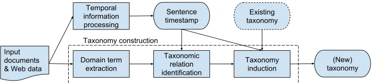
[image:3.612.116.498.46.132.2](New) taxonomy Taxonomy construction
Figure 1: Workflow of the proposed time-aware taxonomy construction method.
find taxonomic relations.
The approach that is closest to our work is the one proposed by Zhu et al. (2013), which performs dynamic taxonomy update. To keep up with ever changing social media data, new terms are mined from incoming data and added to the existing tax-onomy. The data are divided into separate clusters using pre-defined time periods based on their docu-ment timestamps. The newly found taxonomic re-lations in each period are then added to the exist-ing taxonomy. The use of a pre-defined time pe-riod to discretize the time series of the documents for taxonomy update can be problematic. If the cho-sen time period is too long, rapid changes of do-main terms and their taxonomic relations that have occurred within the time period may not be reported. If the time period is too short, it may fail to identify valid taxonomic relations that needed a longer time period to establish. The method also does not re-move those relations in the existing taxonomy that may have become obsolete over time.
3 Problem Specification
We define the root term of a domain-specific taxon-omy as a word or phrase that represents the domain of interest. It can be any informative concept such as an entity (‘animal’) or event (‘Ebola outbreak’). Given a root termR, we define a corpusCas a pre-clustered set of a time series of text documents ac-cording toR.
Given two terms t1 and t2, we denote t1 → t2
as a taxonomic relation wheret1 is a hypernym of
t2. In this work, we define a taxonomy as a triple H= (V, E, s), where:
• V is the set of the taxonomy’s vertices, i.e., the
set of terms, including the root term.
• E is the set of the taxonomy’s edges, i.e., the
set of taxonomic relations.
• sis the creation time of the taxonomy. It can
be the current date or any specified time.
Our task is formally defined as follows: Given a root term R, a corpus C and an optional existing taxonomyH1 = (V1, E1, s1)constructed at times1, we aim to build a new taxonomyH2 = (V2, E2, s2) at time s2, where s2 > s1, so that we can process the document set inCup to times2 into the relevant terms in the taxonomy.
If H1 does not exist, the problem becomes
cre-ating a taxonomyH2 for corpus C. Otherwise, the
problem is to update the existing taxonomy with the newly obtained data for corpusC. Note that while
the taxonomy construction method is not a totally unsupervised method as it does require as input a corpus (C) pre-clustered by a domain of interest (i.e., R), the subsequent steps for constructing the taxon-omy given the text corpus are unsupervised.
4 Methodology
Figure 1 shows the workflow of the proposed time-aware taxonomy construction method. There are two key processes in the proposed method: temporal information processing and taxonomy construction.
4.1 Temporal information processing
The aim of the temporal information processing pro-cess is to generate temporal information (or times-tamp for short) for each sentence in the input docu-ment or Web data.
Previous taxonomy construction methods (Zhu et al., 2013) only extract temporal information at the document level, i.e., all information in the document has the same timestamp as the document creation date. This assumption, however, is not always cor-rect. Figure 2 shows a sample report about the flight
Figure 2: A sample report about the flightMH370created on 30 July 2015.
method to extract timestamps (i.e., temporal expres-sions) at the sentence level. The method comprises the following three steps:
Document creation date extraction: First, we ex-tract the timestamp at the document level. The text corpus that we are using for this study consists of a collection of reports, scientific publications and Web search results. For the first two types of documents, the timestamp is the document creation date that can be extracted directly from the data source, i.e., the date of the report, or the date of the publication. For Web search results, we use Google advanced search with customized time range which returns the search results together with their creation dates at the begin-ning of search snippets.
Temporal expression extraction: Next, the sec-ond step proceeds to extract all temporal expressions (e.g. “2015 December 31”) in the document. Here, we use SUTime (Chang and Manning, 2012), a li-brary for recognizing and normalizing time expres-sion using a deterministic rule-based method. The output of this step is a list of time expressions, to-gether with their positions in the document.
Sentence timestamp extraction and normaliza-tion: Finally, in the third step, we assign each sen-tence in the document a time expression as follows:
• First, we assign a temporal valueτ as the
doc-ument creation date.
• For each sentencesin the document:
– Ifscontains a temporal expressionτ1, assign
τ1 as the timestamp ofsand updateτ =τ1.
– Otherwise, assignτ as the timestamp ofs. Note that we use the format ‘YYYY-MM-DD’ for the temporal expression. If the information of DD or MM is missing, it is replaced with the first day
or first month respectively. For example, ‘December 2015’ will be normalized as ‘2015-12-01’. Using the proposed method, sentence (1) and sentence (2) in the example of Figure 2 will have the same times-tamp of ‘2014-03-08’, while sentence (3) will have the timestamp of ‘2014-03-17’.
In Section 5.2, we will show that the extraction of timestamps at the sentence level will improve the performance of the proposed taxonomy construction method as compared to the extraction of timestamps at the document level.
4.2 Taxonomy construction
There are three general steps to constructing a tax-onomy: domain term extraction, taxonomic relation identification, and taxonomy induction. We make use of the taxonomy construction method of Tuan et al. (2014) for the first step, incorporate times-tamps into the second step of identifying taxonomic relations (Section 4.2.2), and propose an incremen-tal taxonomy induction algorithm for the third step (Section 4.2.4). As extraction of domain term ex-traction does not affect the temporal aspects of tax-onomy construction, the first step of domain term extraction is not within the scope of this study. The reader can refer to Tuan et al. (2014) or Zhu et al. (2013) in which linguistic approaches to extract do-main terms are discussed. In this paper, we assume that the list of domain terms is available and we will focus only on discussing the second and third steps for taxonomy construction.
4.2.1 Taxonomic relation identification
In this section, we give an overview of the method to identify taxonomic relations proposed in Tuan et al. (2014). Given an ordered pair of two termst1and
t2, Tuan et al. (2014) calculates the evidence score
thatt1 →t2based on the following three methods:
Syntactic contextual subsumption (SCS): This
method derives evidence fort1 →t2from their
syn-tactic contexts, particularly from triples of the form (subject, verb, object). It is observed that if the context set oft1 mostly contains that oft2 but not
vice versa, thent1 is likely to be a hypernym oft2.
To implement this idea, the method finds the most common relation (orverb)roft1andt2, submits the
queries “t1 r” and “t2 r” to Web search engine and
CorpusΓt1 andCorpusΓt2 fort1 andt2. The
syntac-tic context sets are then created from these contex-tual corpora using a non-taxonomic relation identifi-cation method. The details ofScoreSCS(t1, t2)can
be found in Tuan et al. (2014).
Lexical-syntactic pattern (LSP):This method is to find how much more evidence fort1 → t2is found
on the Web than fort2 → t1. Specifically, a list of
manually constructed taxonomic patterns (e.g., “t2
is at1”) is queried with a Web search engine to
es-timate the amount of evidence fort1 → t2 from the
Web. The LSP measure is calculated as follows:
ScoreLSP(t1, t2) =
log(|CW eb(t1, t2)|) 1 +log(|CW eb(t2, t1)|) whereCW eb(t1, t2)denotes the set of search results.
String inclusion with WordNet (SIWN): This
method is to check the evidence fort1 →t2by using
the combination of string inclusion and references in WordNet synsets. ScoreSIW N(t1, t2) is set to 1 if
there is such evidence; otherwise, it is set to 0.
Combined evidence: The three scores are then
combined linearly as follows:
Score(t1, t2) = α×ScoreSCS(t1, t2) +β×ScoreLSP(t1, t2) +γ×ScoreSIW N(t1, t2)
IfScore(t1, t2)is greater than a threshold value,
thent1is regarded as a hypernym oft2.
4.2.2 Incorporating temporal information into taxonomic relation identification
Previous studies of taxonomic relation identifi-cation treated all evidence equally, i.e., evidence from 1950 is treated equally with evidence from 2014. This assumption is not always appropriate, as discussed in Section 1. We propose a time-aware method to identify taxonomic relations by incorpo-rating timestamps into the process of finding evi-dence, using the following timestamp contribution function:
Definition 1 (Timestamp contribution function).
Given a text sentencedwith timestampsd, the
times-tamp contribution ofdat times0is defined as:
Td(s0) =ξe−ξ(s0−sd), (1)
whereξ is a control rate,s0 > sdand(s0−sd)is the time lapse betweensdands0.
Equation (1) describes the timestamp contribution of a sentence at a specific time by using an expo-nential distribution function Td. The intuition
be-hind this function is that the evidence of taxonomic relations found in more recent sentences will be of higher relevance than that found in older sentences. This function is inspired by the work of Efron and Golovchinsky (2011), and Li and Croft (2003), in which it was used to effectively rank documents over time intervals.
Using the timestamp contribution function, we in-corporate temporal information into the three taxo-nomic relation identification methods described in Section 4.2.1, as follows:
LSP method: For each search result snippet din CW eb(t1, t2)collected from the Web search engine,
we calculate the timestamp contribution score of d
by using Td: Td(s0) = ξe−ξ(s0−sd), where s0 is a
chosen specific time (i.e., the time of taxonomy con-struction) and sd is the timestamp of d. Note that
sd has to be earlier thans0. The unit of time lapse
(s0−sd)depends on the nature of corpus and can be,
for instance, a day, a month or even a year. For ex-ample, if the corpus is from a fast-changing source such as social media, we can set the unit as day to keep up with the change of data on a daily basis. In contrast, for a corpus from slower changing domains such as scientific disciplines, the unit can be a year. The time-aware score for the LSP method is calcu-lated as follows:
ScoreT imeLSP (t1, t2) =ScoreLSP(t1, t2)
×
P
d∈CW eb(t1,t2)Td(s0)
|CW eb(t1, t2)|
(2)
In Equation (2), the original LSP evidence score is multiplied by the average timestamp contribution score of all evidence sentences for the taxonomic re-lation from the Web. If the number of the returned search results is too large, we will use only the first 1,000 results to estimate the average timestamp con-tribution of evidence.
Note that the total timestamp contribution score of all evidence sentencesPd∈CW eb(t1,t2)Td(s0)can be
considered as the “weighted size” ofCW eb(t1, t2),
i.e., we weigh each evidence sentence using Equa-tion (1) and sum all these weights. However, if we use only the “weighted size” ofCW eb(t1, t2)for the
time-aware score ScoreT imeLSP (t1, t2), there will be
some issues. Firstly, the score ScoreT ime
be normalized with respect to the number of evi-dence sentences. This may lead to potential bias due to large amounts of past evidence—if there were an obsolete or incorrect taxonomic relation with many evidence sentences in the past, it may overwhelm the new taxonomic relations which may only have a small number of recent evidence sentences. Sec-ondly, if we normalize the score, the information on the number of evidence sentences, which is im-portant for theLSP method to recognize true
taxo-nomic relationships, will be lost. Therefore, we pro-pose to use Equation (2), which combines both in-formation on the number of evidence sentences (em-bedded inside the originalScoreLSP score) and the
normalized “weighted size” ofCW eb(t1, t2).
SCS method:Similarly, for each search result snip-petdinCorpusΓt1 andCorpusΓt2, we calculate the
timestamp contribution score ofdusing the function Td: Td(s0) = ξe−ξ(s0−sd), where s0 is a specific
time andsd is the timestamp ofd. The time-aware
score for SCS method is calculated as follows:
ScoreT imeSCS(t1, t2) =ScoreSCS(t1, t2)
×
P
d1∈CorpusΓ t1
Td1(s0) |CorpusΓ
t1|
+ P
d2∈CorpusΓ t2
Td2(s0) |CorpusΓ
t2|
(3) In Equation (3), the original evidence score of
t1→t2is multiplied by the average timestamp
con-tribution scores of the returned search snippets. Sim-ilar to Equation (2), Equation (3) combines both in-formation on the number of evidence sentences (em-bedded inside the original scoreScoreSCS) and the
normalized “weighted size” of them.
SIWN method:Because WordNet does not contain information about timestamps, we set:
ScoreT imeSIW N(t1, t2) =ScoreSIW N(t1, t2) (4)
Combined evidence: The final combined evidence score for the time-aware method is calculated as:
ScoreT ime(t1, t2) = α×ScoreT imeSCS(t1, t2) +β×ScoreT imeLSP (t1, t2) +γ×ScoreT imeSIW N(t1, t2)
(5)
If the value ScoreT ime(t1, t2) is greater than a
threshold value, we extract the relationt1→t2.
4.2.3 Parameter learning
We need to estimate the optimal values for the pa-rametersα,βandγ which are used in Equation (5).
For this purpose, we apply ridge regression (Hastie et al., 2009). First, we use the time-aware method to create taxonomies for the ‘Animal’, ‘Plant’ and ‘Ve-hicle’ domains using corpora constructed by a boot-strapping method (Kozareva et al., 2008). Then, we ask two annotators to construct gold standard tax-onomies of the three domains (see Section 5.2 for more details) and use them to build the training sets. For each pair of terms (t1, t2) found in the gold
stan-dard taxonomies, its evidence score is estimated as (τ+1), whereτis the threshold value forScoreT ime.
Finally, we use Equation (5) to learn the best combi-nation ofα,βandγusing the ridge regression
algo-rithm. Note that we learn the parameters only once and use them subsequently for the other domains.
4.2.4 Incremental taxonomy induction
To avoid reconstructing a taxonomy whenever there is new incoming data, we propose a novel in-cremental graph-based algorithm to update an exist-ing taxonomy with a given set of taxonomic rela-tions. The proposed algorithm updates a taxonomy automatically over time based on the information decay function defined below.
Definition 2 (Information decay function). Given a taxonomic relationr, the information decay ofr
over the period from times1 to times2 is computed by the information decay function:
Dr(s1, s2) =e−λ(s2−s1), (6) whereλis a decay rate ands2 > s1.
The intuition behind the information decay func-tion is that the evidential value of a relafunc-tion will de-crease over time at an exponential rate.
Given a root node R, a set of taxonomic
rela-tionsT and, optionally, an existing taxonomyH1=
(V1, E1, s1)created at times1with vertex setV1and
edge set E1, the proposed graph-based algorithm
constructs a new taxonomyH2 = (V2, E2, s2)
cre-ated at times2 with vertex setV2 and edge setE2.
t1 → t2 denotes the edge from t1 tot2 in a
taxon-omy, andw(t1 →t2)as the weight of this edge (i.e.,
evidence score). Algorithm 1 consists of four steps:
Algorithm 1Taxonomy induction algorithm
Input: R: root node of taxonomy; T: new taxonomic relation set;
H1= (V1, E1, s1): existing taxonomy created at time
s1with vertex setV1and edge setE1;
Output: H2= (V2, E2, s2): new taxonomy created at time
s2with vertex setV2and edge setE2; 1: SetV2=V1andE2=E1
2: foreach edge (t1→t2)∈E2,t16=Randt26=Rdo 3: w(t1→t2) =w(t1→t2)×e−λ(s2−s1) 4: end for
5: foreach relation (t1→t2)∈T do 6: if(t1→t2)∈E2then
7: w(t1→t2)=w(t1→t2) +ScoreT ime(t1, t2) 8: else
9: E2=E2∪(t1→t2)
10: w(t1→t2)=ScoreT ime(t1, t2) 11: ift16∈V2then
12: V2=V2∪ {t1}
13: end if
14: ift26∈V2then 15: V2=V2∪ {t2}
16: end if
17: if@(t3→t1)∈E2andt36=Rthen 18: E2=E2∪(R →t1)
19: w(R →t1)= 1
20: end if
21: if∃(R →t2)∈Ethen 22: E2=E2\(R →t2)
23: end if
24: end if
25: end for
26: edgeFiltering(H2); 27: graphPruning(H2);
times1 tos2. In this step, the weight of each edge
(t1 → t2) inE1(except the edges connected to root R) is reduced using the information decay function:
w(t1 →t2) =w(t1 →t2)×Dt1→t2(s1, s2)
Step 2: Add new relations to existing taxonomy
(lines 5 - 25) This step adds new taxonomic relations to the existing taxonomy and updates their weights. It adds each relationt1 →t2as a directed edge from
the parent nodet1 to child nodet2 if this edge does
not exist in the existing taxonomy. Otherwise, we update the weight of this edge with a new evidence score. Ift1 does not have any parent node, t1 will
become a child node of rootR. The edge’s weight is updated as follows:
w(t1 →t2) =
1 ift1=R
w(t1→t2) +ScoreT ime(t1, t2)
ift1→t2∈E1
ScoreT ime(t
1, t2) otherwise
The result of this step is a weighted connected graph containing all taxonomic relations with rootR.
Step 3: Edge filtering (line 26) The graph gener-ated in Step 2 contains some edges with low evi-dence scores. The reason is that some relations in the existing taxonomy can become outdated during the period froms1 tos2 (according to the
informa-tion decay funcinforma-tion), and they do not exist in the new relation set. In this step, each edget1 → t2 in the
graph is revisited, and if its weight is lower than the threshold value of ScoreT ime, it will be removed
from the graph. In the case thatt2 does not have
any other parent node except t1,t2 will be deleted
from the vertex set, and edges from t1 tot2’s
chil-dren will be added to the edge set with weights that are equal to the weights of the edges fromt2tot2’s
children. Then, all edges from t2 to t2’s children
will be removed from the edge set.
Step 4: Graph pruning(line 27) The graph gener-ated in Step 3 is not an optimal tree as it may con-tain redundant edges or incorrect edges—for exam-ple, those edges that form a loop in the graph. This step aims to produce an optimal tree of the taxon-omy from the weighted graph in Step 3. For this purpose, we apply Edmonds’ algorithm (Edmonds, 1967) for finding the optimal spanning arborescence for a weighted directed graph. Using this algorithm, we can find a subset of the current edge set that forms a taxonomy where every non-root node has in-degree 1 and the sum of the edge weights is max-imized.
5 Performance Evaluation
We have conducted two experiments for perfor-mance evaluation. The first experiment evaluates the performance of our proposed time-aware method on constructing a taxonomy from a given list of terms without any prior knowledge (i.e., without any exist-ing taxonomies). The second experiment evaluates the performance of our proposed method on taxon-omy update.
5.1 Datasets
We evaluate our method for taxonomy construction based on the following four datasets of document collections obtained from different domains:
• Artificial Intelligence (AI) domain (Navigli et
from 1969 to 2014 and the ACL archives from year 1979 to 2014.
• MH370 domain: The corpus is about the root
term ‘Issues related to MH370 search’. MH370 is the missing flight that went down in the ocean on Saturday, 8 March 2014. The corpus is created by querying the Google search en-gine with the keyword “MH370” from March 08, 2014 to April 30, 2014 and collecting the first 300 documents from the search results each day. After removing duplicates, the cor-pus contains a total of 12,307 documents.
• Terrorism domain: The corpus is about the root
term ‘Terrorism’. It contains 293 reports from “Patterns of Global Terrorism (1988-2003)”
1 and “Country Reports on Terrorism
(2004-2014)”2 of the US state department. Each
re-port contains about 1,500 words.
• Disease domain: The corpus is about the root term ‘Disease outbreak’, created by collecting reports from “Disease outbreaks by year from 1996 to 2014”3of WHO, and the email archive
of ProMed4which is an email based reporting
system dedicated to reporting on disease out-breaks that affect human health. The corpus contains a total of 25,370 reports/emails.
Parameter settings. For the rapidly changing do-main ‘MH370’, we choose ‘day’ as the unit of the time lapse whereas for the other three domains, we use ‘year’ as the time lapse unit. We set the thresh-old value ofScoreT imein Equation (5) as 2.2, and
the control rateξin Equation (1) and decay rateλin
Equation (6) as 0.15. The setting of these parameters will be discussed in Section 5.4.
5.2 Evaluation on taxonomy construction 5.2.1 Experiment
In this experiment, we compare our time-aware taxonomy construction method with other state-of-the-art methods in the task of constructing a new taxonomy from a given list of terms without any prior knowledge (i.e., without any existing taxon-omy). Three state-of-the-art methods in the litera-ture are selected for comparison:
1http://www.fas.org/irp/threat/terror.htm 2http://www.state.gov/j/ct/rls/crt/index.htm 3http://www.who.int/csr/don/archive/year/en/ 4http://www.promedmail.org/
• Zhu’s method (Zhu et al., 2013): It constructs the taxonomy using evidence from multiple sources such as WordNet, Wikipedia and Web search engines. In their method, both statisti-cal and linguistic approaches are used to infer taxonomic relations.
• Kozareva’s method (Kozareva and Hovy,
2010): It constructs the taxonomy using evi-dence from a Web search engine by matching the search results with a predefined set of syn-tactic patterns.
• Tuan’s method (Tuan et al., 2014): It is the non
time-aware method described in Section 4.2.1. This method ignores temporal information dur-ing taxonomy construction.
To evaluate the effectiveness of extracting times-tamps at the sentence level (as described in Section 4.1), we also conduct an experiment on a setting that uses the timestamps out the document level (i.e., all evidence in the document will have the same times-tamp information as the document creation date). We use the subscriptdocstampto denote this setting.
5.2.2 Evaluation metric
In this experiment, we evaluate the constructed taxonomies against the manually created gold stan-dard taxonomies. The gold stanstan-dard taxonomies are created as follows. For each domain, two annotators are employed at the same time to create taxonomies independently using the list of terms obtained from the domain term extraction module, according to the following rules:
• Rule 1 (Relevancy): Every term in the
taxon-omy should be related to the root term.
• Rule 2 (Appropriateness): Each edge between
two terms should be established at the time the taxonomy is created, if their relation is correct and not obsolete. A relation is obsolete if it is invalid at the time of consideration.
• Rule 3 (Hierarchical structure): The gold
stan-dard taxonomy of each domain should form a tree, without redundant paths or cycles. The annotators then compare their constructed taxonomies. A taxonomic relation t1 → t2 is
counted as an agreement if and only if both an-notators have t1 and t2 in their taxonomies, and
there is a directed path from t1 to t2. If an
Domain Number of vertices Average depth
MH370 257 3.2
AI 925 5.3
Terrorism 312 3.6
[image:9.612.314.541.46.290.2]Disease 459 4.0
Table 1: Analysis of gold standard taxonomies.
in the other annotator’s taxonomy, it will be consid-ered as a disagreement. After evaluation, the aver-age inter-annotator agreement on edges of the con-structed taxonomies between the two annotators is 87% using Cohen’s kappa coefficient measurement. Finally, the two annotators discuss to come up with the gold standard taxonomies. As a result, the num-ber of nodes and average depth of the taxonomies are summarized in Table 1. We use precision, re-call and F-measure to measure the performance of taxonomy construction. LetRandRgold be the set
of taxonomic relations of our constructed taxonomy and the gold standard taxonomy respectively; then the metrics are given as follows:
precision= |R∩Rgold|
|R| ; recall=
|R∩Rgold| |Rgold|
;
F-measure= 2×precision×recall
precision+recall.
5.2.3 Experimental results
The experimental results are given in Table 2 which shows that our time-aware method achieves significantly better performance than Kozareva’s method and Zhu’s method in terms of F-measure (t-test, p-value<0.05). Our method shows slightly
lower precision than that of Kozareva’s method due to the SCS method, but much higher recall and F-measure than Kozareva’s method. In contrast, our method shows slightly lower recall but much higher precision and F-measure than Zhu’s method, which is based on statistical methods such as pointwise mutual information and cosine similarity. On aver-age, our time-aware method improves the F-measure by 20% compared to Kozareva’s method, and by 10% compared to Zhu’s method.
Moreover, the incorporation of timestamps into the time-aware method also contributes to better per-formance as it helps identify new taxonomic rela-tions effectively, while getting rid of obsolete and incorrect relations. As shown from the experimental results, the time-aware method shows significantly better performance than the non time-aware method (i.e. Tuan’s method) in all four domains in terms of
Method Domain P R F
Kozareva MH370 89% 36% 51%
Zhu MH370 60% 59% 59%
Tuan MH370 85% 49% 62%
Time-awaredocstamp MH370 81% 54% 65%
Time-aware MH370 86% 57% 69%
Kozareva AI 90% 37% 52%
Zhu AI 59% 57% 58%
Tuan AI 84% 51% 63%
Time-awaredocstamp AI 80% 55% 65%
Time-aware AI 84% 57% 68%
Kozareva Terrorism 91% 32% 47%
Zhu Terrorism 60% 64% 62%
Tuan Terrorism 86% 49% 62%
Time-awaredocstamp Terrorism 80% 56% 66%
Time-aware Terrorism 87% 60% 71%
Kozareva Disease 90% 29% 44%
Zhu Disease 57% 56% 56%
Tuan Disease 83% 50% 62%
Time-awaredocstamp Disease 81% 53% 64%
Time-aware Disease 85% 55% 67%
Table 2: Experimental results for taxonomy construction. P stands for Precision, R for Recall, and F for F-measure.
F-measure (t-test, p-value<0.05). On average, our time-aware method improves the F-measure by 7% compared to Tuan’s method.
We further examine the taxonomic relations iden-tified by the time-aware method but not by the non-time-aware method, and vice versa. We observed that around 91% of relations found by the time-aware method but not by the non-time-time-aware method are recent relations (i.e., relations found in recent documents), while around 86% of relations found by the non-aware method but not by the time-aware method are obsolete relations. The percentage of taxonomic relations that become obsolete in each of the datasets are summarized in Table 3.
Domain Percentage of obsolete relations
MH370 21%
AI 5%
Terrorism 12%
[image:9.612.88.281.52.109.2]Disease 7%
Table 3: Percentage of taxonomic relations that become obsolete.
[image:9.612.336.518.538.596.2]and ‘terrorist group’, our method was able to ig-nore it. The reason is that the three state-of-the-art methods inferred taxonomic relations using co-occurrence frequency, but‘ISIS’ has only appeared in reports since 2014. The occurrence frequency of
‘ISIS’ was very low compared to ‘Palestine Liber-ation OrganizLiber-ation’which was mentioned over the past many years. In contrast, by using the timestamp contribution function to better profile the relevance of evidence over time, our method can recognize the recent relationship of ‘terrorist group’ with ‘ISIS’
while getting rid of the obsolete and incorrect rela-tion with‘Palestine Liberation Organization’.
From the experimental results of the time-aware and time-awaredocstamp methods, we also observe
that the use of timestamps extracted at the sentence level is more effective than the use of timestamps at the document level. The timestamps extracted at the sentence level can capture more precisely the tempo-ral information of the facts in fast-changing domains than those at the document level. The results showed that the use of sentence-level timestamps can im-prove the precision and recall of our taxonomy con-struction method, improving the F-measure by 4% on average, as compared to the use of timestamps at the document level.
5.3 Evaluation on taxonomy update 5.3.1 Experiment
For fast-changing domains, taxonomies should be frequently and quickly updated. In this experiment, we examine how the proposed time-aware method can effectively update the constructed taxonomies over time to keep up with the latest information trends.
We use the case study of the ‘MH370’ domain for this experiment. During the search operation for the missing flight MH370, there were several turning points which can be captured by the follow-ing phases (accordfollow-ing to well-known news agencies such as CNN, BBC and the New York Times):
• Phase 1 (from March 08, 2014): The flight lost contact with the airport. The search started from the South China Sea and Gulf of Thailand, and was extended to the Strait of Malacca.
• Phase 2 (from March 13, 2014): Images from satellites indicated the plane might have fallen into the Indian Ocean. The search focus was
moved from the South of Sumatra to the South-West of Perth in the Southern Indian Ocean.
• Phase 3 (from March 28, 2014): Estimation of
the aircraft’s remaining fuel and the radar track led the search to shift to a new area, the North-West of Perth in the Southern Indian Ocean. We apply the proposed time-aware method to con-struct and update the taxonomy for ‘MH370’ incre-mentally every two days. We compare our time-aware method with the following three methods:
• Zhu’s method (Zhu et al., 2013): It applies a graph-based algorithm to update taxonomies incrementally with timestamp information.
• Baseline 1: The taxonomy is updated with the
newly obtained data every two days, but does not use any temporal information in either tax-onomic relation identification (Section 4.2.2) or taxonomy induction (Section 4.2.4). Specifi-cally, Step 1 (update existing taxonomy) in Sec-tion 4.2.4 is excluded since we are not using any temporal information, so there is no updat-ing of the weights of the existupdat-ing taxonomy us-ing the decay function.
• Baseline 2: We construct the taxonomies using
temporal information every two days, but only with the new documents from these two days. This allows us to evaluate the effect of retiring all the taxonomic relations built from the pre-vious documents instead of the gradual decay approach in our proposed method.
Here we have chosen the time period of two days because the ‘MH370’ domain was a truly fast-changing domain. As we shall see shortly, even us-ing only the new documents within 2 days to build the taxonomy in our baseline method 2, there were new taxonomic relations updated from the latest in-formation (as shown in the example in Figure 4).
5.3.2 Evaluation metric
When constructing the gold standard taxonomies using the same rules described in Section 5.2, we asked the annotators to select for each parent term at most three sub-terms that are most related to it at the time of taxonomy construction. We denote the set of gold-standard taxonomic relations asSgold. In
at most three sub-terms with the highest evidence scores. We denote the set of those automatically ex-tracted taxonomic relations asS. We use the
follow-ing metrics to evaluate the update of taxonomy:
precision=|S∩Sgold|
|S| ; recall=
|S∩Sgold| |Sgold|
;
F-measure= 2×precision×recall
precision+recall.
The intuition for limiting the sub-term number to three for the evaluation is that if a taxonomy can keep up with the newly updated data, it should be able to detect the emerging terms and relations and add them to the taxonomy with high evidence scores so that the user can easily observe an emerging trend of information in the domain as it occurs. In addi-tion, the method should also have the capability to remove any obsolete relations in the taxonomy when they are no longer valid.
5.3.3 Experimental results
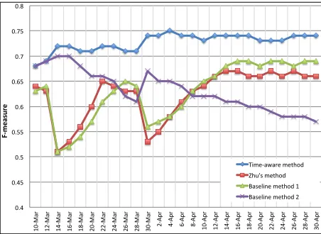
From the results shown in Figure 3, we can see that our time-aware method achieves the best performance and significantly outperforms the two baseline methods and Zhu’s method in terms of F-measure (t-test, p-value<0.05). One
interest-ing point to observe is that there are two periods when the time-aware method shows much higher F-measure than the baseline methods and Zhu’s method: from March 12 to March 14, and from March 28 to March 30. During these periods, the performance of baseline method 1 (which does not use any timestamp information) and Zhu’s method drops significantly, while our time-aware method’s performance increases slightly.
One plausible explanation is that there are some turning points on March 13 and March 28, which fall within these periods as described above. Dur-ing these periods, many new terms/relations such as search area, search focus and search device are added to the corpus. Our time-aware method was able to assign higher weights to the new taxonomic relations than the older relations due to their recent timestamps, even though the frequencies of these new relations are fewer than that of the older re-lations. In contrast, Zhu’s method and baseline method 1 were unable to recognize these new rela-tions due to their relatively low frequencies in the corpus. In addition, incorrect relations in the exist-ing taxonomy were also removed from the new
[image:11.612.314.540.48.213.2]tax-0.4$ 0.45$ 0.5$ 0.55$ 0.6$ 0.65$ 0.7$ 0.75$ 0.8$ 10 *Mar $ 12 *Mar $ 14 *Mar $ 16 *Mar $ 18 *Mar $ 20 *Mar $ 22 *Mar $ 24 *Mar $ 26 *Mar $ 28 *Mar $ 30 *Mar $ 2*Ap r$ 4*Ap r$ 6*Ap r$ 8*Ap r$ 10*Ap r$ 12*Ap r$ 14*Ap r$ 16*Ap r$ 18*Ap r$ 20*Ap r$ 22*Ap r$ 24*Ap r$ 26*Ap r$ 28*Ap r$ 30*Ap r$ F" m ea su re )
Figure 3: Performance results on taxonomy update over time in the ‘MH370’ domain.
onomy using the information decay function by our time-aware method, whereas the other two methods still kept them in the taxonomy. In short, our time-aware method can update the taxonomy faster with the latest information trends, as well as remove in-correct relations effectively, as compared to the other methods.
[image:11.612.83.288.109.158.2]Also, from the experimental results of our time-aware method and the baseline method 2, we can observe that updating the existing taxonomy with new taxonomic relations is more effective than re-building a new taxonomy using only the new data. The reason is that although some older taxonomic relations are mentioned occasionally in the new data, they are still valid. Therefore, if we ignore the older data, their taxonomic relations will be lost in the new taxonomy when it is constructed with only the new data. In addition, there are also many taxonomic re-lations that needed a longer time period to become established.
South China Sea
Gulf of Thailand
Malacca Strait Zhu’s
method
Baseline method 1
Time-aware method
2014-03-12 2014-03-14 2014-03-26 2014-03-30 2014-04-30 South China Sea
Gulf of Thailand
Southern Indian Ocean
Southern Indian Ocean
South China Sea
Sumatra
South China Sea
Gulf of Thailand
Malacca Strait
South China Sea
Southern Indian Ocean
Gulf of Thailand
Southern Indian Ocean
South China Sea
Sumatra
South China Sea
Malacca Strait
Gulf of Thailand
Southern Indian Ocean
Sumatra
South China Sea
Southern Indian Ocean
South-West of Perth
South China Sea
Southern Indian Ocean
South China Sea
South-West of Perth
North-West of Perth
Southern Indian Ocean
South-West of Perth
North-West of Perth
Southern Indian Ocean
South China Sea
North-West of Perth
Southern Indian Ocean
South China Sea
North-West of Perth
Southern Indian Ocean
2014-03-13 2014-03-28
Actual search area: South China Sea, Malacca Strait, Gulf of Thailand
Actual search area: Sumatra, South-West of Perth, Southern Indian Ocean
Actual search area: North-West of Perth, Southern Indian Ocean
Baseline method 2
South China Sea
Malacca Strait
Gulf of Thailand
Southern Indian Ocean
Sumatra
South China Sea
Southern Indian Ocean
South-West of Perth
North-West of Perth
Southern Indian Ocean
North-West of Perth
Southern Indian Ocean
Southern Indian Ocean
Sumatra
[image:12.612.81.530.45.310.2]South-West of Perth
Figure 4: Top three hyponyms of ‘Search area’ in ‘Issues related to MH370 search’ taxonomies over time.
and baseline method 1 both missed this update un-til March 26. Another interesting point is that due to the lack of temporal information, both Zhu’s method and baseline method 1 still ranked‘South China Sea’
at the top of the taxonomies constructed on April 30, while this term was removed earlier from the hyponym list of ‘search area’ by our time-aware method using temporal information.
5.4 Parameter tuning
In our method for taxonomy construction, some pa-rameters are tuned to optimize performance.
The threshold value for ScoreT ime in Equation
(5) controls the number of extracted taxonomic re-lations. In general, the larger this threshold value is, the higher number of true taxonomic relations we can get. However, a higher number of incorrect re-lations may also occur. From our experiments, we found that the threshold value forScoreT imecan be
set between 2.1 to 2.3 for the time-aware method to achieve the best performance.
The control rateξin Equation (1) and decay rate λin Equation (6) affect the contribution of old and
new data. Specifically, smaller values for the trol rate and decay rate will allow newer data to con-tribute more evidence of taxonomic relations than older data, whereas larger values will cause the old and new data to have similar evidence
contribu-tions. According to our experiments, the time-aware method shows the best performance when the values of these rates are set between 0.15 to 0.20.
6 Conclusion
In this paper, we have proposed a novel time-aware method for taxonomy construction given a time se-ries of text documents from a domain that could be fast-changing with emerging concepts or events. By using timestamp contribution and information decay functions, our method can effectively utilize tempo-ral information for both taxonomic relation identifi-cation and taxonomy update. The experimental re-sults show that our method achieves better perfor-mance than the state-of-the-art methods. In addi-tion, the proposed method can be used to update the taxonomy incrementally over time and keep the tax-onomy up-to-date with the latest information trends for the domain. All the datasets, including the gold standards of the four domains and the outputs of our method, are publicly available at https://sites. google.com/site/tuanluu219/research/tacl1.
Acknowledgements
References
David M. Blei, Thomas L. Griffiths, Michael I. Jordan, and Joshua B. Tenenbaum. 2004. Hierarchical Topic Models and the Nested Chinese Restaurant Process.
Advances in Neural Information Processing Systems, pages 17–24.
Kurt Bollacker, Colin Evans, Praveen Paritosh, Tim Sturge, and Jamie Taylor. 2008. Freebase: A Col-laboratively Created Graph Database for Structuring Human Knowledge. Proceedings of the ACM SIG-MOD International Conference on Management of Data, pages 1247–1250.
Angel X. Chang and Christopher D. Manning. 2012. SUTIME: A Library for Recognizing and Normaliz-ing Time Expressions. Proceedings of the Conference on Language Resources and Evaluation, pages 3735– 3740.
Jack Edmonds. 1967. Optimum Branchings. Journal of Research of the National Bureau of Standards B, 71:233–240.
Miles Efron and Gene Golovchinsky. 2011. Estimation Methods for Ranking Recent Information. Proceed-ings of the 34th ACM SIGIR conference, pages 495– 504.
Samah Fodeh, Bill Punch, and Pang N. Tan. 2011. On Ontology-driven Document Clustering Using Core Se-mantic Features. Knowledge and Information Sys-tems, 28(2):395–421.
Sanda M. Harabagiu, Steven J. Maiorano, and Marius A. Pasca. 2003. Open-domain Textual Question An-swering Techniques. Natural Language Engineering, 9(3):231–267.
Trevor Hastie, Robert Tibshirani, and Jerome H. Fried-man. 2009. The Elements of Statistical Learning. Springer-Verlag.
Marti A. Hearst. 1992. Automatic Acquisition of Hy-ponyms from Large Text Corpora. Proceedings of the 14th Conference on Computational Linguistics, pages 539–545.
Zornitsa Kozareva and Eduard Hovy. 2010. A
Semi-supervised Method to Learn and Construct Tax-onomies Using the Web. Proceedings of the Confer-ence on Empirical Methods in Natural Language Pro-cessing, pages 1110–1118.
Zornitsa Kozareva, Ellen Riloff, and Eduard H. Hovy. 2008. Semantic Class Learning from the Web with Hyponym Pattern Linkage Graphs.Proceedings of the 46th Annual Meeting of the ACL, pages 1048–1056. Dawn J. Lawrie and W. Bruce Croft. 2003. Generating
Hierarchical Summaries for Web Searches. Proceed-ings of the 26th ACM SIGIR conference, pages 457– 463.
Xiaoyan Li and Bruce W. Croft. 2003. Time-based Lan-guage Models. Proceedings of the 12th ACM CIKM conference, pages 469–475.
Baichuan Li, Jing Liu, Chin-Yew Lin, Irwin King, and Michael R. Lyu. 2013. A Hierarchical Entity-based Approach to Structuralize User Generated Content in Social Media: A Case of Yahoo! Answers. Proceed-ings of the EMNLP conference, pages 1521–1532. Cynthia Matuszek, John Cabral, Michael J. Witbrock,
and John DeOliveira. 2006. An Introduction to the Syntax and Content of CYC.Proceedings of the AAAI Spring Symposium, pages 44–49.
George A. Miller. 1995. WordNet: A Lexical Database for English.Communications of the ACM, 38(11):39– 41.
Roberto Navigli, Paola Velardi, and Stefano Faralli. 2011. A Graph-based Algorithm for Inducing Lexical Taxonomies from Scratch. Proceedings of the 20th In-ternational Joint Conference on Artificial Intelligence, pages 1872–1877.
Yves Petinot, Kathleen McKeown, and Kapil Thadani. 2011. A Hierarchical Model of Web Summaries. Pro-ceedings of the 49th Annual Meeting of the ACL, pages 670–675.
Aurora Pons-Porrata, Rafael Berlanga-Llavori, and Jose Ruiz-Shulcloper. 2007. Topic Discovery Based on Text Mining Techniques. Information processing & management, 43(3):752–768.
Mark D. Smucker and Charles L. Clarke. 2012. Time-based Calibration of Effectiveness Measures. Pro-ceedings of the 35th ACM SIGIR conference, pages 95–104.
Luu A. Tuan, Jung J. Kim, and See K. Ng. 2014. Tax-onomy Construction using Syntactic Contextual Evi-dence. Proceedings of the EMNLP conference, pages 810–819.
Luu A. Tuan, Yi Tay, Siu C. Hui, and See K. Ng. 2016. Learning Term Embeddings for Taxonomic Relation Identification Using Dynamic Weighting Neural Net-work. Proceedings of the EMNLP conference, pages 403–413.
Chi Wang, Marina Danilevsky, Nihit Desai, Yinan Zhang, Phuong Nguyen, Thrivikrama Taula, and Jiawei Han. 2013. A Phrase Mining Framework for Recursive Construction of a Topical Hierarchy. Proceedings of the 19th ACM SIGKDD conference, pages 437–445. Wentao Wu, Hongsong Li, Haixun Wang, and Kenny Q.
Zhu. 2012. Probase: A Probabilistic Taxonomy for Text Understanding. Proceedings of the ACM SIG-MOD conference, pages 481–492.
Jianxing Yu, Zheng-Jun Zha, Meng Wang, Kai Wang, and Tat-Seng Chua. 2011. Domain-assisted Product As-pect Hierarchy Generation: Towards Hierarchical Or-ganization of Unstructured Consumer Reviews. Pro-ceedings of the EMNLP conference, pages 140–150. Xingwei Zhu, Zhao Y. Ming, and Tat-Seng Chua. 2013.