New special cases of the quadratic assignment problem with diagonally structured coefficient matrices

Original citation:

Cela, E., Deineko, Vladimir G. and Worginger, G.. (2018) New special cases of the quadratic assignment problem with diagonally structured coefficient matrices. European Journal of Operational Research, 267 (3). pp. 818-834.

Permanent WRAP URL:

http://wrap.warwick.ac.uk/96371

Copyright and reuse:

The Warwick Research Archive Portal (WRAP) makes this work by researchers of the University of Warwick available open access under the following conditions. Copyright © and all moral rights to the version of the paper presented here belong to the individual author(s) and/or other copyright owners. To the extent reasonable and practicable the material made available in WRAP has been checked for eligibility before being made available.

Copies of full items can be used for personal research or study, educational, or not-for-profit purposes without prior permission or charge. Provided that the authors, title and full bibliographic details are credited, a hyperlink and/or URL is given for the original metadata page and the content is not changed in any way.

Publisher’s statement:

© 2018, Elsevier. Licensed under the Creative Commons Attribution-NonCommercial-NoDerivatives 4.0 International http://creativecommons.org/licenses/by-nc-nd/4.0/

A note on versions:

The version presented here may differ from the published version or, version of record, if you wish to cite this item you are advised to consult the publisher’s version. Please see the ‘permanent WRAP url’ above for details on accessing the published version and note that access may require a subscription.

New special cases of the Quadratic Assignment

Problem with diagonally structured coefficient

matrices

Eranda C¸ ela∗ Vladimir Deineko† Gerhard J. Woeginger‡

Abstract

We consider new polynomially solvable cases of the well-known Quadratic Assignment Problem involving coefficient matrices with a special diagonal structure. By combining the new special cases with polynomially solvable special cases known in the literature we obtain a new and larger class of polynomially solvable special cases of the QAP where one of the two coefficient matrices involved is a Robinson matrix with an additional structural property: this matrix can be represented as a conic combination of cut matrices in a certain normal form. The other matrix is a conic combination of a monotone anti-Monge matrix and a down-benevolent Toeplitz matrix. We consider the recognition problem for the special class of Robinson matrices mentioned above and show that it can be solved in polynomial time.

Keywords. combinatorial optimization; quadratic assignment; Robinsonian; cut matrix; Monge matrix; Kalmanson matrix.

1

Introduction

In this paper we investigate the Quadratic Assignment Problem (QAP), which is a well-known problem in combinatorial optimization; we refer the reader to the book [9] by C¸ ela and the book [6] by Burkard, Dell’Amico & Martello for comprehensive surveys on the QAP. The QAP in Koopmans-Beckmann form [25] takes as input two n×n square matrices A = (aij)

and B = (bij) with real entries and will be denoted by QAP(A, B). The goal is to find a

permutation π that minimizes the objective function

Zπ(A, B) := n

X

i=1

n

X

j=1

aπ(i)π(j)bij. (1)

Equivalently the objective function can be written as hAπ, Bi = T r(AπBT), where Aπ = (aπ_ij) = (a_π(i)π(j)) is the matrix which results from matrixA after permuting both its rows and

∗

[email protected]. Institut f¨ur Diskrete Mathematik, TU Graz, Steyrergasse 30, A-8010 Graz, Austria, Corresponding author

†

[email protected]. Warwick Business School, Coventry, CV4 7AL, United Kingdom

‡

its columns according to permutation π. T r is the trace operator andT r(AπBT) is the trace of the product of the matricesAπ andB. The formulation of the goal function of the QAP by means of the trace operator is used in many applications, see eg. [9, 19]. Hereπ ranges over the set Sn of all permutations of{1,2, . . . , n}.

The QAP is a notoriously difficult problem both from the practical and from the theoretical point of view. In spite of the amazing development of computer and software technology nowadays it is still considered a challenge to exactly solve moderate size instances of size more than 30, i.e. n ≥ 30 [30]. From the theoretical point of view Sahni and Gonzalez [40] have shown that no constant-factor approximation algorithm exists for the QAP unless P =N P. Queyranne [36] has shown that the existence of a constant-factor approximation algorithm for

QAP(A, B) impliesP =N P even in the case whereAis the distance matrix of a set of points in the Euclidean line andB is a block-diagonal symmetric 0-1-matrix with zeroes on the main diagonal.

One branch of research on the QAP concentrates on the algorithmic behavior of strongly structured special cases; see for instance Burkard & al [5], Deineko & Woeginger [18], C¸ ela & al [13], C¸ ela, Deineko & Woeginger [10], and Laurent and Seminaroti [27] for typical results in this direction.

In our paper we follow recent developments and present several new results in this exciting area of research. In particular we discuss two new polynomially solvable special cases (p.s.s. cases) of the QAP involving diagonally structured matrices, see Definition 2.2. The new p.s.s. cases arethe down-benevolent QAP and the up-benevolent QAP. The down-benevolent QAP is a QAP(A, B) with A being both a Kalmanson and a Robinson matrix (see Definition 2.6 and 2.1, respectively) and B being a down-benevolent Toeplitz matrix (see Definition 2.2). This problem is solved to optimality by the identity permutation which will be denoted byid

in the sequel. This new p.s.s. case is related to two other p.s.s. cases of the QAP known in the literature: (a)QAP(A, B) with Abeing a Kalmanson matrix andB being a DW Toeplitz matrix (see [18] and Definition 2.6), and (b)QAP(A, B) withAbeing a Robinson matrix and

B being a simple Toeplitz matrix [27]. In the new p.s.s. case matrix A is more special and matrix B is more general than in the previous two p.s.s. cases. The up-benevolent QAP is a QAP(A,B) with A being a PS anti-Monge matrix (see Definition 3.7) and B being an up-benevolent Toeplitz matrix (see Definition 2.2). This problem is solved to optimality by the identity permutation. This new p.s.s. case is a generalization of another p.s.s. case of the QAP known in the literature, namely QAP(A, B) where A is a symmetric monotone anti-Monge matrix andB is an up-benevolent Toeplitz matrix [5].

Further we focus on the so-called combined p.s.s. cases of the problem. They arise as a combination of different p.s.s. cases of the QAP which involve matrices of the same type1. This approach is interesting because it allows the identification of new and more complex p.s.s. cases of the QAP. In particular we show that aQAP(A, B) with Abeing a conic combination of a symmetric anti-Monge matrix (see Definition 2.6) and a down-benevolent Toeplitz matrix (see Definition 2.2) andB being a conic combination of cut matrices in CDW normal form (see Definition 2.4) is solved by the identity permutation. Further we tackle a relevant question in this context, namely the recognition of cut matrices in CDW normal form, and show that it

1

can be decided efficiently.

Motivation. A direct, intrinsic and purely theoretical motivation is the identification of further p.s.s. cases and the better delimitation of the border between “simple” and “hard” cases of the QAP. From a more practical point of view, while being indeed very special and highly structured some of the p.s.s. cases discussed in this paper appear when modeling the

seriation problem, which in turn has practical applications, for example in archaeology, gene sequencing, or order recovering for disordered Markov chains, see Fogel et al. [19] and the references therein.

Moreover it would be interesting to investigate whether the combined special cases of the QAP can be used to compute good lower bounds and/or heuristic solutions for the general problem. The idea is to “approximate” the coefficient matrices A and B of a given instance

QAP(A, B) by some matrices A0 and B0, respectively, such that QAP(A0, B0) is an instance of a combined p.s.s. special case. Then, if A0 and B0 are chosen “appropriately”, the optimal solution ofQAP(A0, B0) and its optimal value could serve as a heuristic solution and/or a lower bound forQAP(A, B), respectively. Clearly, the crucial part is to find out what “approximate” and “appropriately” should mean, and this is definitely a challenging issue.

Outline of the paper. The paper is organized as follows. In Section 2 we define the matrix classes which play a role in the p.s.s. cases discussed in this paper and review relevant results from the literature. In the Section 3 we introduce two new p.s.s. cases of the QAP, the so-called down-benevolent QAP in Section 3.1, and the up-benevolent QAP in Section 3.2. Then in Section 3.3 we extend the variety of known p.s.s. cases of the QAP by introducing the so-called combined p.s.s. cases. Section 4 deals with conic representations of specially structured matrices. In Section 4.1 Kalmanson matrices and matrices which are both Kalmanson and Robinson matrices are characterized in terms of conic combinations of particular cut matrices. These results are then used in Section 4.2 to give a characterization of conic combinations of cut-matrices in CDW normal form. This characterization allows the efficient recognition of conic combinations of cut matrices in CDW normal form. Notice that this recognition problem is relevant because the conic combinations of cut matrices in CDW normal form are involved in the first combined p.s.s. case described in Section 3.3. We conclude with a summary of results and some issues for further research in Section 5.

2

Preliminaries and definitions

There are already quite a number of results known on p.s.s. cases of the QAP where the coefficient matricesA and B possess specific structural properties. We provide an overview of this kind of p.s.s. cases by introducing a classification of the involved coefficient matrices with particular properties and distinguish the following matrix classes.

Matrices with monotonicity properties including Robinson dissimilarities (called Robin-son matrices in the following), RobinRobin-son similarities, monotone matrices, see Defini-tion 2.1 later in this secDefini-tion.

and down-benevolent Toeplitz matrices, see Definition 2.2.

Matrices with block structural properties including block matrices, cut matrices and cut matrices in CDW normal form, see Definition 2.4.

Matrices defined in terms of four-point conditions including Monge matrices, anti-Monge matrices and Kalmanson matrices, see Definition 2.6.

Sum matrices and constant matrices including sum matrices, weak sum matrices and weak constant matrices, see Definition 2.8.

Further we recall some existing results on p.s.s. cases where these matrix classes are involved.

Definition 2.1 (Matrices with monotonicity properties)

A symmetric matrixA= (aij) is a Robinson dissimilarity or briefly a Robinson matrix, if for alli < j < k it satisfies the conditions aik≥max{aij, ajk}; in words, the entries in the matrix are placed in non-decreasing order in each row and column when moving away from the main diagonal.

A symmetric matrix A= (aij) is a Robinson similarity, if for all i < j < k it satisfies the conditions aik≤min{aij, ajk}. 2

An n×n matrix B = (bij) is called monotone, if bij ≤bi,j+1 and bij ≤bi+1,j holds for all

i, j∈ {1,2, . . . , n}, that is, if the entries in every row and column are sorted non-decreasingly from the left to the right and from the top to the bottom, respectively.

In some QAP special cases considered in this paper the diagonal elements of the coefficient matrices do not impact the optimal solution. In these cases we assume them to be zero and setaii= 0, for alli.

The Robinson matrices were first introduced by Robinson [38] in 1951 in the context of an analysis of archaeological data. Since then they have been widely used in combinatorial data analysis; see the books [21, 22, 31, 32] and the surveys [3, 8] for examples of various applications of Robinson structures in quantitative psychology, analysis of DNA sequences, cluster analysis, etc. Special cases of the QAP involving Robinson matrices are discussed in Laurent and Seminaroti [27] and in Fogel et al. [19].

Definition 2.2 (Matrices with diagonal structural properties)

Ann×nmatrixB = (bij) is called a Toeplitz matrixif it has constant entries along each of its diagonals; in other words, there exists a functionf:{−n+1,−n+2, . . . ,−1,0,1, . . . , n−1} →R such that bij =f(i−j), for all 1≤i, j≤n. The Toeplitz matrix B is fully determined by the functionf and therefore f will be calledthe generating function ofB. Iff(i) =f(i−n) holds for everyi∈ {1,2, . . . , n−1}, the Toeplitz matrix B is called a circulant matrix.

A symmetric Toeplitz matrix whose generating function f fulfills f(0) = 0 and f(1) ≥

f(2)≥. . . ≥f(n−1) will be called a simple Toeplitz matrix. (Notice that a simple Toeplitz

2

matrix is a Toeplitz Robinson similarity with zeroes on the main diagonal.) These matrices were introduced by Laurent and Seminaroti [27].

A symmetric n×n circulant matrix B whose generating function f fulfills f(0) = 0,

f(1) ≥f(2) ≥. . . ≥ f(dn−₂1e) is called a DW-Toeplitz matrix. (Notice that in a symmetric circulant matrix f(i) =f(n−i) holds for all i >dn−1

2 e). These matrices were introduced in

Deineko and Woeginger [18].

A symmetric n×nToeplitz matrix B whose generating functionf fulfillsf(0) = 0, f(1)≤

f(2) ≤ . . . ≤ f(dn−1

2 e) and f(i) ≤ f(n−i), for all i ≤ d

n−1

2 e, is called an up-benevolent Toeplitz matrix. These matrices where introduced in [5] as benevolent Toeplitz matrices.

Analogously a symmetricn×nToeplitz matrixBwhose generating functionf fulfillsf(0) = 0, f(1) ≥ f(2) ≥ . . . ≥ f(dn−1

2 e) and f(i) ≥ f(n−i), for all i ≤ d

n−1

2 e, is called a down-benevolent Toeplitz matrix.

Finally the attributes down-benevolent and up-benevolent will be also used for the generating functions of the Toeplitz matrices having the corresponding properties, respectively. So we will talk about down-benevolent functions and up-benevolent functions defined over {−n+ 1, . . . ,−1,0,1, . . . , n−1}.

The structures introduced above appeared in several special cases of the QAP dealt with in the papers already cited in Introduction. One of the most recent results was presented by Laurent & Seminaroti in [27], and will be of special interest in the context of the paper at hand.

Theorem 2.3 (Laurent & Seminaroti [27])

QAP(A, B), where A is a Robinson matrix and B is a simple Toeplitz matrix is solved to optimality by the identity permutation.

To help readers to better understand structures involved in various QAP special cases, we use here a color coding to visualize these structures. Figure 1 illustrates Robinson matrices and simple Toeplitz matrices - the darker the color the larger the value of the corresponding matrix entries; the white color corresponds to zero entries. The instances of matrices used for the illustrations can be found in Appendix.

Definition 2.4 (Matrices with block structural properties)

Let a q×q matrixP = (pij) be fixed. An n×nmatrixB = (bij) is called a block matrix with

block patternP if the following holds

(i) there exists a partition of the set of row and column indices {1, . . . , n} into q (possibly empty) setsI1, . . . , Iq such that for 1≤k≤q−1 all elements of Ik are smaller than all elements ofIk+1,

(ii) for all pairs of indices (i, j) with i∈ Ik and j ∈ I` the equality bij =pk` holds, for all

k, `∈ {1,2, . . . , q}

A B

Figure 1: Illustration of the QAP instance considered in Laurent & Seminaroti QAP[27]: A -Robinson dissimilarity, B - simple Toeplitz matrix; the darker the color the larger the entries of the matrix.

Acut matrixB is a block matrix whose block pattern has0’s along the main diagonal and1’s everywhere else. A cut matrix is in CDW normal form, if its block sizes are in non-decreasing order, i.e. |I1| ≤ |I2| ≤ · · · ≤ |Iq|holds. (These matrices were introduced in [11].)

It is easy to see that any cut matrix is a Robinson matrix. Theorem 2.3 implies that if

A is a cut matrix and B is a simple Toeplitz matrix, then the QAP is solved by the identity permutation. Another p.s.s. case of the QAP involving cut matrices which will be of special interest in the context of this paper was identified by C¸ ela, Deineko & Woeginger [11].

Theorem 2.5 (C¸ ela, Deineko & Woeginger [11])

QAP(A, B), where A is a cut matrix in CDW normal form and B is a monotone anti-Monge matrix (see Definition 2.6) is solved to optimality by the identity permutation.

As a consequence of this result QAP(A, B) where A is a Robinson matrix obtained as a conic combination of cut matrices in CDW normal form, (i.e., A is a linear combination of such matrices with non-negative weight coefficients) andB is a monotone anti-Monge matrix is solved by the identity permutation. This special case is illustrated in Figure 2. The fulfillment of the anti-Monge inequalities is illustrated by the symbol “+”. Notice that the block structure of matrix A is not that obvious any more in the picture.

In the context of the special case mentioned in Theorem 2.5 the recognition of Robinson matrices, which can be represented as conic combinations of cut matrices in CDW normal form, becomes relevant:

Given an n×n Robinson matrix, can it be represented as a conic combination of cut matrices in CDW normal form?

A B

Figure 2: Illustration of a generalisation of the Cela, Deineko & Woeginger QAP [11]: A - a conic combination of Block matrices in CDW normal form, B - anti-Monge monotone matrix; the darker the color the larger the entries of the matrix.

classK or not. Recognition problems can be highly non-trivial. There are a number of papers dealing with recognition problems for different (permuted) classes of matrices, especially also for Robinson matrices [1, 15, 26, 28].

As an illustrative example for the recognition of a conic combination of cut matrices in CDW normal form we consider the following Robinson matrix:

C=



      

0 1 2 3 3 3

1 0 2 3 3 3

2 2 0 2 3 3

3 3 2 0 2 2

3 3 3 2 0 1

3 3 3 2 1 0



      

which is obtained as a sum of three cut-matricesC=C1+C2+C3; here matrixC1 has the three blocks {1,2,3}, {4}, {5,6}, matrix C2 has three blocks {1,2}, {3}, {4,5,6}, and matrix C3 has five blocks{1},{2},{3,4},{5}, and {6}. As none of these matrices above is a cut matrix in CDW normal form, there are no reasons to assume that the QAP withC and a monotone anti-Monge matrixB is solved by the identity permutation. In Section 4.2 we will revisit this example after the proof of Theorem 4.6 and will show that C can indeed be represented as a conic combination of cut matrices in CDW normal form. Hence the corresponding QAP is solved by the identity permutation.

Definition 2.6 (Matrices defined in terms of four point conditions)

An n×n matrix B is a Monge matrix, if its entries are non-negative and satisfy the Monge inequalities

In other words, in every2×2 submatrix the sum of the entries on the main diagonal is smaller than the sum of the entries on the other diagonal. (The Monge property essentially dates back to the work of Gaspard Monge [33] in the 18th century.)

Analogously, an n×n matrix B is an anti-Monge matrix, if its entries are non-negative and satisfy the anti-Monge inequalities

bij+brs ≥ bis+brj for 1≤i < r≤n and 1≤j < s≤n. (3)

A symmetric n×nmatrix(cij) is called a Kalmanson matrix, if it satisfies the conditions

cij+ckl≤cik+cjl (4)

cik+cjl≥cil+cjk (5)

for all i,j,k and l with 1 ≤i < j < k < l ≤n. (These matrices were introduced in 1975 by Kenneth Kalmanson [23].)

Kalmanson matrices can be also defined as matrices which fulfill the following inequalities:

ci,j+1+ci+1,j≤cij+ci+1,j+1 ∀i, j : 1≤i≤n−3, i+ 2≤j≤n−1, (6)

ci,1+ci+1,n ≤cin+ci+1,1 ∀i: 2≤i≤n−2. (7)

In this equivalent characterisation (proved for example in [16, 17]), the fulfillment of (4)-(5) is required just forO(n2) quadruples of entries.

Much research has been done on the role played by these classes of matrices in combinatorial optimization, in particular with respect to p.s.s. cases of hard combinatorial optimization problems arising when (one of) the input matrices belongs to some of those classes. Probably the first reference in this context is due to Supnik [41], while the term “four point conditions” was independently introduced by Quintas & Supnick [37] and Buneman [4].

Monge structures play a special role in p.s.s. cases of the QAP [5, 11, 13]. We refer the reader to the survey [7] by Burkard, Klinz & Rudolf for more general information on Monge and anti-Monge structures.

Kalmanson matrices play a role in p.s.s. cases of the QAP [18] and also in special cases of a number of other combinatorial optimization problems as the travelling salesman problem [23], the prize-collecting TSP [14], the master tour problem [17], the Steiner tree problem [24], the three-dimensional matching problem [35].

A special case of the QAP involving a Kalmanson matrix and relevant also in the context of this paper was considered by Deineko & Woeginger [18].

Theorem 2.7 (Deineko & Woeginger [18])

The QAP(A,B) where A is a Kalmanson matrix and B is a DW-Toeplitz matrix is solved to optimality by the identity permutation.

This special case is illustrated in Figure 3. The inequalities (4) and (5) fulfilled by the entries of the Kalmanson matrix C are illustrated by the “+” and “-”, respectively.

A B

Figure 3: Illustration of the Deineko & Woeginger QAP[18] : A - a Kalmanson matrix, B - a DW-Toeplitz matrix.

Definition 2.8 (Sum matrices and constant matrices)

An n×nmatrix A= (aij) is called a sum matrix, iff there exist real numbers α1, . . . , αn and

β1, . . . , βn such that

aij =αi+βj for 1≤i, j≤n. (8) An n×n matrix A = (aij) is called a constant matrix, if all elements in the matrix are the same. Notice that a constant matrix is just a special case of a sum matrix.

An n×n matrix A = (aij) is called a weak sum matrix, if A can be turned into a sum matrix by appropriately changing the entries on its main diagonal. Equivalently, a matrixA is a weak sum matrix iff there exist real numbersα1, . . . , αnandβ1, . . . , βnsuch thataij =αi+βj for 1≤i, j≤n, i6=j.

An n×n matrixA = (aij) is a weak constant matrix, if A can be turned into a constant matrix by appropriately changing the entries on its main diagonal, or equivalently, if all its off-diagonal entries have a common value.

Notice that a constant matrix A fulfills all matrix properties introduced in this section, with exception of the properties of cut matrices (in CDW normal form); A is a cut matrix (in CDW normal form) only iff its entries equal 1.

We close this session with a well known and easily proved observation which formalizes the relationship between the optimal solutions of two QAP instances of the same size, where the input matrices of one of them are obtained by permuting the input matrices of the other instance, respectively.

Observation 2.9 Let A and B be two n×n matrices, and let π, ψ ∈ Sn, where Sn is the set of permutations of {1,2, . . . , n}. Let Aπ := (aπ_ij) (Bψ := (bψ_ij)) be the matrix obtained from A (B) by permuting its rows and columns according to the permutations π (ψ). Then

Zφ(Aπ, Bψ) = Zφ◦π◦ψ−1(A, B), for all φ∈ S_n. Moreover, ifφ∗ ∈ S_n is an optimal solution of

A B

Figure 4: Illustration of Theorem 3.4: A - a Kalmanson and Robinson matrix, B - a down-benevolent Toeplitz matrix.

3

New special cases of the QAP solved by the identity

permu-tation

3.1 The down-benevolent QAP

In this section we consider a new p.s.s. caseQAP(A, B) which we calldown-benevolent QAP:

A is both a Robinson matrix and a Kalmanson matrix, and B is a down-benevolent Toeplitz matrix. We show that this special case, illustrated in Figure 4, is solved by the identity permutation.

Notice that a simple Toeplitz matrix is a special case of a down-benevolent Toeplitz matrix. Analogously a DW-Toeplitz matrix is also a special case of a down-benevolent Toeplitz matrix. Thus, the QAP p.s.s. case considered here is related to the QAP p.s.s. cases considered in [27] and in [18]. In [27] it was shown that QAP(A, B) with A being a Robinson matrix and B

being a simple Toeplitz matrix is solved by the identity permutation. In [18] it was shown that

QAP(A, B) with A being a Kalmanson matrix and B being a DW-Toeplitz matrix is solved by the identity permutation. The new special case involves a matrixB from a class which is strictly larger than both classes of matrices B considered in [18, 27]. However the matrix A

is required to have more restrictive properties than in [18, 27]: A is both a Robinson and a Kalmanson matrix.

In the following we will work with some particular symmetric 0-1 Toeplitz matrices.

Definition 3.1 For n∈N and i∈N, dn−₂1e < i≤n−1, let T(i) be the 0-1 Toeplitz matrix with entries fulfilling T_kl(i)= 1 iff |k−l|=i.

Lemma 3.2 Let B be an n×n down-benevolent Toeplitz matrix. Then there exists an n×n

DW-Toeplitz matrix B0 and nonnegative numbers βi, dn−₂1e < i ≤ n −1, such that B =

B0−Pn−1

i=dn−1 2 e+1

βiT(i), where T(i) is defined as in Definition 3.1.

Proof. For a given down-benevolent Toeplitz matrix B = (bkl) define a DW-Toeplitz matrix

B0 = (b0_kl) as follows: b0_kl =bkl fork, l∈ {1,2, . . . , n} with |k−l| ≤ dn−₂1e and b0kl=b1,αkl for

k, l∈ {1,2, . . . , n} with|k−l|>dn−₂1e, whereαkl =n+ 1− |k−l|. It can be easily seen that

B0 is a DW-Toeplitz matrix and that B =B0−Pn−1

i=dn−1 2 e+1

βiT(i), where βi =b01,i+1−b1,i+1 for all i∈ {1,2, . . . , n−1},dn−1

2 e ≤i≤n−1.

Let n be an arbitrary but fixed natural number and i ∈ _N, dn−1

2 e < i ≤ n−1. Con-sider the maximization version of QAP(A, T(i)) with an n×n Kalmanson matrix A which is also a Robinson matrix, and a T(i) is a Toeplitz matrix as above. Thus we deal with the optimization problem max{Zπ(A, T(i)) :π ∈ Sn}, where Sn is the set of permutations of

{1,2, . . . , n}. Observe that T(i) contains exactly 2(n−i) ones placed in pairwise symmetric positions with respect to the diagonal. The 1-entries above the diagonal lie in the rows with indices {1,2, . . . , n−i} and in the columns with indices {i+ 1, i+ 2, . . . n} with exactly one 1-entry per row and column. Notice that since i >dn−1

2 e the sets of row indices and column indices above do not intersect. The objective function value ofQAP(A, T(i)) corresponding to permutation π∈ S_n is given as

Zπ(A, T(i)) = n X k=1 n X j=1

a_π(k)π(j)T_kj(i) =

n−i

X

k=1

a_π(k)π(k+i)+

n

X

k=i+1

a_π(k)π(k−i)= 2

n−i

X

k=1

a_π(k)π(k+i),

where the last equality holds becauseAis by definition a symmetric matrix. ThusZπ(A, T(i)) is

just the sum of 2(n−i) pairwise symmetric (non-diagonal) entries selected fromA, such that in every row and column there is at most one selected entry. Notice that if each pair of symmetric entries is represented by the above-diagonal entry than the goal functionQAP(A, T(i)) can be seen as twice the sum of n−i above-diagonal entries selected in A such that the row indices of selected entries build a set R, the column indices of selected entries build a set C, and

R∩C=∅ as well as|R|=|C|=n−ihold.

Vice versa, consider a set of row indices R and a set of column indicesC withR∩C=∅, |R| = |C| = n−i and a bijection φ:R → C. Now select in A the entries a_iφ(i), for i ∈ R, together with their symmetric counterparts. It can be easily seen that the overall sum of these selected entries equals Zπ(A, T(i)) for any π ∈ Sn with {π(1), π(2), π(n−i)} = R,

π(i+j) =φ(π(j)), for 1≤j ≤n−i. Thus the maximization version of QAP(A, T(i)) of size

nwithi such thatdn−₂1e< i≤n−1 is equivalent to the following selection problem

Selection problem

Input: n ∈ N, a Kalmanson and Robinson n ×n matrix A, i ∈ N such that dn−1

2 e< i≤n−1 holds.

Output: Select (n−i) above-diagonal entries arjcj, 1 ≤ j ≤n−i, from A, such

that the overall sum Pn−i

condition that the setR={rj: 1≤j≤n−i}of row indices of the selected entries

and the setC ={cj: 1≤j ≤n−i} of column indices of the selected entries fulfill

R∩C=∅,|R|=|C|=n−i.

Since in the selection problem we select n−ientries with at most one entry per row, its solution can be represented by a pair (R, φ), whereRis the set of indices of the selected rows, |R|= n−i, and φ:R → {1,2. . . , n} is an injective mapping which maps each r ∈ R to the column index of the entry arφ(r) selected in rowr. Then, clearly, R∩C =∅ would hold with

C={φ(r) :r∈R}. If an entryajl is selected in a solution (R, φ), i.e. φ(j) =l,j∈R, we will

say that row indexj is matched with column indexl and column indexl is matched with row indexj in that solution.

Next we show that the maximization version of QAP(A, T(i)), with n ∈ _N and i ∈ _N, dn−1

2 e< i≤n−1, is solved by the identity permutation.

Lemma 3.3 The maximization version ofQAP(A, T(i)) with ann×nKalmanson and Robin-son matrix A and a Toeplitz matrix T(i), i > dn−₂1e, defined in Definition 3.1 is solved to optimality by the identity permutation.

Proof. We consider the corresponding selection problem and show that it is solved to opti-mality by selecting the entries a1,1+i, a2,2+i, ..., an−i,n. Clearly, this selection is feasible and

corresponds to the identity permutation in Sn as an optimal solution of the maximization

version ofQAP(A, T(i)), and this would complete the proof.

Consider an optimal solution (R, φ) of the selection problem where the row indices of the selected entries build the setR ={r1, r2, . . . , rn−i} and the corresponding column indices are

φ(rj), for 1 ≤ j ≤ n−i. Then, clearly, R∩ {φ(rj) : 1 ≤ j ≤ n−i} = ∅ holds. Assume

w.l.o.g. that r1 < r2 < . . . rn−i. First we claim that there exists an optimal solution with

max{rj: 1 ≤ j ≤ n−i} < min{φ(rj) : 1 ≤ j ≤ n−i}, i.e. an optimal solution with the

following property:

(P): any row index of a selected entry is smaller that any column index of a selected entry. Assume the optimal solution (R, φ) above does not have Property P. Then there exist two indicesj, l∈ {1,2, . . . , n−i}such thatφ(rl)< rj holds. Letrj be the smallest element inRfor

which such a column index of a selected entry smaller thanrjexists, i.e.φ(R)∩{1,2, . . . , rj−1} 6= ∅, and letrlbe such thatφ(rl) is the smallest column index of a selected entry which is smaller

thanrj, i.e. φ(rl) = minφ(R)∩ {1,2, . . . , rj−1}.

Then we clearly have rl < φ(rl) < rj < φ(rj). Consider a pair (R0, φ0) obtained by exchangingrj and φ(rl) in the following sense:

R0 := (R\ {rj})∪ {φ(rl)}

φ0(r) =φ(r), ∀r ∈R\ {rj, rl}and φ0(rl) =rj, φ0(φ(rl)) =φ(rj).

(R0, φ0) is a feasible solution of the selection problem because the two entries a_rlφ(rl), a_rjφ(rj)

R0 ∩C0 = ∅, |R0| = |C0| = n−i. Moreover, since A is a Kalmanson matrix inequality (4) applies and we get

arlrj +aφ(rl)φ(rj)≥arlφ(rl)+arjφ(rj).

Thus the solution (R0, φ0) is not worse than the optimal solution (R, φ), hence it is also an optimal solution. If (R0, φ0) does not have property P, then there will be again a smallest row indexrk of a selected entry for which there exists a column index of a selected entry which is

smaller thanrk. Notice that in this case rk has to be larger thanrj because for indices in the

set (R∪C)∩ {1,2, . . . , rj−1}the following statement holds: any row index of an entry selected by the solution (R0, φ0) is smaller than any column index of an entry selected by (R0, φ0). So, if (R0, φ0) does not have property P, then we could perform again an exchange to obtain a new optimal solution as described above. We would repeat this step as long as the current optimal solution does not have property P. The process would terminate because the smallest row index of a selected entry for which there is an even smaller column index of a selected entry, increases in every repetition of the exchange step described above. So the claim about the existence of an optimal solution with the property P is proven.

Let (R, φ) be an optimal solution with property P and let R = {r1, r2, . . . , rn−i} be the

row indices of the selected entries with r1 < r2 < . . . rn−i. We can assume w.l.o.g. that

rl < rj implies φ(rl) < φ(rj), for all l, j ∈ {1,2, . . . , n−i}. Indeed if there exists a pair

rl < rj for which φ(rl) > φ(rj), then consider the solution (R, φ0) with φ0(rk) =φ(rk) for all

k ∈ {1,2, . . . , n−i} \ {j, l} and φ0(j) = φ(l), φ0(l) = φ(j). Thus the entriesarlφ(rl), arjφ(rj) selected with (R, φ) are replaced by the entries arlφ(rj), arjφ(rl) selected with (R, φ

0_{). From}

inequality (5) in the definition of Kalmanson matrices we get

a_rlφ(rj)+a_rjφ(rl)≥a_rlφ(rl)+a_rjφ(rj),

which implies that the solution (R, φ0) is not worse than the optimal solution (R, φ). Hence (R, φ0) is an optimal solution.

Let us denote the set of column indices of the entries selected with (R, φ) by C = {c1, c2, . . . , cn−i} where c1 < c2 < . . . < cn−i. Then the selected entries are arjcj, j =

1,2, . . . , n−i, and r1 < r2 < . . . < rn−i < c1 < c2 < . . . < cn−i holds. The last

inequal-ities imply j ≤ rj and cj ≤ i+j, for all j = 1,2, . . . , n−i. Since matrix A is a Robinson

matrix we get arjcj ≤aj,i+j, for all j= 1,2, . . . , n−i, which imply

n−i

X

j=1

arjcj ≤ n−i

X

j=1

aj,i+j.

Hence selecting the entries a1,1+i, a2,2+i, ..., an−i,n is not worse then the optimal solution

(R, φ), which means that a1,1+i,a2,2+i, ..., an−i,n is an optimal selection.

Theorem 3.4 QAP(A, B) where A is both a Robinson matrix and a Kalmanson matrix, and

Proof. According to Lemma 3.2 there exists a DW-Toeplitz matrixB0and nonnegative numbers

βi ≥0,dn−₂1e< i≤n−1, such that

B =B0−

n−1

X

i=dn−1 2 e+1

βiT(i), (9)

whereT(i) is the Toeplitz matrix defined in Definition 3.1. Equation (9) implies:

Zπ(A, B) =Zπ(A, B0)− n−1

X

i=dn−1 2 e+1

βiZπ(A, T(i)).

Theorem 2.7 implies QAP(A, B0) is solved to optimality by the identity permutation and Lemma 3.3 implies that the maximization version ofQAP(A, T(i)) withT(i)as above is solved to optimality by the identity permutation for all i >dn−1

2 e. Summarizing we get:

Zπ(A, B) =Zπ(A, B0)− n−1

X

i=dn−1 2 e+1

βiZπ(A, T(i))≥

Zid(A, B0)− n−1

X

i=dn−1 2 e+1

βiZid(A, T(i)) =Zid(A, B)

for all π∈ Sn.

3.2 The up-benevolent QAP

Burkard & al. [5] have considered QAP(A, B) with a monotone anti-Monge matrix A with nonnegative entries and an up-benevolent Toeplitz matrixB(called benevolent Toeplitz matrix in the original paper). They have proven the following result:

Theorem 3.5 (Burkard & al. [5])

QAP(A, B) with a monotone anti-Monge matrix A with nonnegative entries and an up-benevolent Toeplitz matrix B is solved to optimality by the so-called Supnick permutation

π∗=h1,3,5, . . . ,6,4,2i.

An illustration of this special case is presented in Figure 5.

In [5] it was shown that for anyn∈Nthen×nmonotone anti-Monge matrices with non-negative entries form a cone whose extremal rays are given by the 0-1 matricesR(p,q)= r_ij(p,q), with a p×q block of ones in the lower-right corner, for 1 ≤ p, q ≤ n. Thus r_ij(p,q) = 1 if

A B

Figure 5: Illustration of the special case of Burkard & al. [5] QAP:A- an anti-Monge matrix, to be permuted withπ∗;B - an up-benevolent Toeplitz matrix.

see Rudolf and Woeginger [39], Burkard et al. [5], and C¸ ela et al. [11]. R¯(p,q) are explicitly given as follows.

¯

r(_ijp,q) =



  

  

2, n−p+ 1≤i, j≤n

1, n−q+ 1≤i≤n−p, n−p+ 1≤j≤n

1, n−p+ 1≤i≤n, n−q+ 1≤j≤n−p

0, otherwise

Further let us denote ¯R(p,p) = R(p,p), 1 ≤ p ≤ n, for the sake of completeness. Thus the following lemma holds.

Lemma 3.6 The symmetric monotone anti-Monge matrices with nonnegative entries form a cone with extremal rays given as R¯(p,q)_{, for 1≤p < q≤n, and R}(p,p)_{, for 1≤p≤n.}

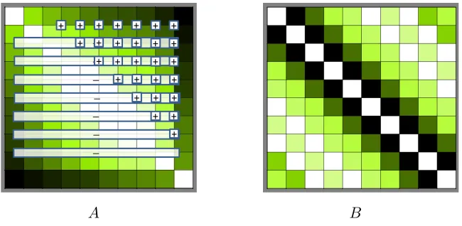
According to Observation 2.9, ifπ∗ is an optimal solution ofQAP(A, B) with a symmetric monotone anti-Monge matrixAand an up-benevolent matrixB, thenidis an optimal solution of QAP(Aπ∗_{, B). In particular this clearly holds for A = ¯R}(p,q) _{with 1 ≤ p ≤q ≤n. Notice} that, in general, the permuted matrix Aπ∗ is not an anti-Monge matrix any more. Figure 6 illustrates the effect of permuting the 10×10 matrix ¯R(2,7) according to permutation π∗.

Let us denote by ¯R(p,q,π∗)the matrix obtained by permuting ¯R(p,q)according to the Supnick permutation π∗, 1≤p≤q≤n.3

By taking a closer look at the matrices ¯R(p,q,π∗) we can observe that they are given as follows

¯

r(p,q,π

∗₎

ji = ¯r

(p,q,π∗)

ij =



     

     

2 dn−₂pe+ 1≤i, j≤n− bn−₂pc

1 dn−₂pe − bq−₂pc+ 1≤i≤ dn−₂pe,dn−₂pe+ 1≤j ≤n− bn−₂pc

1 dn−₂pe+ 1≤i≤n− bn−₂pc, n− bn−₂pc+ 1≤j≤n− bn−₂pc+dq−₂pe 0 otherwise

3

A Aπ∗

Figure 6: Illustration of permuted matrices: A := ¯R(2,7) - a 10×10 symmetric monotone anti-Monge matrix; Aπ∗ _{- a permuted anti-Monge matrix: four anti-Monge inequalities are}

violated; the quadruples of entries involved in the violated inequalities are the ones around the “minus” signs, respectively.

for 1≤i≤j ≤n.

Thus the non-zero entries of these permuted matrices build a kind of a cross with entries equal to 2 at the center of the cross and entries equal to 1 at the arms of the cross (see also Figure 6). Now consider a transformation of the matrix ¯R(p,q,π∗) realized by sliding the cross of non-zero entries along the diagonal such that its arms do not wrap around the border of the matrix (they may touch the border but should not wrap around it). This transformation is done by permuting (the rows and columns of)R(p,q,π∗)according to a shiftσu ∈ Snof the form

hu, u+ 1, . . . , n,1, . . . , u−1iwith 1< u≤ dn−₂pe − bq−₂pc+ 1, orn− bn−₂pc+dq−₂pe+ 1≤u≤n.

Let us denote by C(p,q,u) _{the matrix obtained from R}(p,q,π∗) _{by permuting it according to}

σu with u as described above. Obviously Z(C(p,q,u), B, id) = Z( ¯R(p,q,π

∗₎

, B, id) holds for all 1≤p≤q≤n, for all possible values ofuas given above, and for any Toeplitz matrixB. This is due to the facts that a) the permutationσushifts non-zero entries of ¯R(p,q)along lines parallel

to the main diagonal and b) a Toeplitz matrix has constant entries along any line parallel to the main diagonal. Combined with the third statement of Observation 2.9 the above equation shows thatidis also the optimal solution ofQAP(C(p,q,u), B). This observation motivates the following definition.

Definition 3.7 Let C(p,q,u) be the matrix obtained from R(p,q,π∗) by permuting it according to σu, where σu ∈ Sn is a shift of the form hu, u + 1, . . . , n,1, . . . , u−1i with 1 < u ≤

dn−₂pe − bq−₂pc+ 1or n− bn−₂pc+dq−₂pe+ 1≤u≤n. A symmetric n×nmatrixA0 is called a

permuted-shifted anti-Monge matrix (PS anti-Monge matrix), if it can be obtained as a conic combination ofR(p,q,π∗)and matricesC(p,q,u), for1≤p≤q≤n, and1< u≤ dn−₂pe−bq−₂pc+1 or n− bn−₂pc+dq−₂pe+ 1≤u≤n.

it by −1 and by then adding a sum matrix to it (which can also be the zero matrix, i.e. the matrix containing only entries equal to zero). See Figure 7 for a graphical illustration of PS anti-Monge and PS Monge matrices.

Summarizing we have proved the following result (recall that a sum matrix is both Monge and anti-Monge):

Theorem 3.8 QAP(A, B) with a PS anti-Monge matrix A and an up-benevolent Toeplitz matrixB is solved to optimality by the identity permutation.

Notice that this result is a strict generalization of the result of Burkard & al. [5], because the permutation of a PS-anti-Monge matrix by the inverse (π∗)−1 of the Supnick permutation

π∗ does not yield an anti-Monge matrix in general.

Finally observe that, clearly, the n×n PS anti-Monge matrices form also cone whose extremal rays are the matrices C(p,q,u) with 1 ≤ p ≤q ≤ n, 1 < u ≤ dn−₂pe − bq−₂pc+ 1, or

n− bn−₂pc+dq−₂pe+ 1≤u≤n. Thus these extremal rays build a three parametric family of matrices in contrast to the extremal rays of the (symmetric) monotone anti-Monge matrices which build a two parametric family.

Since the equality Z(A, B, π) = Z(−A,−B, π) trivially holds for any permutation π,

QAP(A, B) and QAP(−A,−B) have the same set of optimal solutions. Notice, moreover, that if B is up-benevolent Toeplitz matrix than −B is a down-benevolent Toeplitz matrix. Summarizing we obtain:

Corollary 3.9 QAP(A, B)with a PS Monge matrixAand a down-benevolent Toeplitz matrix

B is solved to optimality by the identity permutation.

A A−

3.3 Combined QAPs

In the previous sections we reviewed known p.s.s. cases of the QAP and proved some new results. Some of the old and new p.s.s. cases use the same special structures, for example the cut matrices in CDW normal form are involved in the old p.s.s. case described in Theorem 2.5 and in the new p.s.s. case described in Theorem 3.4. In this section we show that such old and new p.s.s. cases can be combined into new structures and new p.s.s. cases.

Cut matrices in CDW normal form. Consider a QAP(A, B) where the matrix A

is a conic combination of cut matrices in CDW normal form. Since this matrix is both a Kalmanson and a Robinson matrix, we can combine the old p.s.s. case described in Theorem 2.5 and the new p.s.s. case presented in Theorem 3.4: matrix B can now be chosen to be a conic combination of two matrices, a symmetric monotone anti-Monge matrix and a down-benevolent Toeplitz matrix (see illustration on Figure 8).

A

+

B1 B2

Figure 8: Illustration ofQAP(A, B1+B2) whereA is a conic combination of cut matrices in CDW normal form, B1 is a monotone anti-Monge matrix, B2 is a down-benevolent Toeplitz matrix.

Down-benevolent Toeplitz. By combining the p.s.s. cases described in Theorem 3.4 and in Corollary 3.9 we get a new p.s.s. caseQAP(A, B1+B2), whereAis a down-benevolent Toeplitz matrix, and the second matrix B is a conic combination of matrices which are both Kalmanson and Robinson matrices and a PS Monge matrix (see illustration on Figure 9).

A

+

B1 B2

DW-Toeplitz. Let A be a DW-Toeplitz matrix. Clearly such a matrix A is a special down-benevolent matrix. By definition A is also a symmetric circulant matrix. Consider now a p.s.s. case QAP(A, B) for which the identity is an optimal solution. Since matrix A has a circular structure, the identity is still an optimal solution of QAP(A, B(u)), where B(u) is obtained from B by applying to it an arbitrary cyclic shift according to some permutation

σu =hu, u+ 1, . . . , n,1, . . . , u−1i, for any 1≤u≤n(u= 1 yields the identity permutation as

a trivial cyclic shift). In particular consider aQAP(A, B), where A is a DW-Toeplitz matrix and B =−R¯(p,q), for some 1≤p ≤q ≤n. This QAP is solved to optimality by the identity permutation as stated in Theorem 3.5. But then the identity permutation is also an optimal solution of QAP(A,−C(p,q,u)), where −C(p,q,u) is obtained fromB =−R¯(p,q) by permuting it according to σu, 1≤ u ≤n. Thus we can extend the class of PS Monge matrices defined in

Section 3.2 and obtain the class of thecyclic PS Monge matrices, which is the class of matrices obtained by first permuting−R(p,q)according toπ∗and then by permuting the resulting matrix according to a cyclic shiftσu, 1≤p≤q≤n and 1≤u≤n.

Figure 10 illustrates such cyclic PS Monge matrices.

We can define now a new combined special case of the QAP solved to optimality by the identity permutation, namely QAP(A, B1+B2), where A is a DW-Toeplitz matrix, and B is a conic combination of a Kalmanson matrix and a cyclic PS monotone Monge matrix (see the illustration in Figure 11).

i1 j1

L1i1j1k

i2 j2 j3 i3

L1i2j2k _L1i3j3k

Figure 10: Illustration of extremal rays which generate the cone of Circular PS Monge matrices.

4

Conic representation of specially structured matrices

4.1 Cut weights and specially structured matrices

In this section, we investigate the structure of matrices which are both Kalmanson and Robin-son matrices. We show that any matrix in this class can be represented as a sum of a constant matrix and a conic combination of cut matrices.

We use the alternative definition of Kalmanson matrices, see Definition 2.6. Consider special cut matrices A(k,l) = (aij), 1≤k < l≤n, containing one block of size (k−l+ 1) with

A

+

B1 B2

Figure 11: Illustration ofQAP(A, B1+B2) where A is a DW-Toeplitz matrix, B1 is a cyclic PS monotone Monge matrix,B2 is a Kalmanson matrix.

It can be easily observed that the matrices A(k,l) fulfill the inequalities (6) and (7) and are therefore Kalmanson matrices. Notice moreover that for any n×n cut matrix A(k,l)_, 1< k < l < n, there is only one strict inequality in (6), namely

ak−1,l+ak,l+1> akl+ak−1,l+1,

whereas all inequalities (7) are fulfilled with equality. Analogously, there is only one strict inequality in (7) for the matricesA(1,k−1) and A(k,n), 2< k < n, namely

ak−1,1+akn< ak1+ak−1,n,

whereas all inequalities (6) are fulfilled with equality4.

The following lemma shows that any Kalmanson matrix can be represented as a linear combination of a weak sum matrix with cut matricesA(k,l) which can be computed explicitly in terms of simple formulas involving the entries of the considered Kalmanson matrix5. Similar structural properties of Kalmanson matrices in terms of cuts and cut-weights have also been studied in [2] and [15]. In both papers though the authors suggest algorithms for calculating the cut-weights while we provide simple analytical expressions for them.

Lemma 4.1 A symmetric n×n matrix C is a Kalmanson matrix if and only if it can be represented as a linear combination of a weak sum matrixS and cut matrices A(k,l) as follows

C=S+

n−3

X

i=1

n−1

X

j=i+2

δi+1,jA(i+1,j)+ n−2

X

i=2

(αiA(1,i)+βiA(i+1,n)). (10)

The coefficients of the linear combination, the so-called cut weights, are given as δi+1,j =

(−ci,j+1−ci+1,j +cij +ci+1,j+1), αi = ci+1,1−ci,1, βi = cin−ci+1,n and fulfill δi+1,j ≥ 0,

αi+βi≥0.

4_{Notice that we refrain from using superscripts in the entries of the matrixA}(k,l)_{; this yields to a slightly}

inconsistent but less incumbent notation.

5

Proof. It can easily be checked that any weak sum matrix, a cut matrixA(k,l), and a linear combinationαiA(1,i)+βiA(i+1,n) with αi+βi≥0 are Kalmanson matrices, and therefore any

matrix given as in (10) is a Kalmanson matrix.

Assume now that C is a Kalmanson matrix. Let i and j, 1 ≤ i < i+ 2 ≤ j < n−1 be two indices, such the corresponding inequality in (6) is strict, i.e.ci,j+1+ci+1,j < cij+ci+1,j+1 holds. The involved matrix entries are printed in boldface in the illustration below, note that all these entries lie above the main diagonal.

C=         . . .

. . . ci,p . . . ci,j−1 ci,j ci,j+1 . . .

. . . ci+1,p . . . ci+1,j−1 ci+1,j ci+1,j+1 . . .

. . .

. . . cq,p . . . cq,j−1 cq,j cq,j+1 . . .

. . .        

Setδi+1,j :=−ci,j+1−ci+1,j+cij+ci+1,j+1 >0 and consider the matrixC0=C−δi+1,jA(i+1,j),

represented schematically below (to simplify the illustration we use the notationδ :=δi+1,j):

C0 =

                

c11−δ . . . c1,i−δ c1,i+1−δ . . . c1j−δ c1,j+1−δ . . . c1,n−δ

. .. . .. . .. . .. . .. . .. . .. . .. . ..

ci,1−δ . . . ci,i−δ ci,i+1−δ . . . ci,j−δ ci,j+1−δ . . . ci,n−δ

ci+1,1−δ . . . ci+1,i−δ ci+1,i+1 . . . ci+1,j ci+1,j+1−δ . . . ci+1,n−δ

. .. . .. . .. . .. . .. . .. . .. . .. . ..

cj,1−δ . . . cj,i−δ cj,i+1 . . . cj,j cj,j+1−δ . . . cj,n−δ

cj+1,1−δ . . . cj+1,i−δ cj+1,i+1−δ . . . cj+1,j−δ cj+1,j+1−δ . . . cj+1,n−δ

. .. . .. . .. . .. . .. . .. . .. . .. . ..

cn,1−δ . . . cn,i−δ cn,i+1−δ . . . cn,j−δ cn,j+1−δ . . . cn,n−δ

                

Notice that in matrixC0= (c0_ij) we havec0_i,j+1+c_i0_+1,j=c0_ij+c0_i+1,j+1. Moreover the status of the other inequalities in (6) does not change, meaning that all inequalities are still fulfilled by matrix C0 and only the inequalities which were strictly fulfilled by C are strictly fulfilled by C0. Finally it is also easy to see that C0 fulfills inequalities (6). Hence C0 is a Kalmanson matrix, and we check again whether there is a pair of indices for which the corresponding inequality in (6) is strict. If yes, we perform an analogous transformation as the one described above by defining the corresponding δ-coefficient and subtracting from C0 the corresponding cut matrix multiplied by that coefficient. We repeat this process, updateC0 in every step, and eventually obtain a Kalmanson matrixC0 which fulfills all inequalities (6) by equality.

Leti, 2≤i≤n−2, be an index such that ci1+ci+1,n< ci+1,1+cin: C=     . . .

ci1 ci2 . . . 0 . . . ci,n−1 cin

ci+1,1 ci+1,2 . . . 0 . . . ci+1,n−1 ci+1,n

. . .



  

Set αi = ci+1,1−ci,1, βi = cin−ci+1,n. Clearly αi +βi > 0 holds, due to ci1+ci+1,n <

ci+1,1+cin. Consider the matrix C0 =C−αA(1,i)−β A(i+1,n) whereα:=αi,β :=βi:

C0=

         

c1,1−β . . . c1,i−β c1,i+1−α−β . . . c1,n−α−β

. .. . .. . .. . .. . .. . ..

ci,1−β . . . ci,i−β ci,i+1−α−β . . . ci,n−α−β

ci+1,1−α−β . . . ci+1,i−α−β ci+1,i+1−α . . . ci+1,n−α

. .. . .. . .. . .. . .. . ..

cn,1−α−β . . . cn,i−α−β cn,i+1−α . . . cn,n−α

         

It can be easily checked that c0_i1 +c0_i+1,n = c0_i+1,1 +c0_in, that all inequalities (6) remain fulfilled with equality, and that the status of the other inequalities in (7) does not change, meaning that all these inequalities are still fulfilled by matrix C0 and only those inequalities among them which were strictly fulfilled byC, are strictly fulfilled byC0. As long as there are inequalities (7) strictly fulfilled by C0 we apply a transformation as above on C0 and update

C0. So eventually we get a transformed matrix where all inequalities (6), (7) are fulfilled with equality. Such a matrix is a weak sum matrix, as shown in Lemma 4.2 below, and this

completes the proof.

Lemma 4.2 Let C be an n×n Kalmanson matrix for which all inequalities in (6) and (7) are fulfilled with equality. Then C is a weak sum matrix.

Proof. We show that the entries of matrix C= (cij) can be represented as

cij =γi+γj fori, j ∈ {1,2, . . . , n},i < j, and some γ = (γi)∈Rn. (11)

First, we show how to calculateγi,i= 1, . . . , n, and then we prove that the above representation

is valid.

By solving the simple system of linear equationsγ1+γ2 =c12,γ1+γ3 =c13, andγ2+γ3 =c23 we get

γ1 = (c12+c13−c23)/2, γ2 = (c12+c23−c13)/2, γ3 = (c13+c23−c12)/2. (12)

The remaining γi, i∈ {4,5, . . . , n} are calculated as γi :=c1i−γ1. We have now c1j =cj1 =

γ1+γj, forj= 2, . . . , n, and c23=c32=γ2+γ3.

Next we show thatcij =γi+γj holds for the remaining pairs of indices (i, j), i.e. for (i, j)∈

following order (2,4),(2,5), . . . ,(2, n), (3, n),(3, n−1), . . . ,(3,4), . . . ,(4, n), . . . ,(4,5),(n−1, n). For (2,4) we obtain by applying (in)equality (6) and equalities (12) c24 = c23+c14−c13 =

γ2 +γ3 +γ1 +γ4 −γ1 −γ3 = γ2 +γ4. Observe that for each of the remaining entries cjl

there is always one of the (in)equalities (6) or (7) which involves cjl and three other entries

cik, cil, cjk which have been considered before to cjl in the above specified order. Thus for

those three entries the corresponding equalities (11) hold: cik = γi+γk, cjk = γj +γk, and

cil =γi+γl. Fromcik+cjl =cil+cjk and the above three equalities we getcjl=cjk+cil−cik =

γj +γk+γi+γl−γi−γk=γj+γl, and this completes the proof.

Next we give a characterization of Kalmanson matrices which are also Robinson matrices. This characterization involves again the special cut matricesA(k,l).

Lemma 4.3 A symmetric n×n matrix C is both a Kalmanson and a Robinson matrix if and only if it can be represented as a conic combination of a weak constant matrix Z and cut matrices A(k,l) as follows

C=Z+

n−3

X

i=1

n−1

X

j=i+2

δi+1,jA(i+1,j)+ n−1

X

i=2

αiA(1,i)+ n−2

X

i=1

βiA(i+1,n), (13)

where δi+1,j := (−ci,j+1 −ci+1,j +cij +ci+1,j+1), for 1 ≤ i ≤ n−3, i+ 2 ≤ j ≤ n−1,

αi := ci+1,1 −ci,1, for 2 ≤ i ≤ n−1, βi := cin−ci+1,n, for 1 ≤ i≤ n−2, and δi+1,j ≥ 0,

αi ≥0, βi≥0.

Proof. The proof of the “if”-part of the lemma is straightforward; just observe that all matrices in the conic combination are Kalmanson and Robinson matrices and that a conic combination preserves the Kalmanson and Robinson properties because all of them are defined in terms of inequalities involving the entries of the matrix.

We prove now the “only if”-part. SinceC is a Kalmanson matrix it has a representation as stated by Lemma 4.1 in (10). Observe that (10) and (13) differ on the first summand, which is a weak sum matrix in (10) and constant matrix in (13), and on the range of summation for the third and the fourth summand (combined in one single summand in (10)). We go through the procedure applied in Lemma 4.1 and show the matrix C0 resulting after each transformation step is again a Robinson matrix. The non-negativity of the coefficientsαi andβi in (10) would

then follow directly from the definition of a Robinson matrix.

Consider first a transformation of the type C0 = C −∆A(i+1,j), where ∆ = δi+1,j. We

claim thatcip−∆≥ci+1,p for all p=i+ 2, . . . , j. Let Λp =cip−ci+1,p,p=i+ 2, . . . , j+ 1.

Since C is a Robinson matrix, we have Λp ≥0. Since C is a Kalmanson matrix, we have

cip+ci+1,j−ci+1,p−ci,j = Λp−Λj ≥0 and Λp ≥Λj. Clearly ∆ = Λj−Λj+1 and therefore

cip−∆−ci+1,p= Λp−Λj+ Λj+1 ≥0, which proves the claim. The claim thatcq,j+1−∆≥cqj

for allq =i+ 1, . . . , j−1 can be proved in a similar way. So the new matrixC0 is a Robinson matrix.

Consider now a transformation of the typeC0 =C−αiA(1,i)−βiA(i+1,n), for 2≤i≤n−2.

is thatZ =S−αn−1A(1,n−1)−β1A(2,n) is a weak constant matrix, whereS is the weak sum matrix in the presentation (10).

Since every transformation step results in a Robinson matrix, as shown above, the weak sum matrix S resulting after the last transformation in the proof of Lemma 4.1 is a Robinson matrix, too. It is easily seen that a symmetric weak sum matrix S= (sij) withsij =γi+γj,

for 1 ≤ i < j ≤ n, is a Robinson matrix, if and only if γ1 ≥ γ2 = . . . = γn−1 ≤ γn.

Indeed s1j =γ1+γj ≤ s1,j+1 = γ1 +γj+1 implies γj ≤γj+1 , for j ∈ {2,3, . . . , n−1}, and

si−1,n =γi−1+γn≥si,n=γi+γn, impliesγi−1 ≥γi, fori∈ {2,3, . . . , n−1}.

After the last transformation the equalitiessn,1−sn−1,1=γn−γn−1 =cn,1−cn−1,1=αn−1 and s1,n−s2,n=γ1−γ2=c1,n−c2,n =β1 clearly hold. Observe finally that

S−(γn−γn−1)×A(1,n−1)−(γ1−γ2)×A(2,n)=S−αn−1A(1,n−1)−β1A(2,n)

is a weak constant matrix (with all non-diagonal elements equal to 2γ2), which completes the

proof.

By applying the above lemma to compute the coefficients of the conic combination for a cut matrix (which is a Kalmanson and a Robinson matrix) we obtain

Corollary 4.4 LetC be a cut matrix withmblocks such thatkof them (k≤m) contain more than one element. Let the correspondingkrow and column blocksI1, I2, . . . , Ik,|Ij|>1, ∀j, of

C be given asI1 ={i1= 1, . . . , j1},I2={i2, . . . , j2}, . . . ,Ik={ik, . . . , jk}, whereil≥jl−1+ 1

andil < jl, for 1≤l≤k. ThenCcan be represented asC=Z+Pl_l=₌₁kA(il,jl), whereZ = (zij) withzij =−(k−1)for i6=j.

4.2 Recognizing conic combinations of cut matrices in CDW normal form

As mentioned in Section 3.3 a combined p.s.s. case of the QAP arises if one of the coefficient matrices is a conic combination of cut matrices in CDW normal form and the other one is a conic combination of a symmetric anti-Monge matrix and a down-benevolent Toeplitz matrix. Thus, given a matrix C which is both a Kalmanson matrix and a Robinson matrix, it is a question of interest whether the matrix can be represented as a conic combination of cut matrices in CDW normal form. Notice that every cut matrix in CDW normal form is both a Robinson and a Kalmanson matrix but not vice versa. Notice moreover that a weakly constant matrix with zeroes on the diagonal and constant K∈_Relsewhere can be obtained by multiplying with K

a special cut matrix in CDW normal form with all blocks of length one. In order to formulate a simple rule for recognizing this special subclass of Kalmanson (and Robinson) matrices, we will associate to every (Kalmanson and Robinson) matrix C an n×n symmetric cut-weight matrixD(C) = (dij) with dij :=δij =ci−1,j+ci,j+1−cij−ci−1,j+1 for 2≤i < j ≤n−1, and

d1i :=αi =ci+1,1−ci1,i= 2, . . . , n−1,din :=βi−1 =ci−1,n−cin, i= 2, . . . , n−1. Observe

that the coefficientsδij,αi andβi−1 are as defined in Lemma 4.3. The elements which are not defined are irrelevant for further considerations, and are set to be zeros.

Consider a cut matrix in CDW normal form. LetIl={il, . . . , jl}, 1≤l≤k, be itskblocks

and il =jl−1+ 1, for 2≤l≤k. Clearly, the corresponding cut-weight matrix contains onlyk non-zero elementsdil,jl = 1, 1≤l≤k, exactly one for each block.

Next we will represent an n×ncut matrix in CDW normal form by a directed graph with

n+ 1 nodes on a line, and edges determined in terms of the cut-weight matrix, as follows. Let the nodes be labeled by{1,2, . . . , n+1}, increasing from the left to the right. For each non-zero entrydi1,j1 = 1, 1≤l≤k, of the cut-weight matrix we introduce an edge that connects nodes

i1 and j1+ 1 and is directed from i1 toj1+ 1, hence from the left to the right; see Figure 12 for an illustration. Letkbe the vertex with the smallest index having a positive degree. Then the degree of kequals 1, i.e. deg(k) = 1 and every nodei∈ {k+ 1, . . . , n} has degree 0 or 2, whereas the degree of node n+ 1 equals 1. Furthermore notice that for every directed edge (i, k) in this graph i+ 1 < k holds. For such an edge we will say that it enters node k and leaves nodei. Finally notice that if there is an edge entering a nodek≤n−1, then the edge leaving node kis at least as long as the edge entering k, where the length of an edge (i, k) is given as k−i, for i+ 1< k. A directed graph with all these properties is called a multi-cut graphand is formally defined as follows.

Definition 4.5 A directed graph G= (V, E) with node set V ={1,2, . . . , n+ 1} and edge set

E={(ip, ip+1) : 1≤p≤ |E|}, where all edges are directed from the node with the smaller index

to the node with larger index, with the following properties

(a) Let i1:=k be the vertex with the smallest index such thatdeg(k)>0. Then deg(k) = 1,

deg(v) ∈ {0,2}, for v ∈ {k+ 1, k+ 2, . . . , n} and deg(n+ 1) = 1, wheredeg(v) denotes the degree of v in G.

(b) The length of every edge (ip, ip+1) ∈E is not smaller than 2, i.e. ip+1−ip ≥2, for all

1≤p≤ |E|.

(c) The inequalities ip+1−ip ≤ip+2−ip+i hold for all 1≤p≤ |E| −1. is called a cut-weight graph.

It is straightforward to see that the symmetric matrixD= (dij) constructed in relationship

with an arbitrary cut-weight graph G by setting its entriesdip,ip+1 = 1 for any edge index p,

1≤p≤ |E|anddij = 0 otherwise, for alli < j, is the cut-vertex matrixD(C) =:Dof ann×n

block matrix C in CDW normal form. C has k−1 +|E| blocks which are given as Ij ={j},

forj < k=i1, and Ik−1+p ={ip, ip+ 1, . . . , ip+1−1}, for 1≤p≤ |E|.

So to every block matrix in CDW normal form a cut-weight graph can be associated, and vice versa, to every cut-weight graph a block matrix in CDW normal form can be associated, as above.

Consider now a conic combinationA=Pq

p=1αpAp of (Kalmanson and Robinson) matrices

Ap, for 1 ≤ p ≤ q. Clearly the cut-weight matrix of the linear (conic) combination can be

obtained as a conic combination of the cut-weight matrices of the summands, i.e. D(A) =

Pq

More precisely for every two nodes iand k+ 1, 1≤i≤n−2 and i+ 2≤k+ 1≤n+ 1, the number of directed edges (i, k+ 1) equals Pq

p=1αpd

(p)

i,k where d

(p)

i,k is the corresponding entry

of D(Ap), for 1 ≤p ≤ q. Consequently for each edge of length x entering a node k, there is

one edge of length at leastx leaving node k. Let us denote byE−(k+ 1, x) andE+(k+ 1, x) the number of edges of length at least x entering or leaving the node k+ 1, respectively. Then, clearly the number of edges of length at leastxentering nodek+ 1 does not exceed the number of edges of length at least x leaving node k+ 1, thus E−(k+ 1, x) ≤ E+(k+ 1, x), holds for 3≤k+ 1≤n−1, 2≤x ≤k. By considering thatE−(k+ 1, x) =Pk+1−x

i=1 dik and

E+(k+ 1, x) =Pn

j=k+1+x−1dk+1,j, we get: k+1−x

X

i=1

dik ≤ n

X

j=k+1+x−1

dk+1,j, for 2≤k+ 1≤n−2 and 2≤x≤k. (14)

Notice that by settingl:=k+ 1−x inequalities (14) can be equivalently written as

l

X

i=1

dik≤ n

X

j=2k+1−l

dk+1,j (15)

for k = 2, . . . , n−2 and l = 1, . . . , k−1. The right-hand sum in (15) is considered to be zero if 2k+ 1−l > n. This in particular means that dik = 0 for k = dn/2e, . . . , n−1 and

i= 1, . . . ,2k−n.

It turns out that the later inequalities fulfilled by the entries of the cut-weight matrix

D := D(A) of some matrix A are not only necessary, but also sufficient for A to be a conic combination of cut matrices in CDW normal form, i.e. for A to be representable as A =

Pq

p=1αpAp, with cut matricesAp, 1≤p≤q, in CDW normal form.

1 2 3 4 5 6 7 8 9 10 11 12 13

Figure 12: Illustration of the graph representation of a 12×12 cut matrix in CDW normal form with the blocks {2,3}, {4,5}, {6,7,8}, and {9,10,11,12}. All edges are directed from left to right.

Proof. The proof of the necessary condition is trivial. Let A =Pq

p=1αpAp be an n×n matrix which is a conic combination ofn×ncut matricesAp in CDW normal form, 1≤p≤q.

Let D(A) = (dij) be the cut-weight matrix of A. Assume for simplicity (and without loss

of generality) that the weight coefficients αp, 1 ≤ p ≤ q, are natural numbers. Then, since

D(A) = Pq

p=1αpD(Ap), the entries dlk, 1 ≤ l, k ≤ n, of D(A) are also natural numbers.

Inequalities (14), and consequently also inequalities (15), are obviously fulfilled due to the construction of the directed multigraph corresponding to A.

Assume now that the entries of the cut-matrixD(C) of an integer Kalmanson and symmet-ric matrixC satisfy the inequalities (15). Similarly as in the discussion preceding the theorem we build an auxiliary directed multigraph with n+ 1 nodes {1,2, . . . , n+ 1} and dij edges

directed from ito node j+ 1 for each dij >0 and j > i. We refer to this multigraph as the cut-weight multigraph of matrix C.

We build a conic representation of C as follows. We start with node n+ 1 in the cut-weight multigraph, and build a path from the right to the left by choosing in the first step an (reversed) edge (ik−1, ik = n+ 1) with the largest length. Then in each following step

p >1 we construct a longest edge (ik−p, ik−p+1) with length ik−p+1−ik−p ≤ik−p+2−ik−p+1, as long as such an edge exists. Let the constructed path be P1 := (i1, i2, . . . , ik = n+ 1)

where 1 ≤ i1 < i2 < . . . < ik = n+ 1. Consider now the graph G = (V, E) with vertex

set V = {1,2, . . . , n + 1} and edge set E = {(ip, ip+1) : 1 ≤ p ≤ k−1}. This is clearly a cut-weight graph and hence it can be associated to a cut matrix in CDW normal form as described before the theorem. We denote this matrix by A1. Let α1 be the minimum multiplicity of the edges in pathP1. We removeα1copies ofP1 from the cut-weight multigraph of C and set dip,ip+1−1 := dip,ip+1−1 −αi, for 1 ≤ p ≤ k−1. We show that (14), and

equivalently also (15), remain fulfilled after this update. The update of the coefficientsdij can

only affect inequality (15) for indices k such that k+ 1 is an endpoint of an edge in P1, i.e.

k+ 1 ∈ {i1, i2, . . . , ik−1}. For k+ 1 ∈ {i2, . . . , ik−1} the update of dij results in subtracting

αi from both sides of (15), and hence it does not affect the validity of the inequality. It

remains the case k+ 1 = i1 for i1 > 2. Let ¯E−(i1, x), ¯E+(i1, x) be the values of E−(i1, x) and E+(i1, x), after the update of the coefficients dij, respectively. Thus we have to show

that ¯E−(i1, x) ≤ E¯+(i1, x) holds. Let l1 := i2 −i1 be the length of the first edge in P1. If

x > l1 than ¯E+(i1, x) =E+(i1, x) and ¯E−(i1, x) =E−(i1, x), and since E−(i1, x)≤E+(i1, x) holds, there is nothing to show in this case. If x ≤ l1, ¯E+(i1, x) = E+(i1, x)− α1 and

¯

E−(i1, x) = E−(i1, x). Notice that E−(i1, x) = E−(i1, x+ 1), otherwise P1 could have been prolonged beyond i1. Moreover, E−(i1, x+ 1) ≤ E+(i1, x+ 1) due to the assumption of the theorem, and E+(i1, x+ 1) ≤ E+(i1, x) −α1 = ¯E+(i1, x) because there are at least

α1 edges of length x leaving i1. By putting things together we get the required inequality ¯

E−(i1, x)≤E¯+(i1, x).

The path construction and the corresponding update of the coefficient dij can be then

inductively repeated as long as possible, while (15) remains an invariant during this process and in every stepi,i∈_N, a cut matrixAi in CDW normal form is identified. Ai corresponds

to the pathPi constructed in thei-th step. Ifαi is the minimum multiplicity of the edges in

Pi thenαiPi is a summand of the required conic combination. This process is finite because

terminates when there are no edges entering node n+ 1 any more, say after t steps. We claim that after the t-th step, there are no more edges in the cut-weight multigraph at all. This means that the actual coefficients dij fulfill dij = 0 for all i < j, which implies that the

matrixC is transformed into a weak constant matrix Z by subtractingPt

p=1αpAp, and thus

C=Z+Pt

p=1αpAp holds for the original matrixC.

Now let us prove the claim. Assume by contradiction that after t transformation steps there is no edge entering node n+ 1 in the cut-weight multigraph while there is still at least one edge in the graph. Let j be the largest node index such that there is an edge enteringj. Then j ≤ n according to our assumption. The inequalities (15) have to be fulfilled because they are an invariant of the transformation process. In particular, 1 ≤ E−(j,1) ≤ E+(j,1) must hold. This implies the existence of an edge leavingj, and hence entering some node with an index strictly larger thanj. This contradicts the choice ofj and completes the proof of the

claim.

An illustrative example. Consider the matrix C which is in the class of Kalmanson and Robinson matrices: C=        

0 1 2 3 3 3

1 0 2 3 3 3

2 2 0 2 3 3

3 3 2 0 2 2

3 3 3 2 0 1

3 3 3 2 1 0

       

We first illustrate the proofs of Lemmas 4.1 and 4.3 and show how to represent C as sum of a conic combination of cut matricesAkl with a weak constant matrix.

Note that for matrixC there is only one strict inequality in system (6)c25+c34< c24+c35, and three strict inequalities in system (7): ci1+ci+1,6 < ci6+ci+1,1 with i= 2,3,4.

We first eliminate the strict inequality c25 +c34 < c24 +c35 by subtracting from C the cut matrixA34 multiplied by δ34 =c24+c35−c25−c34 =d24 = 1. The transformed matrix

C0 =C−A34 is given as follows.

C0=C−A34=

       

0 0 1 2 2 2

0 0 1 2 2 2

1 1 0 2 2 2

2 2 2 0 1 1

2 2 2 1 0 0

2 2 2 1 0 0

       