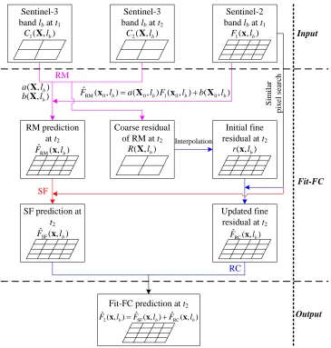
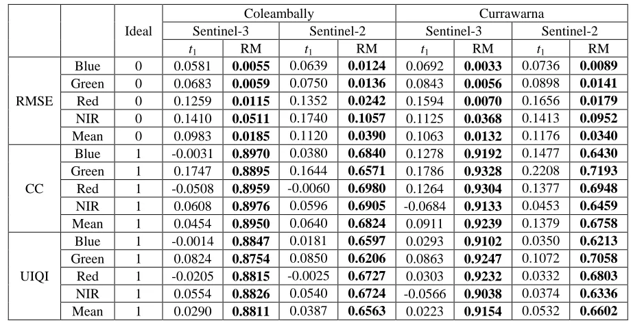
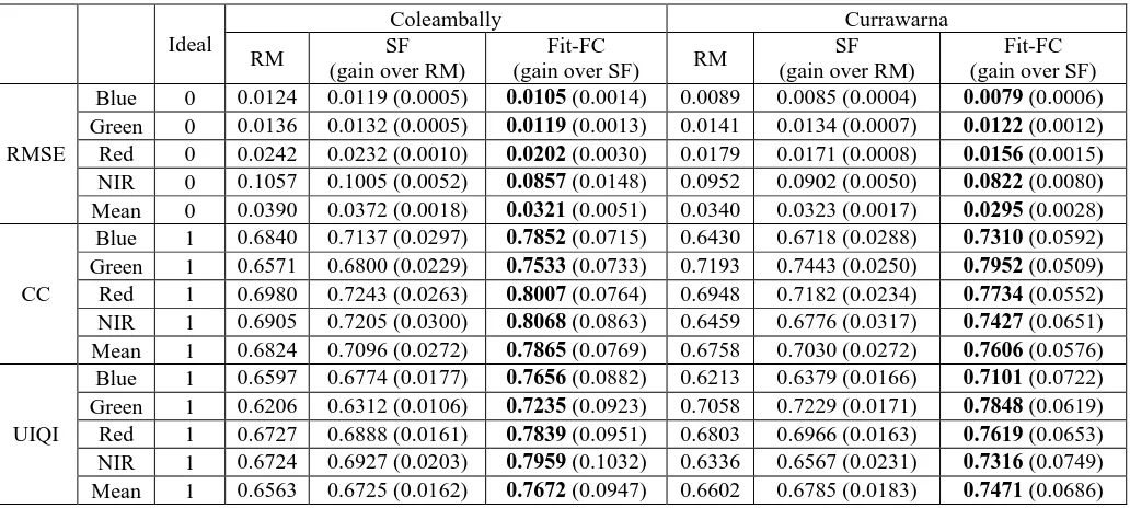
Spatio temporal fusion for daily Sentinel 2 images

With cloud and managed security services, integrated technologies and a team of security experts, ethical hackers and researchers, Trustwave enables businesses to transform the

Rajshahi City Corporation area is divided into four zones for comparative view of existing pedestrian planning condition such as Residential Zone, Commercial zone, Recreational

JBIC signed on July 30, 2020 a loan agreement, in project financing, amounting to up to USD265 million (JBIC portion), with Reliance Bangladesh LNG & Power Limited (RBPL) in

Variables representing board behavior characteristics, namely, ratio of shares owned by the board, board meeting frequency within a year, and the number of independent

In this study we tested the allele-pyramiding approach for Pm3 , a coiled-coil NLR-coding gene that mediates race-specific resistance against powdery mildew ( Blumeria graminis

power to regulate interstate commerce to prevent a private motel from discriminating on the basis of race, color, religion, or national origin. The Motel refused to rent rooms

Corporate paternalism relied on top-down corporate control that extended into nearly every aspect of the industrial system from the water rights that powered the mills to the

Service Design Service Loose Coupling minimizes dependencies Service Abstraction minimizes the availability of meta information Service Compos ability maximizes