Scaling up dynamic optimization problems : a divide and conquer approach

(1)

warwick.ac.uk/lib-publications

Manuscript version: Author’s Accepted Manuscript

The version presented in WRAP is the author’s accepted manuscript and may differ from the

published version or Version of Record.

Persistent WRAP URL:

http://wrap.warwick.ac.uk/113902

How to cite:

Please refer to published version for the most recent bibliographic citation information.

If a published version is known of, the repository item page linked to above, will contain

details on accessing it.

Copyright and reuse:

The Warwick Research Archive Portal (WRAP) makes this work by researchers of the

University of Warwick available open access under the following conditions.

Copyright © and all moral rights to the version of the paper presented here belong to the

individual author(s) and/or other copyright owners. To the extent reasonable and

practicable the material made available in WRAP has been checked for eligibility before

being made available.

Copies of full items can be used for personal research or study, educational, or not-for-profit

purposes without prior permission or charge. Provided that the authors, title and full

bibliographic details are credited, a hyperlink and/or URL is given for the original metadata

page and the content is not changed in any way.

Publisher’s statement:

Please refer to the repository item page, publisher’s statement section, for further

information.

(2)

Scaling Up Dynamic Optimization Problems:

A Divide-and-Conquer Approach

Danial Yazdani, Mohammad Nabi Omidvar, J¨urgen Branke, Trung Thanh Nguyen, and Xin Yao

Abstract—Scalability is a crucial aspect of designing efficient algorithms. Despite their prevalence, large-scale dynamic opti-mization problems are not well-studied in the literature. This paper is concerned with designing benchmarks and frameworks for the study of large-scale dynamic optimization problems. We start by a formal analysis of the moving peaks benchmark and show its nonseparable nature irrespective of its number of peaks. We then propose a composite moving peaks benchmark suite with exploitable modularity covering a wide range of scalable partially separable functions suitable for the study of large-scale dynamic optimization problems. The benchmark exhibits modularity, heterogeneity, and imbalance features to resemble real-world problems. To deal with the intricacies of large-scale dynamic optimization problems, we propose a decomposition-based coevolutionary framework which breaks a large-scale dynamic optimization problem into a set of lower dimensional components. A novel aspect of the framework is its efficient bi-level resource allocation mechanism which controls the budget assignment to components and the populations responsible for tracking multiple moving optima. Based on a comprehensive empirical study on a wide range of large-scale dynamic op-timization problems with up to 200 dimensions, we show the crucial role of problem decomposition and resource allocation in dealing with these problems. The experimental results clearly show the superiority of the proposed framework over three other approaches in solving large-scale dynamic optimization problems.

Index Terms—dynamic optimization problems, large-scale op-timization problems, decomposition, multi-population, computa-tional resource allocation, cooperative coevolutionary.

I. INTRODUCTION

Change is an inescapable aspect of natural and artificial systems, and adaptation is central to their resilience [1], [2]. Optimization problems are no exception to this maxim. Indeed,

This work was supported in part by a Deans Scholarship by Faculty of Engineering and Technology, LJMU, a Newton Institutional Links grant no. 172734213, funded by the UK BEIS and delivered by the British Council, a NRCP grant no. NRCP1617-6-125 delivered by Royal Academy of Engineering, two EPSRC grants (nos. EP/P005578/1 and EP/J017515/1). Xin Yao was supported by a Royal Society Wolfson Research Merit Award and Honda Research Institute Europe.

D. Yazdani and T. T. Nguyen are with the Liverpool Logistics, Offshore and Marine Research Institute, Department of Maritime and Mechanical Engineering, Liverpool John Moores University, Liverpool L3 3AF, United Kingdom (e-mails: [email protected], [email protected]).

M. N. Omidvar and X. Yao are with the Center of Excellence for Research in Computational Intelligence and Applications (CERCIA), School of Computer Science, University of Birmingham, Birmingham B15 2TT, U.K. (e-mail: [email protected], [email protected]). Xin Yao is also with the Department of Computer Science and Engineering, Southern University of Science and Technology, Shenzhen 518055, China.

J. Branke is with the Operational Research and Management Sciences Group in Warwick Business school, University of Warwick, Coventry CV4 7AL, United Kingdom (email: [email protected]).

The first two authors contributed equally to this work.

viability of businesses and their operational success depends heavily on their effectiveness in responding to a change in the myriad of optimization problems they entail. For an optimization problem, this boils down to the efficiency of an algorithm to find and maintain a quality solution to an ever changing problem.

Ubiquity of dynamic optimization problems (DOPs) [3] demands extensive research into design and development of algorithms capable of dealing with various types of change [4]. These are often attributed to a change in the objective function, its number of decision variables, or constraints. Despite the large body of literature on dynamic optimization problems and algorithms, little attention has been given to their scal-ability. Indeed, the number of dimensions of a typical DOP studied in the literature rarely exceeds twenty. This is contrary to the emergence of high-dimensional dynamic optimization problems such as deep online learning [5]. Deep learning problems are large-scale by nature and the arrival of new training data makes online learning a dynamic problem. Online clustering of high-dimensional data is another example of a large-scale dynamic optimization problem [6], [7]. Many large-scale static optimization problems can also be regarded as dynamic due to unforeseen environmental changes. Large-scale crossing waypoints locating in air route networks is such a problem whose problem space changes by delayed airplanes, breakdowns, and extreme weather conditions [8].

Motivated by rapid technological advancements, large-scale optimization has gained popularity in recent years [9]. How-ever, the exponential growth in the size of the search space, with respect to an increase in the number of decision variables, has made large-scale optimization a challenging task. For DOPs, however, the challenge is twofold. For such problems, not only should an algorithm be capable of finding the global optimum in the vastness of the search space but it should also be able to track it over time. For multi-modal DOPs, where several optima have the potential to turn into the global optimum after environmental changes, the cost of tracking multiple moving optima also adds to the complexity.

(3)

algorithms [16], [17]. Diviand-conquer and problem de-composition techniques have also gained popularity in large-scale global optimization in recent years [18], [19]. However, scalability of dynamic optimization algorithms and the notion of exploiting problem structure are under-explored areas which we set out to study in this paper.

Moving peaks benchmark (MPB) [20] is the most popular benchmark in the field of dynamic optimization. Despite being scalable, MPB’s lack of modularity limits its utility for the study of large-scale DOPs. Real-world problems often exhibit a modular structure with nonuniform imbalance among the contribution of its constituent parts to the objective value [21]. The modularity is caused by the interaction structure of the decision variables resulting in a wide range of structures from fully separable functions to fully nonseparable ones. Most problems exhibit some degree of sparsity in their interaction structure, which can be exploited by optimization algorithms. The imbalance property can be caused as a by-product of modularity or due to the heterogeneous nature of the input variables and their domains. For example, model predictive control (MPC) is a dynamic optimization problem with a wide range of applications in chemical power plants, robotics, and power systems and exhibits modularity and imbalance [22]. In this paper, we formally analyze the standard MPB and show that it is additively nonseparable. We then propose a new benchmark generator by composing several MPBs to account for modularity and imbalance.

In addition to the new benchmark, we draw on advances in large-scale global optimization and propose a decomposition-based framework for large-scale dynamic optimization prob-lems. The idea is to first discover and exploit the underlying structure of a given problem by decomposing it into several components of smaller sizes, and then to tackle the subprob-lems simultaneously. The former can be achieved by a wide range of variable interaction analysis algorithms capable of identifying the underlying structure of a black-box problem with high efficiency and accuracy [18], [19], [23], [24], and the latter can be achieved by means of cooperative coevolution (CC) [25]–[27]. To deal with the imbalance problem, we also devise a new resource allocation policy, which takes the dynamic nature of the problem into account for an economical use of the limited computational resources. We empirically evaluate the proposed framework on a wide range of problem settings to validate the efficacy of various strategies such as problem decomposition, tracking multiple moving optima, and resource allocation. In short, this paper has the following major contributions:

1) A mathematical variable interaction analysis on the MPB benchmark to determine its interaction structure. 2) A large-scale benchmark suite with a modular

heteroge-neous structure allowing for imbalance among its com-ponents.

3) A decomposition-based algorithm for solving large-scale DOPs with a novel resource allocation mechanism.

The organization of this paper is as follows. Section II covers the background information and related work. Sec-tion III contains the analysis of the moving peaks

bench-mark and the details of the proposed large-scale benchbench-mark function generator for DOPs. The details of the proposed decomposition-based algorithm and its resource allocation mechanism is given in Section IV. Section V is concerned with a comprehensive empirical analysis of the proposed algorithm. Finally, Section VI concludes the paper and outlines possible future directions.

II. BACKGROUND ANDLITERATUREREVIEW

DOPs are usually represented as follows:

F(x) =fx, θ(t), (1)

where f is the objective function, x is a design vector, θ(t)

is environmental parameters which change over time andt is the time index with t ∈ [0, T] where T is the problem life cycle. In this paper, like most previous studies in the DOP domain, we investigate DOPs that change discretely over time, i.e., t ∈ {1, . . . , T}. In this type of DOP, the environmental parameters change over time with stationary periods between changes. As a result, for a DOP withT environmental states, we have a sequence ofT static environments:

F(x) =hf(x, θ(1)), f(x, θ(2)), . . . , f(x, θ(T))i, (2)

whereθ(i) denotes the parameters of theith environment.

A. Variable Interaction

Variable interaction or linkage refers to the extent to which the optimum of a variable depends on the values taken by other decision variables. For continuous optimization prob-lems, variable interaction is defined as follows [18]:

Definition 1 (Mei et al. [18]). Let f : Rn → R be a twice

differentiable function. Decision variablesxi and xj interact if a candidate solutionx? exists, such that

∂2f(x?)

∂xi∂xj 6= 0.

Some functions exhibit an underlying interaction structure such that groups of decision variables can be optimized independently. These functions, which are called partially separable, are defined as follows:

Definition 2(Omidvar et al. [21]). A functionf(x)is partially separable withmindependent components iff:

arg min

x

f(x) =arg min

x1

f(x1, . . .), . . . ,arg min xm

f(. . . ,xm)

,

wherex= (x1, . . . , xn)>is a decision vector ofndimensions, x1, . . . ,xmare disjoint sub-vectors ofx, and2≤m≤n. The

function is called fully separable when m=n.

Additive separability is a special type of partial separability, which is defined as follows:

Definition 3 (Omidvar et al. [21]). A function is additively separable if it has the following general form:

f(x) =

m

X

i=1

(4)

Algorithm 1: (x?_{, f}?₎₌ _CC₍_f₎

1 /*Main Framework of CC*/

2 P←randomized initial population;

3 c←randomized initial context vector;

4 //grouping stage

5 G=Grouping(f);

6 //optimization stage

7 whileTermination Condition is Not Satisfieddo

8 forκ= 1to|G| do

9 (P,c) =Optimizer(P,c,Gκ);

10 x?₌_c_;_f?₌_f₍_x?₎_; 11 return(x?_{, f}?₎_;

where fi(·) is a nonseparable subfunction, and m is the number of nonseparable components of f. The definition of

x andxi is identical to what was given in Def. 2.

Definition 4 (Omidvar et al. [21]). A function f(x) is fully nonseparable if every pair of its decision variables interact.

Let us provide two illustrative examples. Given the poly-nomial f(x) = x21 + 3x1x22 + 2x23x34, by applying Def. 1 we can show that _∂x1∂x2∂f(x) = 6x2 which is clearly nonzero when x2 6= 0. Therefore, x1 andx2 interact. Conversely, the quantity _∂x∂f(x)

1∂x3 is identically zero regardless of the choice

of x. Therefore, x1 and x3 are separable. It is clear that the nonlinearity of f(x) is caused by the product terms, resulting in the following interaction groups: {x1, x2} and {x3, x4}. Accordingly, we can rewrite f(x)in terms of two subfunctions as follows: f(x) = f1(x1, x2) + f2(x3, x4). It is therefore clear that f(x) is both partially separable and partially additively separable (Defs. 2 and 3). Another example is g(x) = exp{Pn

i=1x 2

i}. It is clear that all

second-order partial derivatives of g(x) are nonzero except at the origin, which forces all pairs of variables to interact (Def. 4). However, the optimal values for each dimension can still be found independently regardless of the values taken by other dimensions. This makes g(x) fully separable according to Def. 2 wherem=n.

B. Cooperative Coevolution

Cooperative coevolution (CC) has been proposed by Potter and De Jong [25] with the goal of allowing evolutionary algorithms the capacity to solve increasingly complex prob-lems. The idea is based on decomposing a complex problem into subproblems of lower complexity which are coadapted within an evolutionary context. Algorithm 1 shows a high-level representation of CC. In the original implementation of CC, an

n-dimensional problem is decomposed into n 1-dimensional problems each of which is optimized using a given optimizer in a round-robin fashion. In order to assign a fitness to each partial solution in a component, the individuals are evaluated within the context of a complete solution often referred to as the context vector [28].

The round-robin optimization of components assumes a uniform contribution from each component which is often not the case for various reasons [21]. The so-called imbalance

among the contribution of components can be attributed to the following: 1) nonuniform dimensionality of the underlying component functions. 2) component functions with different

landscapes and output ranges. 3) the dynamics of the opti-mizer, its convergence behavior, and stagnation. Contribution-based cooperative coevolution (CBCC) [29], [30] is an im-proved CC framework which addresses the imbalance issue by assigning more resources to components with higher overall contributions. An important aspect of a contribution-aware coevolutionary framework is maintaining an optimal balance between an exploration phase in which the contribution of components is updated, and an exploitation phase in which the most contributing component is optimized. This has resulted in many attempts to design various exploration/exploitation polices [31]–[33].

The original CC framework and its contribution-based counterpart have no explicit means of dealing with variable interactions. They only respond to interactions through the

cooperation of individuals in updating the context vector, which acts as a message passing mechanism. The efficiency of this approach depends on the policy of constructing the context vector [34] as well as its update frequency [35]. To alleviate this problem, many variable interaction analysis algorithms have been proposed with the aim of decomposing a large-scale problem into smaller independent components. There have been many attempts on this [26], [36], among which the differential grouping family of algorithms showed the highest accuracy [18], [19], [23]. Differential grouping (DG) works on the basis of the following theorem:

Theorem 1 (Omidvar et al. [23]). Letf(x) be an additively separable function. ∀a, b1 6= b2, δ ∈ R, δ 6= 0, variables xp

and xq interact if the following condition holds

∆δ,xp[f](x)|xp=a,xq=b1 = ∆6 δ,xp[f](x)|xp=a,xq=b2, (3)

where

∆δ,xp[f](x) =f(. . . , xp+δ, . . .)−f(. . . , xp, . . .), (4)

refers to the forward difference of f with respect to variable

xp with intervalδ.

The quantities in (3) are real-valued numbers; therefore, the equality check cannot be evaluated exactly over the floating-point number field on computer systems. Consequently, the equality check needs to be converted to an inequality check by introducing a sensitivity parameter: |∆(1) ₋_∆(2)_| _>_. Here, ∆(1) and ∆(2) denote the left and right hand side of (3), respectively. In the absence of representation and roundoff errors, can be theoretically set to zero; however, this is not usually the case and the optimal value ofis often a nonzero positive number. This parameterization makes DG sensitive to choices of whose optimal value may vary from function to function and is difficult to tune by practitioners. To alleviate this problem, Omidvar et al. proposed DG2 [24], a parameter-free version of DG, which automatically sets by estimating the bounds on the computational roundoff errors to maximize the accuracy of variable interaction detection. DG2 is the core decomposition algorithm used in this paper.

C. Tracking Moving Optimum

(5)

and track it after each environmental change. One of the most important and challenging DOPs are problems with several competing local optima each having the potential to become the global optimum after an environmental change [4]. A multi-population strategy is one of the most effective ap-proaches for solving this type of DOPs [37].In this section, we only focus on the most relevant algorithms in which the multi-population strategy is ustilized for tracking multiple moving optima (TMMO) [3], [4], [37], [38].

Self organizing scouts (SOS) [39] is a multi-population approach which utilizes a large subpopulation for global search and a number of small subpopulations for tracking changes of the identified peaks. SOS is one of the first methods which proposed TMMO. This strategy with some modifications has also been used with other metaheuristics such as PSO [40]– [43], differential evolution (DE) [44], [45], and artificial fish swarm optimization [46], [47].

In [42], two multi-population methods, called MQSO and MCPSO, were proposed which use quantum and charged particles for maintaining diversity. The population size is equal for every sub-swarm, and the number of sub-swarms is fixed and predetermined. An anti-convergence method ensures continued search for possible better peaks. The problem with having a fixed number of subpopulations is that the algorithm either misses some peaks, or wastes computational resources due to redundant subpopulations. Although these two methods rely on an exclusion mechanism to avoid several populations to converge on the same peak, their reliance on knowing the actual number of peaks to determine the exclusion radius violates the black-box assumption.

Other methods used a dynamic number of subpopulations in which regrouping and splitting models were utilized for creat-ing subpopulations [4], [37]. Algorithms such as species-based PSO (SPSO) [48] and the randomized regrouping multi-swarm PSO [49] regroups individuals every generation/iteration or when a predefined criterion is satisfied. In [50], [51], a method based on hierarchical clustering was proposed for developing subpopulations whenever a change is detected. The splitting approaches generate subpopulations by dividing a main pop-ulation when a certain criterion is met [52], [53].

AMQSO [43] was the first adaptive number of subpopu-lations in which the algorithm performed a continual search for new peaks and adapts the number of subpopulations to the number of detected peaks. Different algorithms with adaptive number of subpopulations mechanisms have been proposed [46], [54]–[58]. Since AMQSO adapts the number of subpopulations to the number of peaks, it can adjust the exclusion radius without having access to the actual number of peaks.Unlike MQSO which uses quantum particles during the course of optimization, AMQSO only uses them after an environmental change [4], resulting in substantial sav-ings of computational resources. The tracking moving optima with adaptive number of subpopulations and the exclusion mechanisms used in this paper are based on AMQSO. For diversification however, we use a simple random sampling mechanism around the best solution immediately prior to an environment change [40], [58], [59].

A multi-population DE (DynDE) was proposed in [44] for

solving DOPs. DynDE uses Brownian particles around the best found position to improve exploitation. An improved version of DynDE was proposed by Plessis and Engelbrecht [45] by modifying its exclusion mechanism and adding a resource allocation mechanism which prioritizes the optimization of promising peaks. Although this mechanism results in a faster convergence within each environment, the computational re-sources are still wasted due to the continual optimization of an already stagnant population. This type of resource allocation only reduces the offline error which is based on averaging of the current error across all environments [20], but does not necessarily improve the overall performance by transferring the resources from an stagnant population to those that can still improve. Yazdani et al. [58] partially addressed this problem by using a hibernation mechanism to avoid optimization of stagnant populations; however, their approach does not take the imbalance and the relative contribution of tracker swarms into account. The resource allocation mechanism proposed in this paper addresses this issue.

Recently, in [60], for the first time, partially separable DOPs were investigated and a divide-and-conquer method was used in order to solve them. This method uses differential grouping [23] for detecting interactions between decision variables and uses a species-based PSO as its optimizer [48], [61]. A major drawback of this algorithm is the assumption that the number of peaks in each subfunction and the number of generations between successive environmental changes are known a priori, which violates the black-box assumption.

Despite the importance of modularity, heterogeneity, im-balance and high-dimensionality in many real-world prob-lems [21], [62]–[64], very few studies are dedicated to address these issues in dynamic optimization. The only research in which modularity and high-dimensionality were investigated is [60]. However, this research did not consider heterogeneity and imbalance which are common in modular problems [21]. Limited research about the effect of scalability, modularity, imbalance and heterogeneity in dynamic optimization is partly due to a lack of suitable benchmarks, which is the topic of next section.

D. DOP Benchmarks

In this section, we review the well-known dynamic opti-mization benchmarks relevant to the current study, i.e., those which are continuous, single-objective, and unconstrained [4]. In [65] a switching function method was proposed in which two landscapes A and B are used to generate the following three types of change: 1) Linear translation of peaks in A; 2) Changing the location of the optimum randomly while the rest of the search space remain unchanged; and 3) Switching between landscapes A and B.

(6)

Similar to MPB, DF1 [67], [68] generates problem instances in which the width, height, and location of peaks change over time. The nature of the changes can be controlled by a logistic function to generate fixed, chaotic, or bifurcated step sizes. Another benchmark whose landscape consists of several peaks is Gaussian peak [69]. In this benchmark, the location of peaks change in random directions and the step sizes are uniformly distributed over an interval controlled by two levels of severity called abrupt and gradual [69].

Generalized dynamic benchmark generator (GDBG) [70], [71] can be instantiated into the binary space, real space and combinatorial space. GDBG provided six properties of the environmental dynamics including small step change, large step change, random change, recurrent change, recurrent change with noise, and chaotic change. These environmental dynamics were used in some other studies such as [72], [73], in which the width and height of each peak changed using them.

Dynamic rotation uses rotation for creating dynamic changes [74]. In this benchmark, the landscape is combined with a visibility mask which allows a percentage of the search space to be masked with a predefined fitness value. The rotation dynamic benchmark generator (RDBG) [71], [75] is another benchmark generators that uses rotation to generate environmental changes in continuous space. The magnitude of change in RDBG is defined using a rotation angle.

Although all the previous benchmarks are scalable, they all lack modularity which is an important feature of many real-world problems. One way of modularizing benchmarks is through summation of several independent benchmarks which is a common practice in large-scale global optimization [21], [75], [76]. However, in addition to modularity, the bench-mark should exhibit heterogeneity and imbalance features to resemble real-world problems [21], [62]–[64], [75]. In [60] a modularized MPB was proposed; however, the generated problem instances lack heterogeneity and imbalance. Generat-ing problem instances to resemble real-world problems is the motivation behind proposing a new benchmark in this paper.

III. THEPROPOSEDBENCHMARKGENERATOR

The moving peaks benchmark (MPB) [20] is the most pop-ular benchmark suite in dynamic optimization. MPB generates a landscape containing several peaks whose height, width, and location change over time. As a result, each peak can become the global optimum after an environmental change according to its current height and width. Standard baseline function of MPB is as follows:

f(t)(x) = max

i∈{1,...,m}

n

h(_it)−w_i(t) x−c

(t)

i

o

, (5)

wheremis the number of peaks,xis a solution in the problem space,h(_it),w_i(t)andc(_it)are the height, width, and the center of the ith peak in thetth environment, respectively.

Although MPB can be scaled to any number of dimensions, its lack of modularity limits its capacity for large-scale DOPs. This limitation comes from the nonseparable nature of the benchmark.Section S-I in the supplementary document shows

a mathematical variable interaction analysis on the MPB benchmark to demonstrate its nonseparable nature.

One way of modularizing MPB is through summation of several independent MPBs. This is customary in many large-scale global optimization benchmarks [75], [76] and has been recently used in [60] to propose a modularized MPB. Three major shortcomings of this benchmark are: a lack of imbalance among components, uniform component sizes, and unrealistic homogeneous structures. Many real-world problems, however, are heterogeneous in nature which is caused by the coexistence of separable and nonseparable components, each having a different share in improving the objective function [21].

In this paper, we address these shortcomings by proposing a new scalable benchmark, Composite MPB (CMPB), through heterogeneous composition of several MPBs. CMPB uses the standard MPB (Equation (5)) as its component function and has the following general form:

F(t)(x) =

k

X

i=1

ωif_i(t)(xi)

+

k+l

X

j=k+1

ωjγf_j(t)(xj), (6)

where the first summation term generates k nonseparable components, and the second summation term generates an l -dimensional separable component. Herefi is theith

nonsep-arable subfunction which is a di-dimensional MPB (di >1), fj is thejth 1-dimensional MPB,x is the decision vector of

D dimensions,xi is a disjoint sub-vector of x withdi ≥2, xj is a 1-dimensional scalar variable, ωi and ωj control the contribution of each component (for generating imbalance), andγ is a regulatory factor controlling the dominance of the separable component which is the reciprocal of the average dimensionality of the nonseparable components:

γ= k

Pk

i=1di

. (7)

According to (5), the contribution of various MPBs is almost identical. This is because the height and the width parameters are usually sampled from the same distribution for different in-stances of MPB and the use of the max function also dampens the contrasts between various instances of MPB. Therefore, in (6) a large number of separable variables can easily dominate the final function value, F(t)_{, which limits the utility of the} benchmark to study a wide range of scenarios. To alleviate this issue,γ is used to regulate the dominance of one component over another. As can be seen,γ is a function ofkanddi and

is calculated automatically when the number of nonseparable components and their dimensions are chosen. Only after this regularization, the imbalance coefficients (ωi and ωj) make intuitive sense and can be freely picked by the user to generate different imbalance patterns. By assigning different values to

ωiandωj, it is possible to generate problem instances in which different subfunctions have different contributions to the total fitness value which resembles the imbalance characteristics of some real-world problems.

(7)

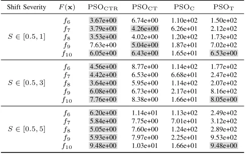
(a)1-dimensional MPB with 3 peaks

(b)1-dimensional MPB with 2 peaks

[image:7.612.51.300.60.142.2]

(c) 2D CMPB with 6 peaks by adding (a) and (b).

Fig. 1. Exponentially growing number of peaks by composing MPBs.

following equations:

h(_it+1)=h_i(t)+αiN(0,1), (8)

w_i(t+1)=w_i(t)+βiN(0,1), (9)

c_i(t+1)=c_i(t)+v(_it+1), (10)

v_i(t+1)= sir

krk, (11)

where N(0,1) is a random number drawn from a Gaussian distribution with mean 0 and variance 1, αi is the height

severity, βi is the width severity,si is the shift severity of the

ith peak, and the components of the vector r are uniformly drawn from[−0.5,0.5]. The reason that each peak has its own width, height, and shift severity is to simulate problems in which different regions change with different intensity. The parameter settings of CMPB are shown in Table I.

An interesting and natural consequence of CMPB’s design is the exponential growth in the total number of peaks as the number of multi-modal components increases. This is a new challenge never addressed in either large-scale global optimization or dynamic optimization. In CMPB, when we compose several MPBs according to (6), the total number of peaks is:

M =

k+l

Y

i=1

mi, (12)

wheremi is the number of peaks in theith MPB subfunction (represented by fi and fj in (6)). It should be noted that

M is the maximum number of peaks that can exist in the landscape, which may change over time due to coverage of smaller peaks by larger ones. For the sake of clarity, we provide an illustrative example. In Fig. 1(a) and Fig. 1(b), two 1-dimensional MPBs with 2 and 3 peaks are shown. The 2-dimensional function constructed based on (6) with

ω1 = ω2 = 1 results in a total of 2 ×3 = 6 peaks. A consequence of this is that even for low-dimensional functions of this form, variable interaction analysis and problem de-composition can significantly simplify the problem. Indeed, an ideal decomposition can reduce the maximum number of peaks down toPk+l

i=1mi which is significantly smaller than (12) for problems with large number of peaks and components. In the next section, we propose a decomposition-based framework that has this feature.

IV. THEPROPOSEDFRAMEWORK

In this section, we propose a cooperative coevolutionary multi-population framework for solving large-scale DOPs. We

first provide an overview of the framework with an emphasis on its high-level structure and the resource allocation policy (Section IV-A). We then focus on the details of our multi-population part of the framework and address dynamic issues such as convergence detection of populations, avoiding mutual convergence of populations onto the same peak, diversity control, and detection and handling of environmental changes (Section IV-B).

A. The high-level structure of the proposed framework

Algorithm 2 shows the structure of the proposed framework. The framework has three major parts – decomposition, search and resource allocation, and change management – which are explained next. In addition to Algorithm 2, Fig. S-1 in the supplementary document illustrates the flow chart of the proposed framework.

1) Decomposition: The framework starts by decomposing a given dynamic optimization problem into its constituent independent components (Algorithm 2, line 1). This is done using a variable interaction analysis algorithm. In this paper, we use the state-of-the-art DG2 algorithm [24] introduced in Section II. After problem decomposition, a multi-population dynamic optimizer is initialized for each of the identified components (Algorithm 2, lines 2-3). It should be noted that each component contains partial solutions which cannot be evaluated directly using the objective function. Due to the black-box nature of the objective function, these partial so-lutions can only be evaluated within the context of a complete solution referred to as acontext vector[28] which is randomly initialized on line 4.

Next, the framework enters its main loop and optimizes the identified lower-dimensional components in an iterative manner (Algorithm 2, lines 5-41). The framework has three major phases: 1) exploration, 2) exploitation, and 3) change management. In the first phase (Algorithm 2, lines 6-23), the framework cycles over all components with the aim of tracking optima, discovering any emerging optima, and estimating the contribution of each component in improving the overall objective function value. For this purpose, the framework maintains a free population and a set of tracker populations for each component. The primary purpose of a free population is to find uncovered peaks. When a free population has converged to a peak, it will change to a tracker population whose primary purpose is to do exploitation and track it after each environmental change. For better use of the limited computational resources between successive environmental changes, the framework detects and deactivates the converged tracker populations based on a mechanism which will be explained in the next section.

(8)

an environmental change, and discrepancy in the convergence behavior of populations.

For best use of the available resources, the exploitation phase occurs at two levels: component level, and population level. At the component level, the best contributing component is selected and all its active tracker populations are executed for an extra iteration (Algorithm 2, lines 24-26). The amount that each component improves the objective value at the end of the exploration phase is taken as its contribution. This often happens for the component experiencing the most intense environmental change. Therefore, by allocating more computational resource to such populations, the algorithm ac-celerates the optimization process by prioritizing components with higher importance or higher change severities. Finally, at the population level, the best tracker of each component is executed for one more iteration (Algorithm 2, lines 27-29). This step not only gives more resources to the best performing tracker, but also keeps the information about the best partial solutions up-to-date for the purpose of updating the context vector.

3) Change Management: Finally, the last phase deals with the environmental changes and updating of the context vector. Two events trigger the updating of the context vector. The first and most obvious case is the detection of an environmental change (Algorithm 2, lines 30-37). The second is prior to the deployment of a solution (Algorithm 2, lines 38-40). In DOPs, the algorithm is given a predefined time frame within which it has to respond to an environmental change. We denote this withηwhich is the maximum number of function evaluations available to the optimizer before providing a solution for deployment. It should be noted that in classic CC, the context vector is updated at every coevolutionary cycle. This is a costly operation because all solutions whose fitness were calculated with a previous version of the context vector have to be re-evaluated. However, owing to the grouping accuracy of DG2 and the independent nature of the components, this operation can be delayed until it becomes necessary (due to a dynamic change).

B. Dynamic Considerations

The aim of the framework on each component is to find all peaks and track them. However, due to the lack of information about the number of peaks, and also the coverage of some smaller peaks by larger ones in some of the environments, a free population needs to constantly search for possible uncovered peaks. Once a new optimum is found by a free population, it changes to a tracker population. To test the convergence of a free population, we use the procedure in which the Euclidean distances between all pairs of individuals are calculated. If all calculated distances are smaller than a given threshold (rconv), it is assumed that the free popula-tion is converged [43]. When a free populapopula-tion becomes a tracker population, a new free population will be initialized immediately in the search space in order to search for another uncovered peak. It is possible that a free population converges to a peak already covered by a tracker population. Tracking a peak by multiple populations wastes a considerable amount

Algorithm 2: The Proposed Framework

1 G=Grouping(f);

2 forallG do

3 Pfree←Initialize the free population;

4 c←Randomly initialize the context vector;

5 repeat

6 forallGdo

7 (Pfree,gfree? ) =Optimizer(Pfree,g?free);

8 ifdiversity of the free population is< rconvthen

9 Change its status to tracker population;

10 Pfree←Initialize a new free population;

11 foreachtracker populationido

12 ifkg?_free−g?_ik< rexclthen

13 Pfree←Reinitialize the free population;

14 ifithtracker population is activethen

15 (Pi,g?i) =Optimizer(Pi,gi?); 16 ifthe diversity is< rdeactthen

17 Deactivate the tracker population;

18 foreachtracker populationsjdo

19 ifkg?_i−g?_jk< rexclthen

20 iff(gi?)< f(g?j)then

21 Removeithtracker population;

22 else iff(g?_i)> f(g_j?)then

23 Removejthtracker population ;

24 Determine the componentHwith the highest progress;

25 forallactive tracker populationsiinHdo

26 (Pi,g?i) =Optimizer(Pi,gi?); 27 foreachGdo

28 Determine the best tracker populationb;

29 (Pb,g?b) =Optimizer(Pb,g?b); 30 ifan environmental change is happenedthen

31 c←Update context vector using best found position in each populationg?_;

32 forallGdo

33 Re-evaluate all individuals of the free population;

34 foralltrackersdo

35 Update estimated shift severity by Eq. (15);

36 Activate if is deactivated;

37 Increase diversity by Eq. (14);

38 ifcomputational budgetηis finishedthen

39 c←Update context vector using best found position in each populationg?;

40 Re-evaluate all individuals in all populations;

41 untilstopping criterion is met;

of computational resource. Therefore, a mutual exclusion principle is enforced to avoid more than one population to cover the same peak. To establish the mutual exclusion, we use the mechanism proposed in [43]. According to the exclusion mechanism, when Euclidean distances between the global best of the free population and a tracker population is less than a threshold (rexcl), the algorithm assumes that the free population has converged to a covered peak. In this situation, the free population will be re-initialized. The value ofrexcl is calculate as follows:

rexcl= 0.5

SR D√

TN, (13)

whereSRis the range of search space andTNis the number of trackers.

(9)

exclusion area of a covered peak. As a result, it becomes a tracker population and moves toward the peak’s center. This is another case where the exclusion principle is enforced to control the computational overhead. To do so, the tracker with the second best found position’s fitness value f(g?₎ _{will be}

removed. For determining tracker populations which are under exclusion condition, the Euclidean distance between all pairs of trackers’ g? _{position is calculated and compared with}_r

excl based on (13).

Another critical challenge of the population-based opti-mization algorithms in DOPs is diversity loss. According to [4], there are two main groups of methods to address this challenge. First is the reaction methods which introduce diversity after each environmental change, and second is diversity maintenance methods which try to keep the diversity of population above a certain level over time.

Our multi-population part of the framework uses a reaction type method in which the trackers’ diversities are increased at the beginning of each environment. When a change is detected, for each tracker, one of the individuals is located on the g?

position from the previous environment and other individuals are randomized around the g? _{position with radius of shift}

severity of the peak by (14):

Pi,j= (si·r) +g

?(t−1),end

i , (14)

where Pi,j is the position of the jth individual of the ith

tracker population andg_i?(t−1),endis its best found position at the end of the previous environment,si is the shift severity of the peak which is under cover of theith tracker population, and r is a uniformly distributed random number vector in range

[−1,1]. The reason for usingsiin (14) is that the new location of the peak after environmental change is expected to be inside that radius from the previous peak center. In (14), theg∗from the end of the previous environment is used instead of previous peak center position. Therefore, the diversity is introduced to the population of each tracker as much as needed. The shift severity of each peak is estimated by (15):

ˆ

si=

1

t−bi−1·

t−1

X

k=bi+1 g

?k,end

i −g

?(k−1),end

i

, (15)

wheresˆi is the estimated shift severity of the peak covered by ith tracker population,bi is the time index of the environment

that ith tracker population has started tracking the peak, t is the current environment time index and g?k,_i endis the global best position of the ith tracker population at the end of the

kth environment.

Another diversity related issue is detection and deactivation of converged trackers to save computational resources. When a tracker population gets sufficiently close to the center of a peak, it should be deactivated until the next environment. A tracker population is deactivated when its diversity drops below a certain threshold. To measure the diversity of a tracker population the infinity norm distance between all pairs of individuals is calculated. If all distances fall below a predefined value (rdeact), the tracker population will be deactivated which means that its individuals freeze until another environmental change is detected. rdeact is a positive constant number. A

TABLE I

PARAMETER SETTINGS OFCMPB

Parameter Symbol Value

Number of peaks m Randomized*between 1 to 10

Dimension D 1-200

Evaluations between changes f 500D

Shift severity s Randomized*∈[0.5,3] Height severity α Randomized*_∈_[3_,_10] Width severity β Randomized*_∈_[0_.₅_,₁_._5]

Peaks shape – Cone

Peaks location range SR [-50,50]

Peak height h [30,70]

Peak width w [1,12]

Initial height value – 50

Initial width value – 6

Number of environments – 100 Weight ω Randomized*_∈_[0_.₅_,_2]

*_{Randomized with uniform distribution.}

positive attribute of using infinity norm distance here is that it is independent from dimension number.

Another challenge of DOPs is outdated memory which happens after each environmental change due to the outdated stored fitness values of positions such as g?. For addressing this issue, after each environmental change, the fitness values of all necessary positions (depends on the component opti-mizer) of the free population will be re-evaluated. For tracker populations, after re-diversification, the fitness values of the necessary positions are evaluated. For example, if PSO is embedded into the framework, the fitness values of particle positions are evaluated and the personal best positions are set to the particle positions.

The final main challenge is change detection. Since de-tecting a change is a separate issue and in most real-world dynamic environments the occurrence of a change is obvious (e.g., arrival of new order, change in temperature) [38], in this paper, we assume that the framework will be informed when an environmental change happens. However, it should be noted that environmental changes can be detected easily in many problems (including the ones that we investigate in this paper) by re-evaluating some beacons [4].

V. EXPERIMENTS ANDANALYSIS

The experiments in this section are based on different scenarios of the CMPB framework described in Section III. Section V-A covers the experimental settings, and Section V-B covers the experimental analysis which contains three sets of experiments. The first set is concerned with investigat-ing the efficacy of decomposition and resource allocation in the proposed framework (Section V-B1), the second set is concerned with investigating the robustness of the proposed framework with respect to various aspects of DOPs, such as the number of peaks, shift severities, and change frequencies (Section V-B2), and the third is to investigate the effect of different component optimizers on the relative performance of the framework (Section V-B3)to demonstrate that the results hold independent of the component optimizer used.

(10)

TABLE II

SUMMERY OF UTILIZED APPROACHES IN THE FRAMEWORKS

Framework Cooperative Tracking multiple Resource coevolutionary moving optima allocation

CTR 3 3 3

CT 3 3 5

C 3 5 5

T 5 3 5

1) Compared Frameworks: To study the effectiveness of different components of the proposed framework, i.e., co-operative coevolution (indexed by C), tracking of moving optima (indexed by T), and resource allocation (indexed by R), we generated four different frameworks which take these components into account in isolation as well as together. These cases are summarized in Table II.

The first framework (T) has no decomposition or resource allocation mechanism and is a representative of the classic TMMO algorithms. For a fair comparison, this framework uses the multi-population approach presented in Section IV-B. The second framework (C) is a simple CC framework which uses DG2 for problem decomposition and uses a single-population optimizer for each component. This framework represents large-scale static methods with no designated mul-tiple optima tracking mechanism. After each environmental change, it simply re-initializes the subpopulations while main-taining the best solution. The third framework (CT) is the combination of the previous two cases, which is identical to our proposed framework (CTR) with the exception of the resource allocation mechanism. CT represents the state-of-the-art GCM-PSO [60] and replicates its major features and unifies its underlying decomposition and the multi-population optima tracking mechanisms for a fair comparison. The last framework (CTR) represents our proposed framework with all three features active.

All the frameworks presented above can be used with any component optimizer. For our empirical analysis, we use four popular component optimizers: PSO [77], jDE [78], [79], DynDE [44], [80], and CMAES [81]. For the experiments in Sections V-B1 and V-B2, we use PSO as the component optimizer due to its popularity in the dynamic optimization literature [4], [37]. The remaining algorithms are used in Section V-B3 to test the effect of different component op-timizers on the proposed frameworks and to show that main conclusions are independent of the component optimizer used.

2) Parameter Settings: The parameter settings of all al-gorithms and frameworks are given in Table III. The right column shows whether the settings are taken from the original reference or from the sensitivity analysis results reported in the supplementary document. The parameters common to all algorithms are also listed at the bottom of the table. For all frameworks, the context vector is updated only after environmental changes and when the computational budget η

is used. The default value ofη isf−1 which means we fetch the solution at the end of each environment.

3) Performance Indicator: To measure the efficiency of algorithms, the average error of the updated context vector at the time of deployment (determined by η) after each

TABLE III

PARAMETERSETTINGS

Alg. Param. Frameworks Ref.

CTR CT T C

CMAES λ 5 30 Tables S-IV, S-VIII

µ bλ/2c [81]

jDE

N P 7 20 Tables S-II, S-VI

Cr self adaptive∈[0,1] [78]

F self adaptive∈[0.1,0.9] [78] strategy DE/rand/1/bin [78]

DynDE

N P 10 60 Tables S-III, S-VII Brownian 3 Tables S-III, S-VII

F, Cr random uniform∈[0,1] [80]

strategy DE/best/2/bin [80]

PSO

C1=C2 2.05 [82]

χ 0.729843788 [82]

5 ford≤5 50 Tables S-I, S-V swarm size 7 for5< d≤7 50 Tables S-I, S-V 10 ford >10 50 Tables S-I, S-V

Common Parameters

rdeact 0.1 – – – Table S-XI

rconv rexcl – [43]

environmental change is used as the measure of performance:

P = 1

T T

X

t=1

f(t)Optimum(t)−f(t)c(t),η, (16)

wherec(t),η_{is the context vector at the}_t_{th environment which}

is updated afterηfitness evaluations since the beginning of the new environment.

B. Empirical Analysis

To compare the performance of the four algorithms, we test them on 20 functions with various characteristics created using the CMPB benchmark generator. The suite contains functions with five different variable interaction structures tested in 25-, 50-, 100-, and 200-dimensional spaces (Table IV). The statistical results are based on 31 independent runs and their median are reported for comparison (mean and standard error are reported in the supplementary document). To test the statistical significance, we perform a multiple comparison test based on a series of pairwise Wilcoxon signed-rank tests with Holm-Bonferroni p-value correction with α = 0.05. Highlighted entries are not statistically different from the best result.

[image:10.612.75.273.84.145.2]

(11)

TABLE IV

BENCHMARKSCENARIOSBASED ONCMPB.

F D Dimensionality of Nonseparable Components Separable

f1 25 {2,4,6,8} 5

f2 25 {2,5} 18

f3 25 {2,4,5,6,8} 0

f4 25 — 25

f5 25 {25} 0

f6 50 {2,3,5,6,7,8,10} 10

f7 50 {2,3,5,5} 35

f8 50 {2,2,3,5,5,5,5,5,8,10} 0

f9 50 — 50

f10 50 {50} 0

f11100 {2,2,3,5,5,6,6,8,8,10,10,15} 20

f12100 {2,2,3,3,5,5,10} 70

f13100 {2,2,2,2,3,3,5,5,5,5,5,5,8,8,10,10,20} 0

f14100 — 100

f15100 {100} 0

f16200 {2,2,3,5,5,6,6,8,8,10,10,15,20,20,30} 50

f17200 {2,3,5,10,20,30} 130

f18200 {2,2,2,3,5,5,5,5,5,8,8,10,10,10,20,20,30,50} 0

f19200 — 200

f20200 {200} 0

TABLE V

COMPARATIVE RESULTS OFPSOCTR,PSOCT,PSOC,ANDPSOTON

f1TOf20. THE HIGHLIGHTED ENTRIES ARE SIGNIFICANTLY BETTER USING PAIR-WISEWILCOXON SIGNED-RANK TEST WITHHOLMp-VALUE

ADJUSTMENT(α= 0.05).

Dim Function PSOCTR PSOCT PSOC PSOT

25D

f1 2.35e+00 3.95e+00 5.93e+01 6.43e+01

f2 2.23e+00 3.24e+00 3.17e+01 9.55e+01 f3 1.19e+00 2.87e+00 5.71e+01 4.30e+01 f4 3.00e+00 3.19e+00 1.10e+01 3.21e+02

f5 1.84e+00 2.94e+00 1.38e+01 1.24e+00

50D

f6 4.56e+00 8.77e+00 1.14e+02 1.77e+02

f7 4.42e+00 6.53e+00 6.68e+01 2.47e+02 f8 3.64e+00 5.95e+00 1.14e+02 2.07e+02 f9 6.08e+00 6.73e+00 2.17e+01 8.16e+02 f10 7.76e+00 8.38e+00 1.66e+01 8.05e+00

100D

f11 1.05e+01 2.02e+01 2.13e+02 6.45e+01

f12 1.19e+01 1.51e+01 1.31e+02 5.71e+02

200D

f16 3.63e+01 5.19e+01 3.39e+02 9.78e+02

f17 3.77e+01 5.60e+01 2.92e+02 5.79e+02

reasons can be attributed to the poor performance of PSOT on majority of the functions. First is the scalability issue. It is clear that in the absence of problem decomposition, the dimensionality of a given problem can easily exceed the capacity of the optimizer. Second, is the exponential growth in the number of peaks when no decomposition is used (see Fig. 1).

In addition to problem decomposition, resource allocation is another major feature ofPSOCTR. The effectiveness of the resource allocation mechanism can be checked by comparing it withPSOCT whose only difference lies within its resource allocation policy. Table V clearly shows the superiority of

PSOCTR over PSOCT. Although problem decomposition plays a crucial role in simplifying a large-scale problem,

TABLE VI

OBTAINED RESULTS BY ALGORITHMS ONf6TOf10WITH DIFFERENT

NUMBER OF PEAKSmFOR EACH COMPONENT RANDOMIZED IN THE

FOLLOWING RANGES{1, . . . ,5},{1, . . . ,10},AND{1, . . . ,20}. OTHER

PARAMETERS OFCMPBARE SET AS SHOWN INTABLEI.

# Peaks F(x) PSOCTR PSOCT PSOC PSOT

m∈ {1, . . . ,5}

f10 6.17e+00 8.08e+00 1.45e+01 7.75e+00

m∈ {1, . . . ,10}

f6 4.56e+00 8.77e+00 1.14e+02 1.77e+02

f10 7.76e+00 8.38e+00 1.66e+01 8.05e+00

m∈ {1, . . . ,20}

f6 9.52e+00 1.33e+01 1.12e+02 2.02e+02

the existence of numerous components can impose a com-putational overhead on the algorithm. Additionally, use of a multi-population algorithm to optimize the components also adds to the computational complexity. The component-level and population-level resource allocation policies ofPSOCTR allow for an economical use of resources while preserving the simplifying effects of problem decomposition. The population-level mechanism prevents over-exploitation of trackers and releases more resources to be used by the best trackers to improve the overall solution quality. The component-level mechanism accelerates the convergence by allocating more resources to the component with maximum impact on the overall solution quality. On the fully nonseparable functions however (f5, f10, f15, and f20), the only active resources allocation mechanism is the population level. The relative high dimensionality of the only available component causes the population-level mechanism to lose its efficiency because of slow convergence and existence of many active populations.

Another interesting observation is a sharp contrast between the performance of multi-population methods (PSOCTR and

PSOCT) and the only single-population method (PSOC). These are all decomposition based where each component is optimized independently.PSOCTR andPSOCT use multiple populations for each component whereasPSOC uses a single population for each component. All these methods benefit from an ideal decomposition which eliminates the issue of expo-nentially growing number of peaks. However, the comparison clearly shows that a special mechanism for tracking multiple moving optima should be in place to obtain acceptable results. In other words, simple mechanisms such re-initialization and injection of the best found solution into the population are not sufficient for efficient handling of environmental changes.

(12)

0 0.5 1 1.5 2 2.5 3 3.5 4 4.5 5 105 100

101 102 103 104

PSO

CTR PSOCT PSOC PSOT

(a) Convergence plot forf6

0 0.5 1 1.5 2 2.5 3 3.5 4 4.5 5

105 100

101 102 103 104

PSO

CTR PSOCT PSOC PSOT

[image:12.612.316.559.120.274.2]

(b) Convergence plot forf7

Fig. 2. Convergence plot ofPSOCTR,PSOCT,PSOCandPSOTbased on the average current error of 31 runs onf6andf7for the first 20 environments.

change.PSOCTRandPSOCTwhich are decomposition-based and track multiple optima outperformPSOTandPSOCacross all environments.PSOCTRhas a clear advantage overPSOCT due to its efficient resource allocation mechanism. As can be seen in Fig. 2, for the first environment, algorithms try to find uncovered peaks to track them after environmental changes. That is why the results obtained in the first environment are worse. This circumstance is more obvious for PSOCTR and PSOCT which suffer from uncovered peaks until the fifth environment. After this phase, the algorithms are more stable and their results are improved because most peaks are identified and the trackers can converge faster to the new optimum after each environmental change.

2) Robustness to Dynamic Changes: Table VI shows the results obtained by the four algorithms onf6-f10with different number of peaks1. The results show that the performance of all algorithms deteriorates as the number of peaks increases. How-ever,PSOCTRmaintains the best performance across all three cases. For the multi-population algorithms (PSOCTR,PSOCT, and PSOT) the increase in the number of peaks results in more tracker populations, which increases the computational overhead of these algorithms. Among these methods, PSOT has the worst performance and experiences an exponential growth in the number of peaks due to its lack of decomposition (see Fig. 1). PSOCTR performs better than PSOCT thanks to its resource allocation mechanism, which makes it less susceptible to an increase in the number of peaks (hence more trackers). PSOC, which maintains a single population, also suffers from an increase in the number of peaks. The reason is that the increased number of peaks adds to the complexity of the landscape and increasing the likelihood of a premature convergence.

Table VII shows the obtained results by the four algo-rithms on f6-f10 with different shift severities1. It is clear that stronger shift severities, i.e., larger displacement in the

TABLE VII

OBTAINED RESULTS BYPSOCTR,PSOCT,PSOC,ANDPSOTONf6

TOf10WITH DIFFERENT SHIFT SEVERITY VALUES FOR EACH PEAK IN

EACH COMPONENT. THE VALUES ARE RANDOMIZED IN THE FOLLOWING

RANGES[0.5,1],[0.5,3],AND[0.5,5]. OTHER PARAMETERS OFCMPB

ARE SET AS SHOWN INTABLEI.

Shift Severity F(x) PSOCTR PSOCT PSOC PSOT

S∈[0.5,1]

f6 3.67e+00 6.74e+00 1.10e+02 1.50e+02 f7 3.79e+00 4.26e+00 6.26e+01 2.12e+02

f8 3.53e+00 4.02e+00 1.20e+02 1.73e+02

f9 7.63e+00 5.04e+00 1.87e+01 7.02e+02 f10 6.05e+00 6.43e+00 1.65e+01 6.53e+00

S∈[0.5,3]

f6 4.56e+00 8.77e+00 1.14e+02 1.77e+02 f7 4.42e+00 6.53e+00 6.68e+01 2.47e+02

f8 3.64e+00 5.95e+00 1.14e+02 2.07e+02

f9 6.08e+00 6.73e+00 2.17e+01 8.16e+02 f10 7.76e+00 8.38e+00 1.66e+01 8.05e+00

S∈[0.5,5]

f9 5.93e+00 7.97e+00 2.25e+01 9.53e+02

f10 9.48e+00 1.03e+01 1.66e+01 9.48e+00

TABLE VIII

OBTAINED RESULTS BYPSOCTR,PSOCT,PSOC,ANDPSOTONf6

TOf10WITH DIFFERENT CHANGE FREQUENCIES:200D,500D,AND

1000D. OTHER PARAMETERS OFCMPBARE SET AS SHOWN INTABLEI.

Frequency F(x) PSOCTR PSOCT PSOC PSOT

f= 200D

f6 1.83e+01 2.90e+01 1.93e+02 2.76e+02

f10 1.20e+01 1.51e+01 1.97e+01 1.36e+01

f= 500D

f6 4.56e+00 8.77e+00 1.14e+02 1.77e+02

f= 1000D

f6 1.90e+00 2.84e+00 9.08e+01 1.62e+02

f7 2.16e+00 1.91e+00 4.55e+01 2.30e+02

location of a peak, makes tracking more difficult and time consuming. Table VII shows thatPSOCTRhas the best overall performance across all three severity levels. The results clearly show that PSOCTR has a better competitive advantage on problems with stronger shift severities. The resource allocation mechanism of PSOCTR allows it to prioritize its limited computational resources for tracking of important peaks. On simpler problems with a smaller shift magnitude, other algo-rithms with no resource allocation mechanism such PSOCT can also track the peaks with a relatively good efficiency and accuracy. This is because the amount of available function evaluations between successive environmental changes is large enough to track all the peaks accurately.

(13)

to degraded performance. Despite this, a desired property of

PSOCTR is its good performance on problems with a high change frequency. The results clearly show that thePSOCTR gains a significant competitive edge over other algorithms on such problems. This can be attributed to its resource allocation mechanism which allows it to benefit from the saved resources to respond to rapid environmental changes more efficiently. This property is less crucial for problems with low change frequencies, due to the availability of sufficient time between environmental changes for accurate tracking of all the peaks.

3) The Effect of Component Optimizers: In this part, we investigate the influence of several component optimizers on the performance of the proposed framework. We compare the performance of the frameworks when PSO [82], jDE [78], [79], DynDE [44], [80], and CMAES [81], [83] are used as the optimizer. For all multi-population algorithms, we use the same mechanism described in Section IV-B.The reason is that our aim here is to confirm that our conclusions are independent of the component optimizer used, not the effect of different dynamic handling mechanisms.

The core procedure of CMAES [81] is very different from PSO and DE. Therefore, for embedding it in the frameworks, we need to carry out some modifications. Instead of the best found position, the mean position is used. For calculating the diversity of each population in CMAESCTR,CMAESCT and CMAEST, we calculate the Euclidean distance between all pairs of offspring (i.e., prior to selection). After each environmental change, the mean positions of all free and tracker populations are re-evaluated. Moreover, for the free population, all other state variables remain unchanged. For trackers however, all state variables relating to the covariance matrix and the evolution path are reinitialized since the direc-tions towards the new optima are unknown. For theith tracker, the step-size (σi) is set to si/ˆ 2 where ˆsi is the estimated shift severity of its covered peak. The reason for choosing

ˆ

si/2 for σi is that the offspring are normally distributed and approximately 95.4% of them are located within 2 standard deviations from the mean. This makes the diversity of new samples in CMAES similar to those of PSO and DE trackers after re-diversification by (14).

Table IX shows the results obtained by the four frameworks using PSO, CMAES, jDE and DynDE as component optimiz-ers on f6-f10 (see Table IV). The results clearly show that our proposed framework (CTR) consistently outperforms other cases independent of the chosen optimizer. Additionally, com-paring the component optimizers across different frameworks shows that PSO has the best performance with CTR; however, comparing the efficacy of component optimizers is beyond the scope of this study.More comparative results obtained by the four frameworks from Table II with the above mentioned component optimizers on different 100 and 200-dimensional problems with different dynamic configurations of CMPB, can be found in Section S-V of the supplementary document.

1_{Other parameters of CMPB are set based on Table I.}

TABLE IX

OBTAINED RESULTS BY THE FOUR FRAMEWORKS FROMTABLEIIWITH

DIFFERENT OPTIMIZERS INCLUDINGPSO,JDE, DYNDE,ANDCMAES

ONf6TOf10WITH DEFAULT PARAMETER SETTING OFCMPB (TABLEI).

Framework

Optimizer F CTR CT C T

PSO

f9 6.08e+00 6.73e+00 2.17e+01 8.16e+02

f10 7.76e+00 8.38e+00 1.66e+01 8.05e+00

CMA-ES

f10 1.11e+00 1.33e+00 1.08e+01 5.90e+02

DynDE

f10 4.53e+00 4.92e+00 1.26e+01 5.20e+00

jDE

f6 2.11e+01 3.43e+01 7.80e+01 1.19e+02

VI. CONCLUSION

In this paper, we presented a thorough investigation of large-scale dynamic optimization problems (DOPs). A formal analysis of the moving peaks benchmark (MPB) showed that its lack of modularity limits its applicability to the study of large-scale DOPs. A new benchmark generator based on MPB was proposed for large-scale DOPs. The benchmark was made by composing several weighted MPBs in which an automated weight regulates the equilibrium between fully separable and nonseparable components, and a manual weight creates artificial imbalance among the contributions of differ-ent compondiffer-ents.

We also proposed a cooperative coevolutionary multi-population framework which benefits from a bi-level com-putational resource allocation mechanism capable of saving resources at both component and sub-population levels. We in-vestigated the performance of the proposed framework against three other frameworks on a wide range of problems having different dimensions, interaction structures, shift severities, number of peaks, and change frequencies.The results showed that the proposed framework not only outperforms the peer frameworks, but also gains even a greater competitive advan-tage on more difficult problems with higher dimensionality, number of peaks, change frequency or shift severity.