Contents lists available atScienceDirect
Computational Statistics and Data Analysis
journal homepage:www.elsevier.com/locate/csda
Hierarchical model for forecasting the outcomes of binary
referenda
Arkadiusz Wiśniowski
a,*
, Jakub Bijak
b, Jonathan J. Forster
b,c,
Peter W.F. Smith
baSocial Statistics Department, University of Manchester, United Kingdom bESRC Centre for Population Change, University of Southampton, United Kingdom cSchool of Mathematics, University of Southampton, United Kingdom
a r t i c l e i n f o
Article history:
Received 14 December 2017 Received in revised form 13 September 2018
Accepted 17 September 2018 Available online 27 September 2018
Keywords: Opinion polls Forecasting Bayesian inference Statistical modelling United kingdom Brexit
a b s t r a c t
A Bayesian hierarchical model is proposed to forecast outcomes of binary referenda based on opinion poll data acquired over a period of time. It is demonstrated how the model provides a consistent probabilistic prediction of the final outcomes over the preceding months, effectively smoothing the volatility exhibited by individual polls. The method is illustrated using opinion poll data published before the Scottish independence referendum in 2014, in which Scotland voted to remain a part of the United Kingdom, and subsequently validate it on the data related to the 2016 referendum on the continuing membership of the United Kingdom in the European Union.
©2018 The Authors. Published by Elsevier B.V. This is an open access article under the CC BY license (http://creativecommons.org/licenses/by/4.0/).
1. Introduction
Opinion polls provide predictions of the outcomes of voting events such as elections or referenda, based on samples drawn from the population that is eligible to vote. Forecasting from opinion polls can be of widespread interest: to the public, to the media, to those running campaigns, or to individuals standing for election. The forecasts can also aid decision making, for example on the amount of money spent on campaigning, by providing a description of uncertainty about the outcome of the voting event.
In this article, we propose a method for predicting the outcome of two referenda recently held in the United Kingdom. The first one is the Scottish independence referendum, held on 18 September 2014, and the second one is the referendum on UK’s membership in the European Union (EU) that took place on 23 June 2016. We use a Bayesian hierarchical model to capture the dynamics of the opinion polls. Share of the votes in the polls is assumed to be sampled from a multinomial distribution with overdispersion and a possibility of polling company bias. Next, logit-transformed probabilities of voting for Yes, No and those Undecided are assumed to follow a stationary Ornstein–Uhlenbeck process. We provide a framework that can be subsequently generalised to forecast voting outcomes on the polling day where there are more than two options, such as parliamentary elections with several parties, or to forecast turnout as well as the outcome.
The paper is structured as follows. In Section2, we review the literature on opinion poll forecasting, and provide a general background for both Scottish independence and EU membership referenda. Section3contains a description of the opinion polls data used for making predictions of referendum outcomes. In Section4we present the forecasting model. The results are
*
Correspondence to: Social Statistics Department, University of Manchester, M13 9PL, Manchester, United Kingdom. E-mail address:[email protected](A. Wiśniowski).https://doi.org/10.1016/j.csda.2018.09.007
described and analysed in Section5, with detailed outcomes presented for the Scottish referendum, and the EU membership referendum used for external model validation. In the Section6we conclude and suggest issues for further research.
2. Background
2.1. Forecasting from opinion polls
Forecasting the result of voting events has long been of great interest in democratic countries. The most prominent examples in the statistical literature describe methods for predicting the share of votes for political parties and presidential candidates in national elections, based on pre-election opinion polls (Campbell, 1992;Jackman, 2005, 2009; Lock and Gelman, 2010;Silver, 2012;Linzer, 2013). There are also models for forecasting the outcome of an election, such as a UK general election, based on exit polls (Brown et al., 1999;Curtice and Firth, 2008). These models have been successful in predicting the outcome before the final result is declared. The earlier the polls take place before the event, the less precise they are, as opinion changes over time (e.g.,Campbell and Wink, 1990;Gelman and King, 1993;Campbell, 1996). Nevertheless, they can be useful in identifying trends in preferences of the electorate.
In many models used to forecast US national election outcomes, covariate information, called ‘fundamentals’, is used to create initial forecasts. These, in turn, are used as prior input into a binomial model (Campbell, 1992;Lock and Gelman, 2010;Linzer, 2013). Fundamentals are based on theories of retrospective voting, according to which voters tend to punish current authorities for economic or social crises (e.g.,Kinder and Kiewiet, 1981;Nadeau and Lewis-Beck, 2001;Duch and Stevenson, 2008, citations afterLinzer, 2013). Hence, such fundamentals include economic growth, unemployment rate and geographical variation (e.g.,Campbell, 1992;Linzer, 2013).
Campbell(1992) predicted the outcome of a presidential election for each state in the US. He applies a linear regression with 16 covariates measured at national, regional and state levels, which include, amongst others, macroeconomic variables, opinion polls from early campaign, state’s voting record in the previous two elections, incumbency of a candidate and measures of partisan shifts over time. The assumption of using linear regression to predict an outcome bounded between zero and one is justified by the fact that the predicted shares are likely to lie around 0.5 rather than the boundaries.
Lock and Gelman(2010) analysed deviations of opinion on the state level from the nationwide average. A Bayesian model used for forecasting is based on a normal approximation to a binomial outcome. Their method integrates past election data to form prior distributions for each state outcome, and combines them with information from the state-level opinion polls to create posterior distributions of the shares of vote before the election. To account for overdispersion due to survey issues, such as weighting or clustering as well as uncertainty about opinion shifts between the forecast and the election day, the prior for variance includes information from past opinion polls averaged over states.
The model proposed byLinzer(2013) extends theLock and Gelman(2010) approach by explicitly introducing binomial variability and allowing the model to borrow strength not only across states, but also over time. This is achieved by introducing a random walk model, similar to that ofJackman(2005), for national-level and state-level effects. The logit of the share of the votes is the sum of these effects. Again, historical state-level forecasts are used to form a prior distribution for the state-level effects.
In the models described above, the historic data on actual elections can be utilised for forecasting the outcome of pres-idential or parliamentary elections, as well as assessing the performance of the opinion polls in predicting their outcomes. The 2014 Scottish referendum had no direct precedent, this being the first time that the choice of full independence had been offered to the Scottish electorate. Therefore, there are no data with which to assess the influence of fundamentals on the opinion of the electorate. Furthermore, within the time frame for analysis, fundamental macroeconomic variables do not vary greatly. We consider that the influence of other factors, such as the position of the UK government and the main opposition party on the independence question (both pro-Union), can be more effectively incorporated in the analysis through expert-based priors.
A Bayesian hierarchical model for the evolution of public opinion over time, based on a series of opinion polls, which does not utilise fundamentals, is the state–space model described byJackman(2005,2009). This model assumes that the result of the poll, denoted byy, is a normal variable with mean that includes ‘true’ intentions and a polling company bias (also called ‘house effects’), and a variance approximated from the central limit theorem asy(1
−
y)/
nwherenis a sample size, as inLock and Gelman(2010). This model, however, does not allow for overdispersion. Polls are pooled over time assuming random walk models for the true intentions. The polling company bias is estimated by assuming that the trajectory converges to the known result of the vote on the day of the election.An alternative approach ofBunker and Bauchowitz(2016) is based on a two-stage model. In the first stage, the polls results are aggregated using weighting procedures that account for accuracy of the pollster, margin of error resulting from the size of the poll and timing of the poll. In the second stage, the variability of the voting preferences is taken into account by using a multinomial distribution with a conjugate Dirichlet prior.
There are also a number of articles in the literature that provide models for forecasting the outcome of the voting event on the British general election night (Brown et al., 1999;Curtice and Firth, 2008). These models are useful to predict the outcome right before the event taking place or before the final result has been published. In general, they estimate the deviations of votes from the known outcome of the previous election.
(2005) andLock and Gelman(2010). We model the variability of the polls over time by using a stationary Ornstein–Uhlenbeck process, which accounts for the fact that polls were infrequent in the early stage of the campaign but very frequent close to the referendum day. FollowingLock and Gelman(2010), we also explicitly allow for overdispersion due to the survey issues and the fact that variability between polls is not simply a function of the underlying time-varying proportions. Finally, in our forecasts we assume that the outcome of election remains unknown to the forecasters.
2.2. The Scottish referendum of 2014
Scotland and England have had a shared sovereign since James VI and the Union of the Crowns of 1603. However, after the Acts of Union of 1707 the Scottish Parliament has been incorporated into the Parliament of the Kingdom of Great Britain, with its seat in Westminster, effectively ending the era of independence of both countries. In modern times, the question of self-rule and possible independence of Scotland has returned to the political agenda over 250 years later, mainly since the 1970s, when the referendum on establishing a separate Scottish Parliament first took place on 1 March 1979. Although 52% of voters were in favour, it did not meet the special condition outlined in the Scotland Act 1978 that 40% of the entire electorate have to vote in favour (BBC, 1997a).
As a result of the referendum on 11 September 1997, in 1999 Scottish Parliament (Holyrood) was convened by the Scotland Act 1998 (BBC, 1997b;Scottish Parliament, 2014a). The Scottish Parliament has the power to make laws in so-called Devolved Matters, such as education, justice or health. The Reserved Matters are outside the competence of the Scottish Parliament and remain with the UK Parliament in Westminster. They include, amongst others, defence, foreign policy, energy, and immigration (Scottish Parliament, 2014b).
The independence referendum that took place on 18 September 2014 was enabled by the Scottish Independence Refer-endum Act 2013 (Scottish Parliament, 2013). It asked residents of Scotland a question: ‘Should Scotland be an independent country?’ If the majority of respondents had answered positively, Scotland, according to the Scottish Government White PaperScotland’s Future(Scottish Government, 2013), would have been able to decide about all Reserved Matters, with the monarch of the UK remaining the head of state.
The motivation for developing a model to forecast the outcome of the referendum arose from research on future Scottish migration. As mentioned above, migration policy implemented in Scotland is currently that of the entire UK (McCollum et al., 2014). Forecasts of Scottish migration, prepared before the referendum, had to take into account the uncertainty of the referendum outcome (Wiśniowski et al., 2014). This was achieved by incorporating the probability that Scotland will vote ‘Yes’ in the forecasting framework. This probability was used for averaging the forecasts of Scottish migration under two scenarios: independence andstatus quo. The model developed in the current paper was designed to provide this probability for particular dates prior to the referendum.
2.3. The UK membership in the EU referendum of 2016
On 1 January 1973, the UK has joined the European Communities (in 1992 transformed into the European Union; see e.g. Church and Phinnemore, 1995). This was confirmed by the 1975 European Communities referendum which saw 65% turnout and 67% voters supporting the membership (BBC, 1975). The 2016 referendum on the continuation of the membership in the European Union (EU) was called by the then Prime Minister David Cameron, amidst the rounds of renegotiating the conditions of UK’s future EU membership (UK Parliament, 2016;Nugent, 2017).
The referendum took place on 23 June 2016 and, despite the opinion polls suggesting the outcome in favour of the Remain camp (e.g.BBC, 2016), 51.9% of those eligible voted to leave the EU, with turnout just above 72% (Electoral Commission, 2016). The inconsistency of the polls with the final outcome spurred a discussion on the reasons for discrepancies between the opinion polls and the outcomes of voting events, similar to the one after the 2015 general election (Sturgis et al., 2016). The opinion polls data for the EU membership referendum are used to estimate the probability of the ‘‘Leave’’ outcome and validate the model developed for forecasting the Scottish referendum.
3. Data
3.1. Scottish independence opinion polls data
The data on opinion polls for forecasting Scottish referendum were obtained from the UK Polling Report website1 for each of the ten polling companies. These companies apply various methodologies for polling: YouGov—online polling from a recruited panel of respondents; Survation—online interviews, telephone and face-to-face; TNS-BMRB—face-to-face computer assisted interviews at respondents’ homes; ICM—online polling with stratification by demographic characteristics; Ipsos-Mori—computer-assisted telephone interviews with quota sampling; Panelbase—online polling; Progressive—online polling and telephone interviews; Angus Reid—online polling; Ashcroft—documentation unclear but apparently face-to-face interviews, which seem to have been subcontracted to different companies; and Opinium—online interviews.2 The first
Fig. 1. Opinion polls results by polling company. Available at:http://ukpollingreport.co.uk/scottish-independence-referendum(accessed last on 22 September 2014).
observation comes from 29 January 2012, the last polls were carried out on the eve of the referendum, on 17 September 2014. Categories of voters ‘undecided’ and ‘not voting’ have been merged together into one called ‘Undecided’, though the category of those ‘not voting’ was used in very few polls. Proportional corrections to the Undecided were made if the shares of votes did not sum to one. In the upper plot ofFig. 1we present the percentage of respondents to the opinion poll who declared an intention to vote in favour of independence, out of the total number of those expressing intention to vote. The lower plot shows the percentage of respondents who were classified as ‘Undecided’ at the time of each poll.
3.2. EU membership opinion polls data
The data on opinion polls for the EU membership referendum were obtained from the same source as above,3 and are presented inFig. 2for each of the ten polling companies. The last category ‘‘Other’’ contains polls from companies that polled only once or twice during the considered period. Here, the first observation comes from 9 September 2010 and the last six polls were collected on the eve of the referendum. For clearer picture of the last days before the referendum, figures in Online Supplementary Material depict the data with the time scale converted into the natural logarithm of the number of days left till the referendum day. Given that the data come from the same source as for the Scottish referendum, the same general remarks and caveats as discussed above hold with respect to their key features, interpretations and limitations.
3.3. Data assessment and assumptions
Throughout the paper, we assume that the main sources of error are the sampling error, variability over time and overdispersion. Possible causes of overdispersion include survey issues such as non-independence of respondents or
Fig. 2.EU membership referendum—opinion polls results by polling company.
differences in methodologies used by the polling companies, as well as other factors contributing to differences in polls carried out on the same day such as measurement error. We also allow for the fact that individual polling companies may exhibit a consistent bias across time, but we assume that the average bias across companies is zero. This strong assumption is a direct consequence of the fact that we did not know the outcome of the referendum at the moment of creating a forecast. If the final result is known, the approach ofJackman(2005) can be used to learn about the polling company biases. Alternatively, if there were relevant data on the historic performance of pre-referendum opinion polls, this assumption could be relaxed.
In general, the polling company bias can stem from sources such as the mode of data collection (Jäckle et al., 2010), item non-response (National Research Council et al., 2013) or type of survey (probability and non-probability surveys, see e.g.Sturgis et al., 2016;Baker et al., 2013), to name a few. For instance, face-to-face interviews may induce social desirability bias and reporting behaviours which do not actually occur. This bias tends to be reduced when using telephone interviews (Presser and Stinson, 1998;DeBell et al., 2018). However, in the current application, we do not have access to such details for most of the used polls as we rely on available aggregate summaries of the data described in previous subsections.
We recognise that the usual polling techniques used for elections may not provide such accurate results for a referendum for which polling companies have no previous experience. The main two problems that may distort the accuracy of the opinion polls are overestimation of turnout and differential response rate (e.g.,McAllister and Studlar, 1991;Lynn and Jowell, 1996;Wells, 2014). The differential response rate between prospective Yes and No voters, which, if present here, might be expected to indicate a reluctance to reveal a preference for Scotland remaining in the UK or UK leaving the EU, can lead to a bias in opinion poll results.
acquiescence response biases which can put the validity of the entire prediction of the outcomes into question (DeBell et al., 2018). In their experimental study,Großer and Schram(2010) find that the turnout depends on the information from the opinion polls and floating (undecided) voters. A decrease in turnout can be expected if polls indicate a landslide victory of one option and vice versa, turnout increases with polls showing decreasing differences between the two options. Further, the floating voters are almost entirely responsible for the turnout boosts. Interestingly, in 2004, the pollster Populus categorised 35 percent of the electorate in the UK as floating voters (The Times, 2004).
4. Model specification
In this section we present the bespoke model for forecasting the referendum outcome based on the opinion poll data. Even though the model was initially designed to fit the data on the Scottish referendum, its generality has been subsequently assessed and confirmed in the context of the referendum on the EU membership.
4.1. Forecasting model
In our application, we consider three categories for voting intentions: Yes (1), No (2) and Undecided (3). Let yi
=
(yi1
,
yi2,
yi3) be a vector containing the number of persons declaring to vote for each category in theith opinion poll taken at timet(i) days before the referendum, by polling companyc(i), with a sample sizeni. For each polli,t(i) takes a value in{
t1, . . . ,
tD}
, representingDdistinct polling occasions, andc(i) takes a value in{
1, . . . ,
10}
, as there are ten polling companies.To simplify, we assume that the results of a poll are published at the same time on a given day. In particular, we assume that
yi
∼
Multinomial(ni,
pi),
(1)wherepi
=
(pi1,
pi2,
pi3) is the corresponding probability vector. Letqi=
(qi1,
qi2) be the logit transformation of the category Yes against No, and of the Yes and No categories jointly against the Undecided,qi1
=
log(
pi1pi2
)
,
qi2=
log(
pi1+
pi2pi3
)
.
(2)The logit transformation in(2)ensures that the estimated probabilitiespi1
,
pi2,
pi3remain bounded by 0 and 1.For qi we make the following assumptions. First, we assume overdispersion resulting from the issues discussed in
Section3.3. Second, we account for the possibility of polling company biases, and introduce parameter
γ
to capture it. Finally, we include a parameterρ
to allow for correlation betweenqi1andqi2. Hence, a hierarchical model forqiis as follows:[
qi1qi2
]
∼
N([
θ
1[
t(i)] +
γ
c(i)1θ
2[
t(i)] +
γ
c(i)2]
,
Σ)
,
(3)whereN(
µ,
Σ) denotes a normal distribution with meanµ
and variance matrixΣ, which we parameterise using marginal precisionsτ
21andτ
22and correlationρ
. In(3),θ
1(t) andθ
2(t) are logits of the corresponding proportions in the general population at a timetdays before the referendum. Such a specification assumes that the only difference between opinion polls on a given daytis due to the polling company biasesγ
=
(γ
c1, γ
c2),
c∈ {
1, . . . ,
10}
. These effects are constrained to have a zero mean and are assumed to follow a univariate normal distribution:γ
ck∼
N(
0
, τ
3−k1)
,
k=
1,
2,
c∈ {
1, . . . ,
10}
.
(4)The zero mean here reflects the assumption, discussed in Section3.3, that the average bias across polling companies is zero. Next, we assume that the underlying logits
θ
k(t) follow independent Ornstein–Uhlenbeck processes. Fork=
1,2, wedefine
θ
k=
(θ
1k, . . . , θ
Dk) as logit-transformed proportions in the general population on the dates of the opinion polls in oursample, so that
θ
jk=
θ
k(tj). Therefore, the model forθ
kisθ
jk∼
N(
α
tj−tj−1k
[
θ
j−1k−
f(tj−1, β
k)]
+
f(tj, β
k),
1
−
α
ktj−tj−1τ
1k)
,
(5)wherej
=
1, . . . ,
Dand 0≤
α
k<
1. Functionf(tj, β
k) is the marginal mean ofqik, for any pollitaken on daytj, and specifiesthe time trend using a vector parameter
β
k. Parameterα
kcontrols the extent of serial correlation. For functionfwe considerconstant, linear, quadratic and cubic trend specifications. For example, for the quadratic trend we have
f(t
, β
k)=
β
k0+
β
k1t+
β
k2t2.
By setting the date of the referendum as the origin of the time variablet(t
=
0), the intercept parameterβ
10is the marginal expected logit of the probability of a Yes outcome in the referendum. The forecasted share of votes in favour of independence,s0, is given by
s0
=
exp
[
θ
1(0)]
where
θ
1(0) is a forecast forward tot=
0. Hence,s0is the key parameter of interest taking into account both the underlying trendβ
10and recent divergences of opinion from this trend.The best fitting trend is selected by using the Deviance Information Criterion (Spiegelhalter et al., 2002). Time trend, autocorrelation and precision parameters are specific to the level of the model hierarchyk, as the odds Yes/No (qi1) and (Yes+No)/Undecided (qi2) can behave in different ways over time. In general, different specifications of the time trendf for both logits are also possible.
4.2. Prior distributions
For the model parameters, we assume the following prior distributions. For the key parameter
β
10, the intercept in the mean model for Yes/No odds in(5), we utilise subjective expert information obtained from the Delphi questionnaire on future migration trends in Scotland (Shang et al., 2014;Wiśniowski et al., 2014). The Delphi survey was carried out in June 2013. Information was provided by eight out of 12 experts, who had been asked to state the probability that Scotland would gain independence. This probability can also be interpreted as a probability that the share of the votes will be larger than 50%. This provides partial prior information about the experts’ uncertainty about the share of the votes which we utilise to construct the prior distribution forβ
10as follows.We assume that the prior distribution is an equally-weighted mixture of normal distributions, constructed for each of the eight experts. Since
β
10represents the logit of the expected share of votes on the referendum day, we assume that the probability of share of votes being larger than 50% provided by expertlisPl
=
P(
log Sl 1
−
Sl>
0)
=
1−
Φ(
−
µ
lσ
l)
,
l=
1, . . . ,
8,
(7)whereΦis the distribution function of a standard normal distribution. HereSlis a random variable representing thelth
expert’s opinion on the share of votes on a referendum day, which we assume to have a logistic-normal distribution with mean
µ
land varianceσ
l2. As full information was not provided by the experts about their uncertainty concerning the shareof the votes, there are 16 unknowns in eight equations(7). Therefore, we assume that each expert’s opinion is equivalent to a poll of sizen. In such a poll, we would havenSl
∼
Binomial(n,
pl). Hence, by applying the delta method we obtainσ
2l
=
Var(
log Sl 1
−
Sl)
≈
Var(Sl)(
1
pl(1
−
pl))
2=
1npl(1
−
pl).
(8)Since this variance is the largest forpl
=
0.
5, we simplify(8)toσ
l2≈
4/
n, forl=
1, . . . ,
8. For our application, we assumethat each expert is equal ton
=
125 respondents in a representative opinion poll, so that a total of eight experts is equivalent to 1000 respondents, which is a typical size for an opinion poll. In the sensitivity analysis below we assess departures from this assumption by consideringn=
1 as well as an approximately uniform prior.For the other elements of the vector
β
kwe use normal distributions centred around zero with very large variances:β
ki∼
N(0,
104),
i,
k=
1,
2.
These priors are extremely diffuse, which in principle allows opinion to exhibit variation in time which is much more rapid than might be considered plausible. However, when we use priors with much smaller variances restricting variation in opinion to a more plausible range, the final results were indistinguishable from those with the diffuse priors, indicating the lack of sensitivity to the precise values of the prior variances.
For
α
kwe assume a uniform distribution on (0,
1), which prevents this parameter taking negative values or exhibitingexplosive behaviour:
α
k∼
U(0,
1),
k=
1,
2.
For precisions
τ
1k,τ
2kandτ
3k, we assumed truncated normal distributions:τ
1k∼
N(
0
,
106)
1(τ
1k≥
0),
k=
1,
2,
τ
2k∼
N(
0
,
106)
1(τ
2k≥
0),
k=
1,
2,
τ
3k∼
N(
0
,
106)
1(τ
3k≥
0),
k=
1,
2,
where1(g) is an indicator function taking one ifgis true, and zero otherwise. Finally, for the correlation parameter
ρ
, we assumeρ
∼
U(−
1,
1).
To select the prior distributions for the precisions including the values of the hyperparameters, we analysed the model with data simulated to resemble opinion polls related to the Scottish referendum. This simulation study demonstrated that the use of diffuse conjugate gamma priors (e.g.Γ(10−3
,
10−3)) for the precision parametersτ
5. Results of forecasting referendum outcomes
5.1. General remarks
Predictive distributions of the referendum result, based on the opinion poll data and expert opinion, were obtained by using OpenBUGS (Lunn et al., 2009) and JAGS with
rjags
R package (Plummer et al., 2003, see code repository in Online Supplementary Material). As discussed in Section 4.1,s0 in(6)in the context of the Scottish referendum is the share of the Yes votes, in favour of independence, on the referendum day, and hence uncertainty about the referendum outcome is represented by the posterior distribution ofs0. The probability of an outcome favouring independence is therefore calculated as the probability mass of the predicted share of the Yes votes larger than 50 percent, i.e.P(s0>
0.
5). Similar operationalisation has been adopted for the EU membership referendum, wheres0relates to the share of the Leave votes, favouring the withdrawal of the UK from the European Union.Below, we first present the history of forecasts for the Scottish independence based on the data one year, and then 200, 100, 30 and seven days before the referendum. Next, we use the data that include the polls carried out within the week prior to the referendum as this was the period when nine additional polls were carried out. The time trend with the lowest DIC is quadratic for all subsets of the polling data. Finally, we apply the model to the EU membership referendum data, in order to externally validate the robustness of the method.
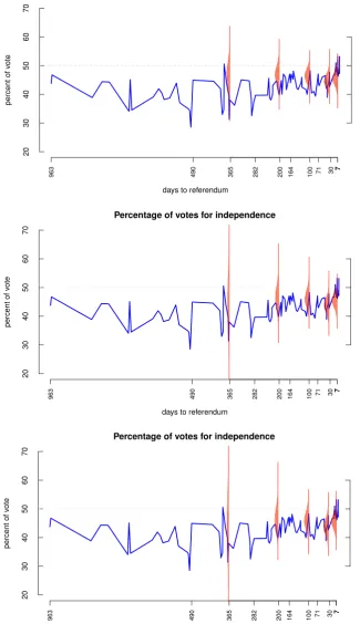
5.2. Scottish referendum: history of forecasts
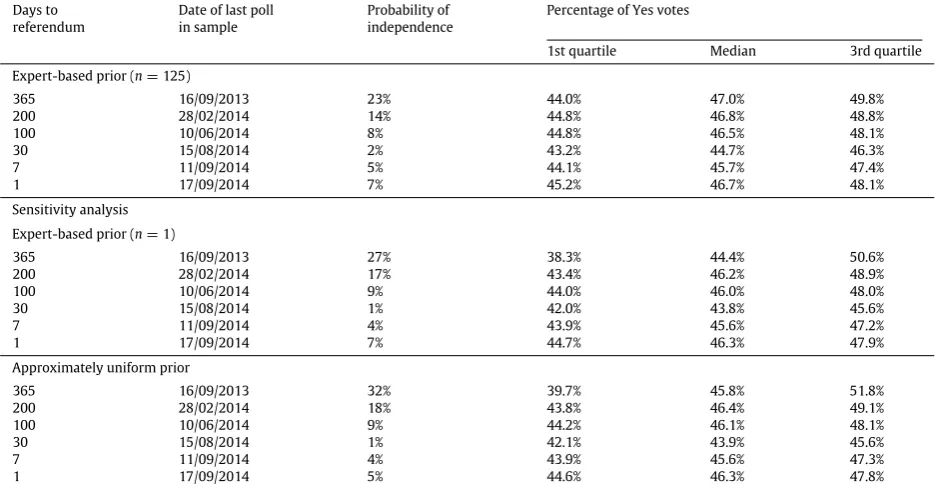
Forecasts of the result of the referendum, together with the opinion poll data until one week before the referendum, are presented in the upper panels ofTable 1andFig. 3. In the last three columns ofTable 1, we present the median and quartiles of the predicted share of Yes votes (excluding Undecided). We observe that the median is almost constant over time, at around 46 percent (with a drop to 44.7 percent one month before the referendum), but the predictive distribution of the share of votes for independence is shrinking with additional observations utilised in the model. An earlier version of our model,4 which did not include the polling company effect
γ
, produced undesirable sensitivity of the forecasts to the order in which different companies published their polls and led to an overestimation of the proportion in favour of independence at certain dates.The results indicate that one year before the referendum, there was still room for a change in the opinion for both Yes and No camps. Closer to the referendum, however, the chances of any dramatic shifts were shrinking. The decrease observed one month before indicates the influence of the debate between the First Minister of Scotland, Alex Salmond, and the leader of the pro-Union campaign, Alistair Darling, on 5 August 2014, deemed to have been lost by the former. Even in the final days of campaigning, the forecasts remained at a similar level, which can be explained by relatively large differences amongst the polls carried out by various companies in the last week. Hence, the uncertainty of the predicted votes share remained rather large, with the interquartile range of 45.2–48.1 percent.
The probability of independence decreased over time from 23 percent one year prior to the referendum, to two percent with 30 days to go (and after the first TV debate on 5 August 2014). The upward shift in the polls conducted a week before the referendum led to an increase of the probability to five percent, which might have been a result of the second TV debate on 25 August, said to have been won by Alex Salmond. The changes in this probability over time are summarised in the upper panel ofTable 1and the corresponding distributions of the share of the Yes vote are presented in the upper panel ofFig. 3.
5.3. Scottish referendum: on-the-eve forecasts
Our final prediction, based on the opinion polls reported up to 17 September 2014, i.e. on the eve of the referendum, is presented in Fig. 4, together with the referendum outcome on 18 September, which was 44.7 percent in favour for independence. This outcome is approximately the 18th percentile of our predictive distribution. Despite the last-minute increase in the probability of independence to seven percent, the median share of Yes votes, 46.7 percent, remained at a similar level to the earlier predictions. The final result also suggests that the opinion polls carried out shortly before the referendum might have been biased towards independence, as they all predicted a higher share of the Yes votes than the final outcome.
The predicted share of the undecided on the day of election was 8.5 percent with the 95% predictive interval being 6.5–10.9 percent. If we assume that all ‘decided’ vote, this provides an estimate of a turnout of 91.5 percent. The actual turnout was at a lower level of 84.6 percent which aligns with the findings about the overestimation of turnout described in Section3.3. Finally, the comparison of the models with quadratic and cubic trends, which in the end were the two competing models, reveals that the differences in the predictions were minimal.
4Presented in the Monkey Cage blog at the Washington Post:Scottish independence vote is too close to call(30 July 2014) andOdds of a Scottish Yes
Table 1
Probability of independence and quartiles of the Yes votes share.
Days to referendum
Date of last poll in sample
Probability of independence
Percentage of Yes votes
1st quartile Median 3rd quartile
Expert-based prior (n=125)
365 16/09/2013 23% 44.0% 47.0% 49.8%
200 28/02/2014 14% 44.8% 46.8% 48.8%
100 10/06/2014 8% 44.8% 46.5% 48.1%
30 15/08/2014 2% 43.2% 44.7% 46.3%
7 11/09/2014 5% 44.1% 45.7% 47.4%
1 17/09/2014 7% 45.2% 46.7% 48.1%
Sensitivity analysis
Expert-based prior (n=1)
365 16/09/2013 27% 38.3% 44.4% 50.6%
200 28/02/2014 17% 43.4% 46.2% 48.9%
100 10/06/2014 9% 44.0% 46.0% 48.0%
30 15/08/2014 1% 42.0% 43.8% 45.6%
7 11/09/2014 4% 43.9% 45.6% 47.2%
1 17/09/2014 7% 44.7% 46.3% 47.9%
Approximately uniform prior
365 16/09/2013 32% 39.7% 45.8% 51.8%
200 28/02/2014 18% 43.8% 46.4% 49.1%
100 10/06/2014 9% 44.2% 46.1% 48.1%
30 15/08/2014 1% 42.1% 43.9% 45.6%
7 11/09/2014 4% 43.9% 45.6% 47.3%
1 17/09/2014 5% 44.6% 46.3% 47.8%
Fig. 4. Probability distribution of the percentage of the votes for independence (red) on the eve of the referendum with the referendum result (black). Shares of votes relate to responses favouring independence and exclude those undecided or not voting. (For interpretation of the references to colour in this figure legend, the reader is referred to the web version of this article.)
5.4. Scottish referendum: sensitivity analysis of the priors
To assess sensitivity of the results to the expert-based prior on
β
10we considered two priors where the expert opinion is moderated. In the first, we reduce the effective weight of each expert ton=
1, and in the second we use a diffuse priorβ
10∼
N(0,
2), which is approximately equivalent to a uniform prior on (0,
1) forE(s0). The results are presented in the second and third panels ofTable 1andFig. 3. As would be expected, the expert-based prior has an influence on the predictive distributions at the earlier polling dates, in 2013 and the spring of 2014, effectively shrinking the predictive distributions. However, there is little sensitivity to the choice of the prior in the run-up to the referendum, as the polling evidence outweighs the earlier expert opinion.5 As a result, the discrepancy between the predicted results close to the referendum day is negligible.5For the on-the-eve prediction, the true referendum outcome is close to the 25th percentile of the predictive distributions obtained by using either the
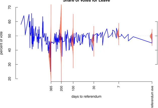
[image:10.544.166.377.363.479.2]Fig. 5. Probability distribution of the share of the votes for Leave on the referendum day (red) with the opinion polls results (blue line). Probability distributions of the share of votes relate to the day of the referendum. They are plotted on the time scale (logged) to denote the moment when the forecast was made. Shares of votes relate to responses favouring withdrawal from the EU and excluding undecided and those not voting. (For interpretation of the references to colour in this figure legend, the reader is referred to the web version of this article.)
5.5. Model validation: EU membership referendum
The EU membership referendum carried out in the United Kingdom in 2016 enabled us to carry out an external validation exercise for the model proposed in Section4. As in this case we did not have access to expert opinion which would be comparable to the information elicited for the Scottish referendum (Section3), the estimation only includes a vague prior distribution for the parameter
β
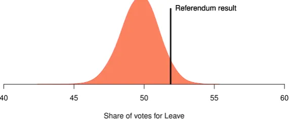
10. As before, the best-fitting trend has been also selected by using the Deviance Information Criterion, with the caveat that forecasts done for different pre-referendum cut-off dates could have been based on different trend functions. In particular, the on-the-eve predictions based on all three trend functions yielded similar predictions as well as approximately the same Deviance Information Criteria.The specific results of the forecasts are presented inFigs. 5–6, as well as inTable 2. Overall, as was the case with the Scottish independence referendum, there is a visible narrowing of predictive intervals over time. Towards the end of the prediction horizon, and especially on the eve of the referendum, the predictions formally remained inconclusive, with the inter-quartile range of the predictive distributions covering 50 percent of the Leave vote. Nevertheless, as seen especially in Table 2andFig. 6, the odds were only slightly for the Leave vote winning. As it happened, the final share of the Leave vote was 51.9 percent. The predicted share of the Undecided vote, a proxy for the share of the electorate that did not vote, was 10.2 percent, with a 95% predictive interval between 7.9 and 13.2 percent. Hence, the model predicted the turnout of 89.8 percent which is again quite well above the actual turnout of 72.2 percent. Here, a likely explanation might be an estimated lower turnout of the young voters aged 18–34 compared to those aged 55–74 (Ipsos-Mori, 2016). A speculative hypothesis for that behaviour might be that, on the day of the referendum, a victory of the Remain camp has been expected as revealed by, e.g., the last published poll which showed 48 to 46 percent for Remain.6 This explanation would align with the findings ofGroßer and Schram(2010). Overall, as in the case of the Scottish referendum, the model performed reasonably well, clearly indicating the uncertainty around the polling outcome.
5.6. Model sensitivity: time trend specification
We analyse the use of cubic B-splines to specify the time functionf(t
, β
k) in(5). This can be viewed as a more generalspecification of the marginal means of the logitqikin(2)that might be useful in the cases where the long-term time pattern
exhibits more erratic behaviour.
In particular, we use two knots that split the data set into three subsets with a similar number of observations in each of them. The indices for the splines are created using function
bs()
from packagesplines
inR(R Core Team, 2018). The results for both Scottish and EU membership referenda are mildly sensitive to the use of the B-splines. For the long-termTable 2
Probability of leaving the EU and quartiles of the Leave vote share.
Days to referendum
Date of last poll in sample
Probability of Leave Percentage of Leave votes
1st quartile Median 3rd quartile
365 24/06/2015 6% 32.0% 36.9% 42.2%
200 06/12/2015 54% 45.0% 50.7% 56.4%
100 15/03/2016 19% 43.8% 46.4% 49.1%
30 24/05/2016 9% 45.5% 46.9% 48.4%
7 16/06/2016 78% 50.2% 51.2% 52.5%
1 22/06/2016 42% 48.9% 49.7% 50.5%
Fig. 6. Probability distribution of the percentage of the votes for Leave (red) on the eve of the referendum with the referendum result (black). The actual outcome is the 95th percentile of the posterior distribution. (For interpretation of the references to colour in this figure legend, the reader is referred to the web version of this article.)
forecasting horizons (100 days before or longer), we observe relatively large uncertainty in predictive posteriors for the vote share under study. These differences diminish for short-term horizons. On the eve of the referendum, the predicted probability of Scottish independence is estimated to be 13 percent compared to 7 percent inTable 1; for the EU membership the corresponding probability of Leave is 43 percent compared to 42 percent inTable 2. The DIC yielded by the models based on B-splines for short-term forecasts are also close to the ones produced by the polynomial trends. Hence, in the cases where no informed judgement can be made about the long-term behaviour of the voting intentions, we recommend Bayesian averaging (Hoeting et al., 1999) of the results to account for the uncertainty about the trend specification for the mean.
6. Discussion
In this paper we have proposed a method of estimating the probability of the outcome of a referendum by using opinion poll data. It takes into account the variation between the polls over time, between the polls carried on the same day, and accounts for the biases of various polling companies. It smooths out the volatility of the opinion polls carried out before the referendum, yet is still able to capture swings in voting intentions. The model can also predict approximate turnout in addition to the outcome of the vote. The method has been applied to the 2014 independence referendum in Scotland and validated on the data for the 2016 UK referendum on continuing membership of the European Union. The actual outcomes of both referenda fall well within the respective predictive probability distributions obtained from our model, and in both cases are close to our predicted median values, with differences of around
±
2 percentage points. [image:12.544.128.414.206.324.2]the model presented in this paper, picking up the second leaders’ debate as the decisive turning point in favour of Scotland remaining in the Union (Wall et al., 2017).
Further research is required for applications such as election forecasting, where additional covariates, such as fundamen-tals or outcomes of historical events, as well as information on past performance of the polls can be utilised. This information could be used for forecasting the spatial distribution of votes, important for the prediction of results for individual electoral districts, for example in the UK parliamentary elections, or the US presidential elections. It could be also used to strengthen the predictions of turnout, which in the current version is biased compared with the actual outcome but is only based on the share of Undecided (i.e. floating) voters whose decisions about turning out are difficult to predict until the actual voting event (Großer and Schram, 2010). Further, the bias across polling companies could be addressed by utilising, if available, information on the mode of data collection, non-response or type of the survey. This information can be incorporated in our modelling framework by including, for example, a generalised linear model for parameters
γ
in(4); alternatively, informative priors reflecting potential biases can be constructed based on expert assessment of the polls. Another extension could be to perform Bayesian model averaging to account for the uncertainty about the particular time trend used to make the prediction. Finally, the time trend could be replaced by other semi- or non-parametric function, such as a normal kernel or other types of splines. Still, after necessary modifications –mainly extending the two-level model hierarchy to more levels –the proposed framework can be easily generalised to forecast voting outcomes with more than two options.Acknowledgements
The Economic and Social Research Council Centre for Population Change (RES-625-28-0001) and Future of Scotland Project are gratefully acknowledged. The authors would like to thank Allan Findlay and David McCollum, and two anonymous reviewers for helpful comments on the earlier draft. All the interpretations in this paper are ours.
Appendix A. Supplementary material
Supplementary material related to this article can be found online athttps://doi.org/10.1016/j.csda.2018.09.007.
References
Auld, T., Linton, O., 2018. The behaviour of betting and currency markets on the night of the EU referendum. In: Cemmap Working Paper CWP 01/18. Institute for Fiscal Studies, London, Available athttps://www.ifs.org.uk/uploads/CWP011818.pdf. (Accessed 20 July 2018).
Baker, R., Brick, J.M., Bates, N.A., Battaglia, M., Couper, M.P., Dever, J.A., Gile, K.J., Tourangeau, R., 2013. Summary report of the AAPOR task force on non-probability sampling. J. Surv. Stat. Methodol. 1 (2), 90–143.
BBC, 1975. 1975: UK Embraces Europe in Referendum. British Broadcasting Corporation, Online material, Available at:http://news.bbc.co.uk/onthisday/ hi/dates/stories/june/6/newsid_2499000/2499297.stm. (Accessed 08 September 2017).
BBC, 1997a. Scottish Devolution. Briefing by Brian Taylor, Political Editor, BBC Scotland. British Broadcasting Corporation, Online material, Available at:
http://www.bbc.co.uk/news/special/politics97/devolution/scotland/briefing/scotbrief1.shtml. (Accessed 12 February 2014).
BBC, 1997b. Scottish Referendum Live –The Results. British Broadcasting Corporation, Online material, Available at:http://www.bbc.co.uk/news/special/ politics97/devolution/scotland/live/index.shtml. (Accessed 12 February 2014).
BBC, 2016. EU Referendum: Did the Polls All Get It Wrong Again? British Broadcasting Corporation, Online material, Available at:http://www.bbc.co.uk/ news/uk-politics-eu-referendum-36648769. (Accessed 08 September 2017).
Brown, P.J., Firth, D., Payne, C.D., 1999. Forecasting on British election night 1997. J. R. Stat. Soc. Ser. A 162 (2), 211–226.
Bunker, K., Bauchowitz, S., 2016. Electoral forecasting and public opinion tracking in Latin America: An application to Chile. Política 54 (2), 207–233. Campbell, J.E., 1992. Forecasting the presidential vote in the states. Am. J. Political Sci. 36, 386–407.
Campbell, J.E., 1996. Polls and votes the trial-heat presidential election forecasting model, certainty, and political campaigns. Am. Politics Res. 24 (4), 408–433.
Campbell, J.E., Wink, K.A., 1990. Trial-heat forecasts of the presidential vote. Am. Politics Res. 18 (3), 251–269.
Church, C.H., Phinnemore, D., 1995. European Union and European Community: A Handbook and Commentary on the 1992 Maastricht Treaties. Prentice Hall, London.
Curtice, J., Firth, D., 2008. Exit polling in a cold climate: The BBC–ITV experience in Britain in 2005. J. R. Stat. Soc. Ser. A 171 (3), 509–539.
DeBell, M., Krosnick, J.A., Gera, K., Yeager, D.S., McDonald, M.P., 2018. The turnout gap in surveys: Explanations and solutions. Sociol. Methods Res. 0049124118769085.
Duch, R.M., Stevenson, R.T., 2008. The economic vote: How political and economic institutions condition election results. Political Economy of Institutions and Decisions. Cambridge University Press, New York.
Electoral Commission, 2016. EU referendum results. Online material, Available at:http://www.electoralcommission.org.uk/find-information-by-subject/ elections-and-referendums/past-elections-and-referendums/eu-referendum/electorate-and-count-information. (Accessed 06 November 2017).
Gelman, A., 2006. Prior distributions for variance parameters in hierarchical models (comment on article by Browne and Draper). Bayesian Anal. 1 (3), 515–534.
Gelman, A., King, G., 1993. Why are American presidential election campaign polls so variable when votes are so predictable? Br. J. Political Sci. 23 (04), 409–451.
Großer, J., Schram, A., 2010. Public opinion polls, voter turnout, and welfare: An experimental study. Am. J. Political Sci. 54 (3), 700–717. Hoeting, J.A., Madigan, D., Raftery, A.E., Volinsky, C.T., 1999. Bayesian model averaging: A tutorial. Statist. Sci. 382–401.
Ipsos-Mori, 2016. How Britain Voted in the 2016 EU Referendum. Ipsos MORI, Online material, Available at: https://www.ipsos.com/ipsos-mori/en-uk/how-britain-voted-2016-eu-referendum. (Accessed 13 August 2018).
Jäckle, A., Roberts, C., Lynn, P., 2010. Assessing the effect of data collection mode on measurement. Internat. Statist. Rev. 78 (1), 3–20. Jackman, S., 2005. Pooling the polls over an election campaign. Aust. J. Political Sci. 40 (4), 499–517.
Linzer, D.A., 2013. Dynamic bayesian forecasting of presidential elections in the states. J. Amer. Statist. Assoc. 108 (501), 124–134. Lock, K., Gelman, A., 2010. Bayesian combination of state polls and election forecasts. Political Anal. 18 (3), 337–348.
Lunn, D., Spiegelhalter, D., Thomas, A., Best, N., 2009. The BUGS project: Evolution, critique and future directions. Stat. Med. 28 (25), 3049–3067. Lynn, P., Jowell, R., 1996. How might opinion polls be improved?: The case for probability sampling. J. Roy. Statist. Soc. Ser. A 159 (1), 21–28.
McAllister, I., Studlar, D.T., 1991. Bandwagon, underdog, or projection? Opinion polls and electoral choice in Britain, 1979–1987. J. Politics 53 (03), 720–741. McCollum, D., Nowok, B., Tindal, S., 2014. Public attitudes towards migration in Scotland: Exceptionality and possible policy implications. Scott. Aff. 23 (1),
79–102.
Nadeau, R., Lewis-Beck, M.S., 2001. National economic voting in US presidential elections. J. Politics 63 (1), 159–181. National Research Council, et al., 2013. Nonresponse in Social Science Surveys: A Research Agenda. National Academies Press. Nugent, N., 2017. The Government and Politics of the European Union, third ed. Palgrave, London.
Plummer, M., et al., 2003. JAGS: A program for analysis of Bayesian graphical models using Gibbs sampling. In: Proceedings of the 3rd International Workshop on Distributed Statistical Computing, vol. 124. Vienna, Austria, p. 125.
Presser, S., Stinson, L., 1998. Data collection mode and social desirability bias in self-reported religious attendance. Am. Sociol. Rev. 137–145. R Core Team, 2018. R: A language and environment for statistical computing. R Foundation for Statistical Computing, Vienna, Austria. Scottish Government, 2013. Scotlands Future: Your Guide to an Independent Scotland. The Scottish Government, Edinburgh.
Scottish Parliament, 2013. Scottish Independence Referendum Bill. Online material, Available at:http://www.scottish.parliament.uk/parliamentarybusine ss/Bills/61076.aspx. (Accessed 17 May 2015).
Scottish Parliament, 2014a. History. Online material, Available at:http://www.scottish.parliament.uk/visitandlearn/9982.aspx. (Accessed 10 February 2014).
Scottish Parliament, 2014b. How the parliament works: Evolved and reserved matters explained. Online material, Available at:http://www.scottish. parliament.uk/visitandlearn/25488.aspx(Accessed 10 February 2014).
Shang, H.L., Bijak, J., Wiśniowski, A., 2014. Directions of Impact of Scottish Independence on Migration: A Survey of Experts. ESRC Centre for Population Change: University of Southampton.
Silver, N., 2012. The Signal and The Noise: Why So Many Predictions Fail-But Some Don’t. Penguin, London.
Spiegelhalter, D.J., Best, N.G., Carlin, B.P., Van Der Linde, A., 2002. Bayesian measures of model complexity and fit. J. R. Stat. Soc. Ser. B Stat. Methodol. 64 (4), 583–639.
Sturgis, P., Nick, B., Mario, C., Stephen, F., Jane, G., Jennings, W., Jouni, K., Ben, L., Patten, S., 2016. Report of the Inquiry into the 2015 British General Election Opinion Polls. Market Research Society and British Polling Council, London.
The Times, 2004. Boost for Kennedy as Blair and Howard slip. Online material, Available at: https://www.thetimes.co.uk/article/boost-for-kennedy-as-blair-and-howard-slip-l3ksxb2fx7l. (Accessed 13 August 2018).
UK Parliament, 2016. Prime Minister sets out legal framework for EU withdrawal, Online material, Available at:https://publications.parliament.uk/pa/ cm201516/cmhansrd/cm160222/debtext/160222-0001.htmdx.doi.org6022210000001. (Accessed 08 September 2017).
Wall, M., Costello, R., Lindsay, S., 2017. The miracle of the markets: Identifying key campaign events in the Scottish independence referendum using betting odds. Elect. Stud. 46 (1), 39–47.
Wells, A., 2014. Will the polls get the Scottish referendum right?, Online blog material, Available athttp://ukpollingreport.co.uk/blog/archives/8987. (Accessed 16 September 2014).