Person re identification using deep foreground appearance modeling

warwick.ac.uk/lib-publications

Watson, Gregory and Bhalerao, Abhir (2018) Person reidentification using deep foreground appearance modeling.Journal of Electronic Imaging, 27 (05).

051215. doi:10.1117/1.jei.27.5.051215

Permanent WRAP URL:

http://wrap.warwick.ac.uk/100807 Copyright and reuse:

The Warwick Research Archive Portal (WRAP) makes this work by researchers of the University of Warwick available open access under the following conditions. Copyright © and all moral rights to the version of the paper presented here belong to the individual author(s) and/or other copyright owners. To the extent reasonable and practicable the material made available in WRAP has been checked for eligibility before being made available.

Copies of full items can be used for personal research or study, educational, or not-for profit purposes without prior permission or charge. Provided that the authors, title and full bibliographic details are credited, a hyperlink and/or URL is given for the original metadata page and the content is not changed in any way.

Publisher’s statement: Citation format:

Watson, Gregory and Bhalerao, Abhir Person reidentification using deep foreground appearance modeling. Journal of Electronic Imaging, 27 (05). 051215. 2018.

Copyright notice format:

Copyright 2018 Society of Photo Optical Instrumentation Engineers. One print or electronic copy may be made for personal use only. Systematic reproduction and distribution,

duplication of any material in this paper for a fee or for commercial purposes, or modification of the content of the paper are prohibited.

DOI abstract link format:

http://dx.doi.org/10.1117/1.jei.27.5.051215 A note on versions:

The version presented here may differ from the published version or, version of record, if you wish to cite this item you are advised to consult the publisher’s version. Please see the ‘permanent WRAP url’ above for details on accessing the published version and note that access may require a subscription.

Person Re-Identification using Deep

Foreground Appearance Modelling

Gregory Watson & Abhir Bhalerao

Abstract

Person Re-Identification is the process of matching individuals from images taken of them at different times, and often with dif-ferent cameras. To perform matching, most methods extract features from the entire image, however, this gives no consideration to the spatial context of the information present in the image. In this pa-per, we propose using a convolutional neural network approach based on ResNet-50 to predict the foreground of an image: the parts with the head, torso and limbs of a person. With this information, we use the LOMO and Salient Colour Name feature descriptors to ex-tract features primarily from the foreground areas. In addition, we use a distance metric learning technique (XQDA), to calculate opti-mally weighted distances between the relevant features. We evaluate on the VIPeR, QMUL GRID and CUHK03 data sets, and compare our results against a linear foreground estimation method, and show competitive or better overall matching performance.

*Gregory Watson, [email protected]

1

Introduction

Person Re-Identification (Re-ID) is the process of identifying an individual

from a gallery of images which also contains at least one image of that

Figure 1: Examples of various images from the VIPeR [1], QMUL GRID [2, 3, 4] and CUHK03 [5] data sets. Each column represents a single identity.

surveillance, biometrics and security. However, variations in illumination,

background, pose and resolution present significant challenges to Person

Re-Identification techniques (see illustrated examples in Fig 1).

Specifically, pose variation can lead to two images of the same individual

looking significantly different depending on the pose of their body, but also

of the direction from which the image is taken, e.g. from the front or

be-hind, from above or from one side. A network of CCTV cameras positioned

at different locations in a pedestrian area will inevitably exhibit large

with different poses is problematic as corresponding features regions do not

represent the same things. To overcome this, several techniques have been

proposed; for example, Yang, Yang et. al [6] split the image into a series of

stripes which allows for feature extraction and matching to be carried out

on an area-by-area basis, and has been shown to improve matching results.

Liu, Chunxiao and Gong [7] also divide images into stripes but then go on to

weight different feature types according to a stripe’s content. They measure

textural and non-textural (colour) content and so, for example, a person’s

patterned clothing will have higher texture weighting than that which is plain

coloured.

Other approaches use a model to identify which areas constitute the

fore-ground, such as the body as a whole, or labelling regions at the level of

limbs. Symmetry-Driven Accumulation of Local Features (SDALF) [8]

di-vides a person image into three parts - the head, torso and legs, and following

this, a vertical axis of symmetry is estimated as the axis which best separates

appearances on either side of it. STEL Component Analysis [9] attempts to

capture the structure of each image by splitting it into parts (so called stels)

which have a similar distributions of features. However, if multiple different

the foreground and background, then the separation may work poorly.

Recently [10], we proposed an appearance based method for estimating

the pose of a person using a linear regression of image HOG features to

coordinates and widths of a skeleton model. A Partial Least-Squares (PLS)

regression model was calculated using supervised data and we were able to

show a significant increase in matching results when compared with other

foreground modelling methods.

Convolutional Neural Networks (CNNs) have also been used for

fore-ground modelling in person Re-ID. Cheng, Gong et al. [11] propose using a

multi-channel CNN to learn both global image features and local body-part

features defined by four stripes in each image, and so it does not give

consid-eration to which areas are foreground and which are background. Zhao, Tian

et al. [12] propose a network which locates fourteen points on a person image

locating the joints of a person’s skeleton. These points can then be used to

define the bounding boxes of limbs. GLAD [13] takes advantage of the

Deep-erCut [14] pose estimation method, which uses a 152-layer network to predict

a series of skeleton key-points. It then uses a subset of these key-points to

divide a person image into three areas - head, upper-body and lower-body.

segmentation probability maps obtained via the DeepLab [16] model. With

both of these inputs, the authors demonstrate a high performance when

com-pared to only using the original images, and are able to predict skeletons with

high accuracy. However, the method does not distinguish between different

limbs, making matching between them impossible.

Once a foreground area has been estimated, the next stage is Feature

Ex-traction. Liao, Hu et al. [17] proposed Local Maximal Occurrence (LOMO),

which splits each image into 10×10 pixel patches with a 5 pixel overlap in each

dimension. A HSV Joint Histogram and an SILTP texture histogram [18]

are extracted from each patch. For each row of patches, the highest value in

each histogram bin is taken as the value for that bin in the final descriptor.

Yang et al. [6] proposed Salient Colour Names, where sixteen colour names

are defined in the RGB colour space, and each pixel value is quantised based

on its distance to these sixteen points. This allows a descriptor to be built

where each pixel can be defined as an amount of each of the sixteen colours.

However, the authors argue that features extracted from the background

ar-eas can be important to provide context, and therefore extract features from

both whilst providing priority to the foreground features. Our proposed

foreground features higher, and using a body part based partitioning of the

foreground.

The main contribution of this paper is a foreground modelling method

which uses a Deep CNN to learn a regression between the input images and

ground-truth, hand-labelled skeletons. As well as regressing to the skeleton

joint locations, the model is also trained to learn the widths of the limbs.

After predicting the skeleton of an unseen person image, we extract features

primarily from the foreground area, minimising the problem of background

information being used to build the feature descriptors. We evaluate our

methods on the VIPeR [1], QMUL GRID [2, 3, 4] and CUHK03 [5] data sets

and compare the accuracy of the skeleton fitting with linear appearance based

methods [10]. We incorporate both methods into a matching framework with

LOMO, Salient Colour Names and distance metric learning to demonstrate

improved Rank-1 matching rates. We draw some initial conclusions and

suggest how a deep skeleton fitter may be used in a fully deep neural network

2

Method

In this section, we detail our Deep CNN method, which is trained to predict

the location of a person’s skeleton from Re-ID images. The output is used

to estimate foreground regions of an image and locations of the head, torso

and limbs. We used these areas to locally extract features for matching.

2.1

Deep Appearance Modelling

For a given training set of identities, we pass all images and corresponding

ground-truth, hand-labelled skeletons to our network. Given the small

num-ber of identities and images per identity in most Re-ID data sets versus the

large number required for training a CNN model, we apply data

augmenta-tion to increase the size of the training set. For all images in the training set,

we create additional images and corresponding skeletons by applying various

small rotations, translations and horizontal flips (reflection in the y-axis).

Each skeleton is defined by a set of labeled points, which represent the

position of the head, torso and limbs (arms and legs), 15 (x, y) key-points in

total; the arms and legs consist of three sections each with a width variable;

and the torso is also given a width. Widths are defined by 14 key-points at

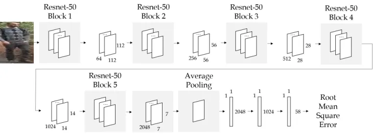
Figure 2: The network architecture for our proposed deep foreground mod-elling method. Images are re-scaled to 224×224 pixels and passed through the convolutional layers of the ResNet-50 network [19]. We take the POOL5 Average Pooling layer as output of the ResNet-50 model, flatten the output, and finally concatenate with two Fully Connected layers. The output layer contains 58 units representing the (x, y) coordinates of skeleton key-points (joints and width markers). We use the RMSProp [20] optimizer and a Mean Squared Error Loss.

Fig 3).

The CNN takes a Re-ID image as input and outputs the key-point

loca-tions as output. To take advantage of transfer learning, we use pre-trained

weights from the ResNet-50 architecture [19] and therefore all input images

are resized to have resolutions 224×224 pixels. The fully connected layers

of this network are modified and we replace them with fully-connected layers

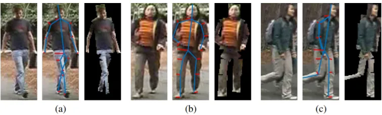
Figure 3: Three examples of a triplet of original images, a skeleton and an image mask that can be produced from the skeleton. Any part of the image within the image mask is considered foreground.

2.2

Foreground feature extraction and feature

weight-ing

Given a predicted skeleton, an image mask/silhouette of a person is generated

by taking rectangular regions for the torso and limb sections (given the joint

key-point locations and the width markers). Examples of skeletons and their

corresponding image masks can be seen in Fig 3. The predicted foreground

area is then used to localise the calculation of two types of image features:

LOMO [17] features and Salient Colour Names [6] features.

2.2.1 LOMO and Weighted LOMO

LOMO [17] features consist of joint HSV histograms and SILTP [18]

a 5 pixel overlap in each dimension. For each row of patches, the maximum

value in each histogram bin is taken as the final descriptor. As in our previous

work [10], we modify LOMO so that features are primarily extracted from

the foreground areas. Each patch is weighted by the percentage of predicted

foreground pixels within the patch:

fw(B) =

|F ∩B|

|B| f(B), (1)

whereB is all pixels within the patch, andF is all pixels labelled foreground.

Therefore, for each row, the maximum value for each histogram bin is more

likely to be taken from the foreground area. We concatenate these features

and the original LOMO features to create Weighted LOMO.

2.2.2 Salient Colour Names

Salient Colour Names [6] features defines sixteen coordinates in the RGB

colour space which each represent a colour, such as fuchsia, blue, aqua and

lime etc. The process is a form of vector quantisation, creating a mapping

from pixel values in the RGB colour space to a colour name distribution

amongst a set of fixed colours. We extract a sixteen-bin Salient Colour

log transform, and normalise it to unit length. We then concatenate these

features to form our final feature descriptor. By localising to limbs, the colour

features are made approximately person-pose invariant: different parts of the

colour feature vector representing a person’s clothing, distinguishing tops

from trousers, shorts and skirts.

2.3

Distance Metric Learning

Distance Metric Learning (DML) is a way to find a subspace mapping of

fea-tures in which distances between matching identities is minimised. KISSME [21]

was the first major DML used for Person Re-Identification, and it calculates

the distance between two feature vectors as:

τ_M2 (fi,fj) = (fi−fj)T(Σ−_I1−Σ−_E1)(fi−fj). (2)

where the intra-personal, ΣI, and extra-personal, ΣE, scatter matrices are

sample estimates from training data. Several methods have since expanded

on KISSME, such as Cross-view Quadratic Discriminant Analysis (XQDA) [17].

Whereas KISSME applies PCA to the input vectors prior in estimating ΣI

dimension-ality reduction stages, XQDA performs DML and dimensiondimension-ality reduction

stages together. IfDis the original dimensionality of the data, andRthe

re-duced dimensionality, XQDA learns a subspace W = (w1,w2, ...,wR)∈RR,

whilst simultaneously learning a distance function:

dw(fi,fj) = (fi−fj)TW(Σ 0₋₁

I −Σ

0₋₁ E )W

T_(f

i−fj) (3)

where Σ0_I = WTΣIW and Σ0_E = WTΣEW. Using the the Generalised

Rayleigh Quotient

J(w) = w

T_Σ Ew

wT_Σ

Iw

(4)

as the objective function, it can be shown that the solution vectors w are

found by a generalised eigenvalue decomposition by maximising:

max

w w

T

ΣEw, s.t.wTΣIw= 1. (5)

Here, for training the XQDA Distance Metric, we use the features extracted

3

Results and Discussion

We investigate the performance of our methods on three of the main Re-ID

data sets:

• VIPeR [1] consists of 632 image pairs, captured using two different

cameras. Images have a resolution of 128×48 pixels, and exhibit large

variation in pose and illumination.

• QMUL GRID [2, 3, 4] consists of 250 image pairs taken using eight

different cameras in an underground rail system. In addition, there are

775 additional images which do not share an identity with an individual

from the 250 image pairs. Images from the QMUL GRID data set have

various different aspect ratio and resolutions, and suffer from large

variation in pose and illumination. Additionally, occlusion and image

capture noise are common in this data set.

• CUHK03 [5] is a larger data set, consisting of 1467 people with up to

ten images per person, taken from a series of camera pairs at various

image resolutions. As the images were taken over a period of several

months, large variation in illumination is seen. This data set also suffers

For all three data sets, we initially train the fully-connected layers of

our ResNet-50 based CNN using pre-trained weights, and follow by training

all layers from ResNet-50’s third stage onwards. We use the RMSProp [20]

optimizer with a learning rate of 0.001.

We split VIPeR in to 316 training/validation identities and 316 testing

identities. We randomly assign 80% of the training/validation identities as

training identities, and the remaining for validation. As deep approaches

require more data than traditional ones, so we expand the size of the training

and validation sets by taking all images from the QMUL GRID data set. For

QMUL GRID, we split the identities into two sets - those which form an image

pair and those which do not form a pair. We then take 80% of each set for

training and 20% for validation. Separating the identities in this way allows

us to have a consistent number of training and validation images between

folds. We train for fifteen epochs with a batch size of 32. After skeleton

prediction, we resize all images to the standard resolution of 128×48 pixels,

rescaling all skeletons to the new size. Examples of the skeleton fitting on

the VIPeR data set can be seen in Fig 4. Following the skeleton fitting and

feature extraction, due to the XQDA distance metric learning stage requiring

Distance Metric. We run our experiments ten times, averaging to produce

the final results.

From Table 1, we can see that our Deep Neural-Network Appearance

Modelling (DNAM) method performs better than other methods at

Rank-10 and Rank-20, but does not perform as well our Partial Least Squares

(PLSAM) method at Rank-1 and Rank-5. When compared to using only

the original LOMO features, we can see an increase of 5.0% in the Rank-1

rate, but a decrease of 1.0% when compared to the PLS skeleton fitting. We

believe that this is because the skeleton fitting between both PLS and Deep

CNN methods are similar, with the Deep Network method having a lower

average Root Mean Squared Error. The CMC curve can be seen in Fig 6.

For QMUL GRID, we split the data set into 125 training/validation

iden-tities and 125 testing ideniden-tities, with all images of ideniden-tities which do not

belong to an image pair being added to the testing gallery set. We

sup-plement the training/validation set with the entirety of the VIPeR data set,

and again assign 80% of the identities from the combined data set as training

identities, with the remaining being validation identities. Also, similar to the

experimentation on the VIPeR data set, we combine the training and

Figure 4: Examples of ground-truth, deep predicted skeletons and PLS pre-dicted skeletons on the VIPeR [1] data set: (a) An example image with a RMSE of 6.5 pixels when using the deep method, and 7.6 pixels when using the PLS method; (b) The image with the minimum RMSE when using the deep method of 1.5 pixels, with the same image having an RMSE of 2.9 pix-els when using the PLS method; (c) The image with the maximum RMSE when using the deep method of 17.9 pixels, with the same image having an RMSE of 12.3 pixels when using the PLS method. The average RMSE when using the deep method was 4.5 pixels, with the average when using the PLS method being 5.2 pixels.

a batch size of 16. After skeleton prediction, we again resize all images to

the standard resolution of 128×48 pixels, rescaling all skeletons accordingly.

Examples of the skeleton fitting on the QMUL GRID data set can be seen

in Fig 5. We again run our experiments ten times, averaging to produce the

final results.

From Table 1, we can see that the best results are obtained from the Deep

CNN based skeleton fitter. When compared to using only the original LOMO

features, we achieve a 11.1% increase in the Rank-1 rate, and an increase of

VIPeR QMUL GRID r=1 r=5 r=10 r=20 r=1 r=5 r=10 r=20 DNAM(v2) 45.3 74.8 86.4 94.2 28.4 49.2 60.0 68.8

DNAM(v1) 42.3 71.4 81.9 91.8 24.3 41.6 52.4 61.8 PLSAM(v2) [10] 46.3 75.0 85.6 93.9 26.7 47.9 59.0 68.2 PLSAM(v1) [10] 42.8 71.9 82.0 91.9 23.9 41.8 51.0 61.4 DeepDiff [22] 43.2 68.0 77.6 86.1 - - - -Null Space [23] 42.3 71.5 82.9 92.1 - - - -MLAPG [24] 40.7 69.9 82.3 92.4 16.6 33.1 41.2 53.0 DeepList [25] 40.5 69.2 81.0 91.2 - - - -LOMO+XQDA [17] 40.3 68.3 80.9 91.1 17.3 36.3 44.8 55.4

SCNCD [6] 37.8 68.5 81.2 90.4 - - - -PKFM [26] 36.8 70.4 83.7 91.7 16.3 35.8 46.0 57.6 CSBT [27] 36.6 66.2 - 88.3 - -

-DCML [28] 33.6 62.9 76.5 87.6 - - -

-Table 1: Results on the VIPeR [1] and QMUL GRID [2, 3, 4] data sets. The best results are shown in bold. (v1) refers to the Weighted LOMO features and XQDA, whereas (v2) refers to the Weighted LOMO features with the Salient Colour Names features and XQDA.

see from Fig 5 that the average Root Mean Squared Error for both the Deep

and PLS methods are similar, with only 0.2 pixels between them. Generally,

the PLS method varies less from the mean skeleton when compared to the

Deep CNN method, which fits limbs in more unusual positions better. The

CMC curve is shown in Fig 6.

For CUHK03, we use the manually cropped version of the images. We

split the data set into 1160 training identities and 100 testing identities, with

CUHK03

r=1 r=5 r=10 r=20 DNAM(v2) 62.2 88.0 94.2 97.5 DNAM(v1) 61.9 88.2 94.2 97.5 PLSAM(v2) [10] 65.2 89.8 95.0 97.9 PLSAM(v1) [10] 64.6 89.2 94.9 98.1

DeepDiff [22] 62.4 87.9 93.6 96.7 Null Space [23] 58.9 85.6 92.5 96.3 MLAPG [24] 58.0 87.1 94.7 98.0 DeepList [25] 55.9 86.3 93.7 98.0 CSBT [27] 55.5 84.3 - 98.0 LOMO+XQDA [17] 54.9 85.3 92.6 97.1 FPNN [5] 20.7 50.9 67.0 83.0

Table 2: Results on the CUHK03 [5] data set. The best results are shown in bold. (v1) refers to the Weighted LOMO features and XQDA, whereas (v2) refers to the Weighted LOMO features with the Salient Colour Names features and XQDA.

As we do not have any ground-truth, hand-labelled skeleton data for the

CUHK03 data set, we instead train the Deep CNN based skeleton fitter on

the VIPeR and QMUL GRID data sets. We divide the entire VIPeR and

QMUL GRID data sets into training/validation/testing sets as described for

the previous two data sets. We train for fifteen epochs with a batch size of

32. However, as the source images for CUHK03 are a higher resolution as

compared to VIPeR and QMUL GRID, we instead scale to 160×60 pixels

for feature extraction. We run our experiments twenty times, averaging to

Figure 5: Examples of ground-truth, deep predicted skeletons and PLS pre-dicted skeletons on the QMUL GRID [2, 3, 4] data set: (a) An example image with a RMSE of 4.3 pixels when using the deep method, and 4.5 pixels when using the PLS method; (b) The image with the minimum RMSE when using the deep method of 2.2 pixels, with the same image having an RMSE of 3.9 pixels when using the PLS method; (c) The image with the maximum RMSE when using the deep method of 18.3 pixels, with the same image having an RMSE of 17.6 pixels when using the PLS method. The average RMSE when using the deep method was 5.5 pixels, with the average when using the PLS method being 5.3 pixels.

the deep method. We believe this is due to it generalising better when an

unseen image from an unseen data set is passed to the model. In addition,

whilst the VIPeR and QMUL GRID data sets are mainly person images of

the front or back of a person, CUHK03 is roughly half frontal or back-facing

and half side-facing. The use of a single model for the Deep CNN method

versus the two used in the PLS method lead to it fitting a frontal skeleton

4

Conclusions

In this paper, we propose a deep CNN based method to fit skeletons to Re-ID

images and estimate foreground regions, including head, torso and limbs. We

compare the results with a linear appearance based skeleton fitting which

uses Partial Least Squares and evaluate the results of both methods in a

Re-ID matching framework. For both methods, training images and

cor-responding ground-truth, hand-labeled skeleton information can be used to

build a model to predict the skeleton of a person. From this we have shown

that more accurate skeletons can be predicted by using the Deep CNN based

model, particularly on unusual person body poses. For the matching, LOMO

and Salient Colour Names features are extracted and weighted according to

their spatial position in the person image, i.e. ordered by pose information

from the foreground estimation. Once extracted, these features are further

weighted by XQDA Distance Metric Learning technique for matching. We

have demonstrated that by using foreground modelling and weighting the

features, we can achieve superior matching performance. Experiments on

the VIPeR, QMUL GRID and CUHK03 data sets, and at best our proposed

methods achieve 6%, 11.1% and 10.3% improvement respectively when

We have also demonstrated that both of our proposed methods generalise

well between data sets. Specifically, in the case of CUHK03, we are able to

achieve good skeleton fitting results even though the models were trained

only on VIPeR and QMUL GRID. This generalisability is important since

CNN approaches require large amounts of training data to be accurate.

Fur-thermore, while the PLS method required separate models for frontal and

sideways views, the Deep CNN method because of its non-linearities, is able

to learn a single model for this task. However, the majority of images used

for training the skeleton prediction model were of people facing directly

to-wards or away from the camera, with the occasional sideways-facing image.

Future work will investigate how to re-train the model using a more balanced

variety of camera directions and skeleton poses, and whether some form of

body pose augmentation can be incorporated into the training regime.

An obvious and necessary extension of this work is to combine the deep

CNN skeleton prediction into a Deep CNN matching framework, thus

pre-cluding the need for feature extraction and distance metric learning. One

approach which seems viable is to use the limb localisations to partition the

image input into regions of interest boxes extracted and arranged in a grid,

usefully leveraged for deep feature learning.

5

Acknowledgements

The authors gratefully acknowledge funding by the UK Engineering and

Physical Sciences Research Council (grant no. EP/L016400/1), the EPSRC

Centre for Doctoral Training in Urban Science.

References

[1] D. Gray, S. Brennan, and H. Tao, “Evaluating appearance models for

recognition, reacquisition, and tracking,” in Proc. IEEE International

Workshop on Performance Evaluation for Tracking and Surveillance

(PETS), 3(5), 1–7, Citeseer (2007).

[2] C. Liu, S. Gong, C. C. Loy, et al., “Person re-identification: What

features are important?,” in European Conference on Computer Vision,

391–401, Springer (2012).

[3] C. C. Loy, T. Xiang, and S. Gong, “Multi-camera activity correlation

2009. IEEE Conference on, 1988–1995, IEEE (2009).

[4] C. C. Loy, T. Xiang, and S. Gong, “Time-delayed correlation

analy-sis for multi-camera activity understanding,” International Journal of

Computer Vision 90(1), 106–129 (2010).

[5] W. Li, R. Zhao, T. Xiao, et al., “Deepreid: Deep filter pairing neural

network for person re-identification,” in Proceedings of the IEEE

Con-ference on Computer Vision and Pattern Recognition, 152–159 (2014).

[6] Y. Yang, J. Yang, J. Yan, et al., “Salient color names for person

re-identification,” in European conference on computer vision, 536–551,

Springer (2014).

[7] C. Liu, S. Gong, and C. C. Loy, “On-the-fly feature importance

min-ing for person re-identification,” Pattern Recognition 47(4), 1602–1615

(2014).

[8] M. Farenzena, L. Bazzani, A. Perina, et al., “Person re-identification

by symmetry-driven accumulation of local features,” in Computer

Vi-sion and Pattern Recognition (CVPR), 2010 IEEE Conference on, 2360–

[9] N. Jojic, A. Perina, M. Cristani,et al., “Stel component analysis:

Mod-eling spatial correlations in image class structure,” in Computer Vision

and Pattern Recognition, 2009. CVPR 2009. IEEE Conference on, 2044–

2051, IEEE (2009).

[10] G. Watson and A. Bhalerao, “Person re-identification using partial least

squares appearance modelling,” in International Conference on Image

Analysis and Processing, 25–36, Springer (2017).

[11] D. Cheng, Y. Gong, S. Zhou, et al., “Person re-identification by

multi-channel parts-based cnn with improved triplet loss function,” in

Proceed-ings of the IEEE Conference on Computer Vision and Pattern

Recogni-tion, 1335–1344 (2016).

[12] H. Zhao, M. Tian, S. Sun, et al., “Spindle net: Person re-identification

with human body region guided feature decomposition and fusion,” in

Proceedings of the IEEE Conference on Computer Vision and Pattern

Recognition, 1077–1085 (2017).

[13] L. Wei, S. Zhang, H. Yao, et al., “Glad: Global-local-alignment

[14] E. Insafutdinov, L. Pishchulin, B. Andres, et al., “Deepercut: A deeper,

stronger, and faster multi-person pose estimation model,” in European

Conference on Computer Vision, 34–50, Springer (2016).

[15] X. Liu, P. Lyu, X. Bai, et al., “Fusing image and segmentation cues

for skeleton extraction in the wild,” in Proceedings, ICCV Workshop on

Detecting Symmetry in the Wild, Venice, 6, 8 (2017).

[16] L.-C. Chen, G. Papandreou, I. Kokkinos, et al., “Deeplab: Semantic

image segmentation with deep convolutional nets, atrous convolution,

and fully connected crfs,” arXiv preprint arXiv:1606.00915(2016).

[17] S. Liao, Y. Hu, X. Zhu,et al., “Person re-identification by local maximal

occurrence representation and metric learning,” in Proceedings of the

IEEE Conference on Computer Vision and Pattern Recognition, 2197–

2206 (2015).

[18] S. Liao, G. Zhao, V. Kellokumpu, et al., “Modeling pixel process with

scale invariant local patterns for background subtraction in complex

scenes,” in Computer Vision and Pattern Recognition (CVPR), 2010

[19] K. He, X. Zhang, S. Ren,et al., “Deep residual learning for image

recog-nition,” in Proceedings of the IEEE conference on computer vision and

pattern recognition, 770–778 (2016).

[20] T. Tieleman and G. Hinton, “Lecture 6.5-rmsprop: Divide the gradient

by a running average of its recent magnitude,” COURSERA: Neural

networks for machine learning 4(2), 26–31 (2012).

[21] M. Koestinger, M. Hirzer, P. Wohlhart, et al., “Large scale metric

learning from equivalence constraints,” in Computer Vision and

Pat-tern Recognition (CVPR), 2012 IEEE Conference on, 2288–2295, IEEE

(2012).

[22] Y. Huang, H. Sheng, Y. Zheng, et al., “Deepdiff: Learning deep

differ-ence features on human body parts for person re-identification,”

Neuro-computing 241, 191–203 (2017).

[23] L. Zhang, T. Xiang, and S. Gong, “Learning a discriminative null space

for person re-identification,” in Proceedings of the IEEE Conference on

[24] S. Liao and S. Z. Li, “Efficient psd constrained asymmetric metric

learn-ing for person re-identification,” in Proceedings of the IEEE

Interna-tional Conference on Computer Vision, 3685–3693 (2015).

[25] J. Wang, Z. Wang, C. Gao,et al., “Deeplist: Learning deep features with

adaptive listwise constraint for person reidentification,” IEEE

Trans-actions on Circuits and Systems for Video Technology 27(3), 513–524

(2017).

[26] D. Chen, Z. Yuan, G. Hua, et al., “Similarity learning on an explicit

polynomial kernel feature map for person re-identification,” in

Proceed-ings of the IEEE Conference on Computer Vision and Pattern

Recogni-tion, 1565–1573 (2015).

[27] J. Chen, Y. Wang, J. Qin,et al., “Fast person re-identification via

cross-camera semantic binary transformation,” in IEEE Conference on

Com-puter Vision and Pattern Recognition, (2017).

[28] N. McLaughlin, J. M. del Rincon, and P. C. Miller, “Person

reidentifica-tion using deep convnets with multitask learning,” IEEE Transactions

[29] R. Zhao, W. Ouyang, and X. Wang, “Learning mid-level filters for

per-son re-identification,” in Proceedings of the IEEE Conference on

Com-puter Vision and Pattern Recognition, 144–151 (2014).

Gregory Watson is a PhD candidate at the Department of Computer

Sci-ence at the University of Warwick, and a member of the Centre for Doctoral

Training in Urban Science & Progress. He received his MEng in Computer

Science from the University of Warwick in 2015. His current research

in-clude using deep learning and foreground modelling to improve person

re-identification.

Abhir Bhalerao, PhD, is an Associate Professor in Computer Science at

the University of Warwick, UK. He has been an active researcher in medical

image analysis and computer vision for over 25 years. He has published

around 80 refereed articles in image analysis, medical imaging, graphics and

computer vision. His current research interests are in modelling knee and

spinal disorders from MRI, biometrics and person re-identification, and vision