Scheduling of multi-class multi-server queueing systems
with abandonments
∗U. Ayestab,c,e,f, P. Jackod, V. Novaka
aCERGE-EI, a joint workplace of Charles University in Prague and the Economics Institute of the Czech Academy of Sciences,
Politickych veznu 7, Prague 1, 111 21, Czech Republic bCNRS, LAAS, 7 avenue du colonel Roche, 31400 Toulouse, France cIKERBASQUE, Basque Foundation for Science, 48011 Bilbao, Spain
dLancaster University, Department of Management Science, Lancaster, LA1 4YX, UK eUPV/EHU, Univ. of the Basque Country, 20018 Donostia, Spain
fUniv. de Toulouse, INP, INSA, LAAS, 31400 Toulouse, France
This is the author final version of the article published in Journal of Scheduling, online on 11 November 2015, DOI 10.1007/s10951-015-0456-7.
Abstract
Many real-world situations involve queueing systems in which customers may abandon if service does not start sufficiently quickly. We study a comprehensive model of multi-class queue scheduling accounting for customer abandonment, with the objective of minimizing the total discounted or time-average sum of linear waiting costs, completion rewards and aban-donment penalties of customers in the system. We assume the service times and abandoning times are exponentially distributed. We solve analytically the case in which there is one server and there are one or two customers in the system and obtain an optimal policy. For the gen-eral case, we use the framework of restless bandits to analytically design a novel simple index rule with a natural interpretation. We show that the proposed rule achieves near-optimal or asymptotically-optimal performance both in single- and multi-server cases, both in overload and underload regimes, and both in idling and non-idling systems.
1
Introduction
Abandonment (aka reneging) is a ubiquitous phenomenon in a multitude of systems. It may happen due to customers’ impatience, mobility, perishability, obsolescence, or other reasons. For instance, customers can abandon after waiting for too long in a queue, Internet users may give up a transfer if the connection is slow, or external factors may cause customers not to be amenable to service anymore. Abandonment is especially important in call centers (Gans et al. 2003,Aksin et al. 2007) and health care (Argon et al. 2010). Other application areas in which abandonment may have a significant impact are real-time systems where data received after certain hard dead-line is useless (Buttazzo 2011), or inventory systems with perishable goods (Graves 1984).
∗
Customer abandonment has a very negative impact on performance both from the cus-tomer’s and the system’s perspective. A customer who decides to abandon perceives that the system is poorly managed or not well dimensioned, which may lead to switching to a competi-tor. In health care, abandonment may be used to model irreversible deterioration of patients’ health. From the system’s point of view the abandonment might imply that resources have been wasted by allocating them to a customer that decided to abandon anyway. For this reason it is important to design efficient scheduling policies in the presence of abandonment.
Mathematically, abandonment can be studied by queueing models, but as a consequence of the complexity, the problem of how to schedule impatient customers is not completely under-stood. For instance, very little is known about how to schedule customers in order to optimize a performance criteria that may depend on the number of customers waiting and on the number of customers that abandon the queue. This is an important question, for which no general so-lution is known, and it is likely to be computationally infeasible. The main focus of the present paper is to design a simple implementable scheduling rule for multi-class systems that shows a nearly-optimal performance.
The literature on models that incorporate customer abandonment is rich, and there has been a surge in recent years motivated by their application in health-care, call-centers and the Internet. As an illustration of the latter we can mention the recent Special Issue in Queueing Systems de-voted to queueing systems with abandonmentsHasenbein and Perry(Eds). An important stream of works investigate the performance of single-server systems in the presence of abandonment (see for example Iravani and Balcio ˘glu 2008, Baccelli et al. 1984, Brandt and Brandt 2004, Brill and Posner 1977,Ata and Tongarlak 2013), and there is also a significant body of literature deal-ing with the multi-server case (see for example Boxma and de Waal 1994,Boots and Tijms 1999,
Whitt 2004). We also refer toDai and He(2012) for a recent survey on multi-server systems with abandoning customers. Abandonment systems have also been looked at from a game-theoretic perspective (seeHassin and Haviv 2003, Chapter 5, and references therein). More relevant to our work are the papers that deal with the control of systems in the presence of abandonment (see, for example,Harrison and Zeevi 2004,Glazebrook et al. 2004,Argon et al. 2010,Down et al. 2011,
Jouini et al. 2010,Atar et al. 2010). The most common objectives are either service completion reward maximization or waiting cost and abandonment penalty minimization. In Glazebrook et al.(2004) the authors consider three different models for service completion reward maximiza-tion, and derive heuristic rules using a variety of techniques. Argon et al. (2010) study how to schedule optimally in a patient triage problem. Down et al.(2011) deals with a two-class system and derives sufficient conditions for a classic priority rule to be optimal. InJouini et al.(2010) the authors derive scheduling policies for call centers with two classes of customers.
1.1 Problem Description
In this paper we aim at solving the problem of multi-class multi-server customer scheduling for a system in which we allow for abandonment. The objective is to maximize the total discounted or time-average revenue from customers in the system, where the revenue is defined as the sum of service completion rewards minus waiting costs and abandonment penalties. In contrast toAtar et al. (2010) and most of the previous literature,the customers in service are also charged a waiting cost, which as we will see, will have significant consequences.
Service completion times and abandonment times are exponentially distributed. Thus, the
class-k customer’s behavior is completely characterized by the mean service time1/µk (with service
rateµk >0while served), the mean abandonment time1/θk(with abandonment rateθk >0while
not served), the waiting cost rate ck (possibly negative), the abandonment penaltydk (possibly
negative), and the service completion reward rk(possibly negative). Future costs, penalties and
rewards are discounted with exponential discount rateα≥0.
We emphasize that we assume that the customers in service cannot abandon, though our approach could easily be adapted to the other possibility. We also assume that a customer can only receive service from one server at a time. Customers are assumed independent of each other, i.e., we assume that at any moment and independently of everything else, every customer (except for those in service, if any) may abandon the system, while a customer in service leaves the system if her service is completed.
It is further permitted to allocate each server to analternative task (such as idling, battery recharging or service maintenance), for which we obtain an alternative-task reward rateκ. Thus we assume there are M alternative tasks — one for each server. For instance, the role of this alternative task with a positiveκcould be to allocate a server to it when all the customers in the system have a relatively low profitability (e.g., low service completion reward, low waiting cost, and low abandonment penalty). On the other hand, by setting this parameter to a large negative value we may force a server to be non-idling (whenever there are waiting customers). Ifκ=−∞, then the alternative task will never be engaged, and we call this thenon-idling variant. Finally, if
κ = 0, then the alternative task represents the classic possibility of server idling and we call this theidling variant.
The joint goal is to maximize the expected aggregate rate of service completion rewards and alternative-task rewards minus the waiting costs and abandonment penalties, over an infinite horizon. The server is assumed to bepreemptive(i.e., the service of a customer or of the alternative task can be interrupted at any moment). Thus, the servers continuously decide which customer (if any) to serve.
The most relevant paper for our work is Atar et al. (2010), where the authors investigate this model under the time-average criterion and introduce the cµ/θ-rule for the in-queue cost minimization problem (i.e., the customers in service do not incur the waiting cost):
Rule 1 (cµ/θ-rule) Assign to each customer of classkin the system the following index rate: (ck+dkθk)µk
θk
and allocate the servers to theM customers with the highest rates.
It is shown inAtar et al.(2010) (and extended inAtar et al.(2011) to a general service dis-tribution for a non-preemptive server) that thecµ/θ-rule minimizes asymptotically (in the multi-server fluid limit sense) the time-averagein-queuewaiting cost in the overload case (i.e., when the system would be unstable if no abandonment were possible) under Poisson arrivals.
If there is no abandonment (i.e., θk = 0for all classes k), then this problem recovers the
classic job scheduling problem considered in Cox and Smith (1961),Smith (1956), Fife (1965),
Buyukkoc et al.(1985), for which the following rule is optimal in a single-server setting (M = 1) under Poisson arrivals, for both the discounted and time-average criterion:
Rule 2 (cµ-rule) Assign to each customer of class k in the system the following index rate: ckµk and
allocate the servers to theM customers with the highest rates.
For a given class k, ckµk measures the expected savings in waiting costs if a customer of
1.2 Main Contributions
The most important contributions of the paper are as follows:
• We develop a newversatile modeling framework to optimize the performance of non-work-conserving queueing systems, by formulating the system with abandonments as a multi-armed restless bandit problem, which is relatively easily generalizable to include more complex system features;
• Using this stochastic optimization framework, we derive anovel, robust, and simple scheduling rule, and provide its intuitive interpretation;
• We show that the proposed rule achievesnear-optimal and asymptotically-optimal performance both in single- and multi-server cases, both in overload and underload regimes, and both in idling and non-idling systems, which apart from its own sake validates the framework.
The most interesting case for practical implementation is the time-average criterion on which we focus next. Let us denote byCk:=rk+dk−ck(1/µk−1/θk)theexpected total profit, since
it is the difference between the expected total revenue if serving the customer always (rk−ck/µk)
and the expected total revenue if not serving her at all (−dk−ck/θk). Our stochastic optimization
approach yields the following Whittle Index rule (WI rule) that we propose to be implemented in practice:
Rule 3 (WI rule) Assign to each customer of class k in the system the following index rate: Ckµk, if
Ck ≥ 0andCkθk, otherwise, and to each alternative task kthe following index rate: κ, and allocate the
servers to theM options with the highest rates.
There is a simple interpretation of the WI index rate, as measuring theexpected profit rate, since the expected total profitCkis divided by the expected time the customer stays in the system,
which is1/µkif it is preferable to serve and1/θkif it is preferable not to serve.
We also emphasize the fundamental differences between our approach and results and those of the existing literature on control of systems with abandonments, to the best of our knowl-edge:
• this is thefirst paper that tries to solve the original stochastic problem. Previous literature focused on solving simpler limiting regimes such as deterministic fluid limits, equilibria in overload, or diffusions;
• this is thefirst paper that considers the discounted criterion, and we derive our rule under both the discounted and the time-average criterion. Moreover, our rule is optimal if θk → 0(it
reduces to thecµrule) and gives a simple priority index in general;
1.3 Paper Structure
The problem as described above is hard to solve for optimality, and therefore we approach it by solving it approximately by using several levels of problem relaxation. Section 2 contains the formulation of the problem without arrivals as a Markov Decision Process after its uniformiza-tion and discretizauniformiza-tion. This formulauniformiza-tion can be seen as a generalizauniformiza-tion of the job sequencing problem with geometrically distributed service times formulated in Cox and Smith(1961), who showed that the index rule based on thecµindex is optimal. The modeling framework is known as the multi-armed restless bandit problem, an extremely difficult optimization problem that has been proven PSPACE-hard (Papadimitriou and Tsitsiklis 1999), that is, its complexity grows ex-ponentially in time and in memory requirements. The term restless refers to the fact that, as a consequence of abandonment, the state of all customers in the system varies in time regardless of whether they are served or not. Restless problems can be solved analytically only in a few cases (typically with largely restricted dynamics), and this explains to some extent why optimality re-sults on scheduling in systems with abandonment are so scarce in queueing theory.
In Section 3we solve analytically the case in which there are one or two customers in the system. The case with one customers gives a fundamental insight into the problem and provides an interpretation of Ck. For the case with two customers we characterize in closed form the
optimal switching curve which gives rise to a simple rule. This rule is not an index rule because it is not separable - the decision to serve one customer cannot be made by just comparing indices for each customer where the index for one customer depends only on that customer’s parameters and not those of the other one.
To approach the intractable case with more than two customers, we follow the approach of Whittle(1988) which allows us to derive a scheduling rule for any number of customers and servers by calculating the Whittle indices as described in Ni ˜no-Mora (2007). In Section 4 we introduce the relaxed formulation of the original problem. The main idea is to relax the sample path constraint (that imposes that exactly M options be served at a time) by letting the time-average/discounted number of options served in a period be M. This relaxation significantly simplifies the problem. The optimal policy of the relaxed formulation becomes now separable across options, that is, we can calculate for each customer the Whittle index value (that depends only on the customer’s parameters and on whether she is still waiting or not), and the optimal scheduler serves in every period the customers with actual Whittle index value higher than a threshold (the value of the threshold ensures that the time-average number of customers served is preciselyM).
Section 5 contains the main contribution of this paper, that is, the analysis of the relaxed problem and the heuristic rule for the original stochastic optimization formulation. The optimal policy for the relaxed problem need not be feasible for the original problem, yet it allows us . We calculate the Whittle index values, which can be interpreted as dynamic shadow prices, in closed form, and derive their equivalents for the continuous-time problem in order to construct a heuristic Whittle index rule for the original problem with arrivals. The Whittle index rule is feasible (at mostMcustomers are served at a time) and is typically reported to have an extremely good performance (Ni ˜no-Mora 2007). In addition, it was shown inWeber and Weiss(1990) that such a heuristic approaches optimality in the limit as the number of customers and the number of servers grows (under certain additional assumptions).
broad range of parameters and scenarios. From this section we can conclude that: (i) the WI rule outperforms or is equivalent to thecµ/θ-rule, (ii) when there is a class of customers withθlarger thanµ, or whenc’s differ across classes, then the WI rule can significantly outperformcµ/θ, (iii) in cases in which the optimal scheduling policy chooses to idle instead of serving, the WI rule is much better thancµ/θorcµ, (iv) in many scenarios the WI rule is equal to the optimal policy for a broad setting of the parameter values.
Proofs are deferred to the appendix to streamline the paper.
2
MDP Formulation
Since thecµ-rule is optimal both under Poisson arrivals and under no arrivals, we set out to an-alyze the continuous-time model without arrivals. Our aim is to obtain a rule accounting for abandonment whose performance in the continuous-time model with arrivals we later evaluate by means of numerical experiments. We set the model in the framework of the dynamic and sto-chastic resource allocation problem, closely followingJacko(2009). We assume there are initially
K customers, i.e. one of each class.
We will uniformize and discretize the problem described in the previous section. Let us consider any sufficiently large uniformization rate (per second) γ, which can be interpreted as the number of periods per second. In other words,1/γis the expected duration in seconds until the next event happens, which will be taken in the discretization as the duration of a discrete-time period. The uniformization and discretization is described in Table 1. In the following we suppose that the parameters are uniformized and discretized.
Remark 1 In our model without arrivals we require γ ≥ Mmaxk∈Kµk +Kmaxk∈Kθk for both the
discounted and time-average problem. One might consider including the rateα in the uniformization in order to use a commonγ for both cases and then to setγ = 1without loss of generality, so that the same parameters can be interpreted as probabilities in the discrete-time, uniformized version. This would be perfectly valid in the undiscounted case. However, we were unable to use similar tricks that would work for the discounted case (which is central to our analysis). For instance, defining γ ≥ Mmaxk∈Kµk+
Kmaxk∈Kθk+α and settingγ = 1prohibits consideration of the myopic case (in which α → +∞).
Even when we ignored the myopic case and tried to redo the whole analysis, we did not obtain the same index. One of the important issues is that the index in the discretized case is a value “per period”, while in the continuous case it is rate “per second”. We make this distinction insubsection 5.4and relate it to the Lagrangian parameterν, which is the discretized work charge, andξ, the corresponding rate.
After the problem has been uniformized, we formulate the problem as a discrete time Markov Decision Process (MDP). Consider the time slotted into epochs t ∈ T := {0,1,2, . . .}
at which decisions can be made. The time epochtcorresponds to the beginning of the time pe-riod t. Att = 0there areK customers (labeled byk ∈ K) and M alternative tasks (labeled by
k ∈ M := {K + 1, . . . , K +M}) awaiting service. Thus, there areK +M competing options, labeled byk ∈ K+ := K ∪ M. At each time epocht, the decision-maker allocates each server to
exactly one (distinct) option.
2.1 Customers
Parameter per second Parameter per period
arrival rateλk arrival probabilityλ0k:=λk/γ
service completion rateµk service completion probabilityµ0k:=µk/γ
abandonment rateθk abandonment probabilityθk0 :=θk/γ
exponential discount rateα geometric discount factorβ :=γ/(α+γ)
alternative task reward rateκ alternative task rewardκ0:=κ/(α+γ)
waiting cost rateck waiting costc0k:=ck/(α+γ)
work charge rateξ work chargeν :=ξ/(α+γ)
abandonment penaltydk abandonment penaltydk
[image:7.612.135.482.55.183.2]service completion rewardrk service completion rewardrk
Table 1: Uniformization and discretization of continuous-time parameters for the discrete-time model with uniformization factorγ.
zero servers (i.e., “not serving”), and action1means allocating one server (i.e., “serving”). This action space is the same for every customerk.
Each customerkis defined independently of other customers as the tuple
Nk,(Wak)a∈A,(Rak)a∈A,(Pak)a∈A
,
where
• Nk:={0,1}is thestate space, where state0represents a service already completed or aban-doned, and state1means that the service is uncompleted and not abandoned;
• Wak :=
Wk,na
n∈Nk
, where Wk,na is the (expected) one-period capacity consumption, or workrequired by customerkat statenif actionais decided at the beginning of a period; in particular, for anyn∈ Nk,
Wk,n1 := 1, Wk,n0 := 0;
• Rak :=Rak,n
n∈Nk
, whereRak,nis the expected one-periodrevenueearned by customerkat statenif actionais decided at the beginning of a period; in particular,
R1k,0 := 0, Rk,11 :=−c0k,
R0k,0 := 0, Rk,01 :=−c0k−βdkθ0k;
• Pak:=
pak,n,m
n,m∈Nk
is the customer-kstationary one-periodstate-transition probability
ma-trixif actionais decided at the beginning of a period, i.e.,pak,n,mis the probability of moving to statemfrom statenunder actiona; in particular, we have
P1k:=
0 1 0 1 0 1 µ0k 1−µ0k
!
, P0k:=
0 1 0 1 0 1 θ0k 1−θ0k
!
The dynamics of customerkis thus captured by thestate processXk(·)and theaction process
ak(·), which correspond to state Xk(t) ∈ Nk and action ak(t) ∈ A at all time epochs t ∈ T.
As a result of deciding actionak(t)in stateXk(t)at time epoch t, the customerkconsumes the allocated capacity, earns the revenue, and evolves its state for the time epocht+ 1.
Remark 2 The attentive reader might wonder why to allow serving in state0. This is assumed for com-patibility with the methodology derived in the previous literature. It turns out that the index value of state
1 we obtain below would be the same even if serving in state 0was not allowed because the one-period revenue is zero in this absorbing state under both actions. Moreover, the heuristic we propose below only relies on the index value of state1.
Note that we have defined the customer with a zero completion reward. This is without loss of generality, because the customers with a non-zero completion reward can be normalized to a cost-only customer as follows. The following proposition follows trivially from the model description.
Proposition 1 The expected one-period revenue for a customer with service rate µek, abandonment rate
e
θk, service completion rewardrek, waiting costeckand abandonment penaltydek is equal to the one-period
revenue for a customer with service rateµk = µek, abandonment rateθk = θek, revenuerk = 0, waiting
costck =eck−βerkµk, and abandonment penaltydk =dek+erk
µk
θk.
2.2 Alternative Tasks
We model each alternative task as a staticκ-customerwith a single state0 and with rewardκ0 if served, i.e., such a taskk ∈ Mis defined byNk := {0}, Wk,a0 := a, Rak,0 := κ0a, pak,0,0 := 1for all
a∈ A.
2.3 Unified Optimization Criterion
Before describing the problem we first define an averaging operator that will allow us to discuss the infinite-horizon problem under the traditional β-discounted criterion and the time-average criterion in parallel. LetΠX,a be the set of all the policies that for each time epochtdecide (pos-siblyrandomized) actiona(t)based only on the state-process historyX(0), X(1), . . . , X(t)and on the action-process historya(0), a(1), . . . , a(t−1)(i.e.,non-anticipative). LetEπτ denote the
expecta-tion over the state processX(·)and over the action processa(·), conditioned on the state-process historyX(0), X(1), . . . , X(τ)and on policyπ.
Consider any expected one-period quantityQaX(t()t)that depends on stateX(t)and on action
a(t)at any time epocht. For any policyπ ∈ΠX,a, any initial time epochτ ∈ T, and anydiscount
factor0≤β ≤1we define the infinite-horizonβ-average quantityas1
Bπτ
h
QaX(·)(·), β,∞i:= lim T→∞
T−1 X
t=τ
βt−τEπτ
h
QaX((t)t)
i
T−1 X
t=τ
βt−τ
. (1)
The β-average quantity recovers the traditionally considered quantities in the following three cases:
1For definiteness, we considerβ0
• expected time-average quantitywhenβ = 1.
• expected totalβ-discounted quantity, scaled by constant1−β, when0< β <1;
• myopic quantitywhenβ = 0.
Thus, whenβ = 1, the problem is formulated under thetime-average criterion, whereas when
0 < β < 1the problem is considered under theβ-discounted criterion. The remaining case when
β = 0reduces to a static problem and hence is considered in order to define amyopic policy. In the following we consider the discount factor β to be fixed and the horizon to be infinite, therefore we omit them in the notation and write brieflyBπτ
h
QaX(·)(·)i.
2.4 Optimization Problem
We now describe in more detail the problem we consider. Let ΠX,a be the space of
random-ized and non-anticipative policies depending on the joint state-processX(·) := (Xk(·))k∈K+ and
deciding the joint action-processa(·) := (ak(·))k∈K+, i.e.,ΠX,ais thejoint policy space.
For any discount factorβ, the problem is to find a joint policyπmaximizing thevalue func-tiongiven by theβ-average aggregate revenue starting from the initial time epoch0subject to the family ofsample pathallocation constraints, i.e.,
V(X(0)) := max
π∈ΠX,a Bπ0
X
k∈K+ Rak(·)
k,Xk(·)
(P)
subject to Eπt
X
k∈K+ ak(t)
=M, for allt∈ T
Note that the constraint could equivalently be expressed in words as that for all t ∈ T:
P
k∈K+ak(t) =Munder policyπand for any possible joint state-process historyX(0),X(1), . . . ,X(t).
We say that a policy is Markovian deterministic if it chooses the vector a(t) according to a fixed rule based solely on the current system state X(t). LetΠMD denote the set of Marko-vian deterministic policies. From standard results in Markov decision processes (Puterman 2005, Chapter 6) it follows that there is no loss of generality in restricting our attention to the policies inΠMD.
The solution to problem (P) can be found by determining the unique solutionV(·)to Bell-man’s equation, which forβ <1is
V(x) = max
as.t.P
k∈K+ak=M
X
k∈K+ Rak
k,xk+β
X
y
qxa,yV(y)
(2)
3
Optimal Solution for Special Cases
Problem (P) is hard to solve in its whole generality, but we have identified special cases that admit an analytical solution of the Bellman equation, summarized in this section. To the best of our knowledge these particular have not been considered previously in the literature.
Let us first denote by
Ck: =β
c0k(µ0k−θk0) +dkθk0(1−β+βµ
0
k) (1−β+βθk0)(1−β+βµ0k)
= ck(µk−θk) +dkθk(α+µk) (α+θk)(α+µk)
.
(3)
Proposition 2 Ckis the difference between the expected total revenue if serving the customer always and
the expected total revenue if not serving her at all.
We remark that in the undiscounted caseCksimplifies as follows:
Ck=dk−c0k
1
µ0k −
1
θ0k
=dk−ck
1
µk − 1
θk
. (4)
3.1 Single Customer at a Single Server
In the single server case with a single customer competing with a single alternative task, we introduce the following index value (1U):
νk1U:=Ck. (5)
This index value thus inherits the interpretation from Ck, so it is positive if and only if serving
the customer always is more profitable than not serving her at all.
Proposition 3 LetK = 1,M = 1and the alternative task rewardκ0 = 0. The solution to Problem(P)is: (i) Ifν11U≥0, then it is optimal to serve customer1;
(ii) Ifν11U≤0, then it is optimal to allocate the server to the alternative task (k= 2).
It is important to note that the above result means that idling may be optimal for a very impatient customer.
3.2 Two Customers at a Single Server
In the case of two customers competing among themselves (2U) for a single server, due to the technical complexity of the problem we focus on the undiscounted case (α = 0, i.e.,β = 1). We introduce the followingnon-separable index value for customerk = 1,2with respect to the other customer (3−k):
νk2U:= Ckθ
0
k
θ0k+µ03−k. (6)
We note that this expression is not separable since it depends on the other customer’s parameters, though only through the service rate µ03−k, so does not lead to an index rule in the traditional sense.
Proposition 4 Suppose that K = 2andCk ≥ 0for k ∈ K. The following holds for problem(P) with
M = 1,α= 0, and the alternative task rewardκ0 =−∞:
(i) Ifν12U≥ν22U, then it is optimal to serve customer1;
(ii) Ifν12U≤ν22U, then it is optimal to serve customer2.
4
Relaxations and Decomposition
For larger values ofK andM, the problem is analytically intractable, and therefore we approach it in a different way. The main idea is to solve a relaxed version of the problem (P). It turns out that the relaxation will in fact allows decomposition of the problem, and the optimal solution to the relaxed problem can be obtained by solving parametric single-option subproblems. In
Section 5we will then show how the solution of the relaxed problem can be used to construct a nearly-optimal heuristic for the original problem (P).
4.1 Relaxations
We can use the fact thatWak(t)
k,Xk(t) =ak(t)(cf. definitions inSection 2) and instead of the constraints
in (P), for notational reasons, we consider the sample pathconsumptionconstraintsEπt
h P
k∈K+W
ak(t)
k,Xk(t)
i
=
M, for allt∈ T. These constraints imply theepoch-texpectedconsumption constraints,
Eπ0
X
k∈K+ Wak(t)
k,Xk(t)
=M, for allt∈ T (7)
requiring that the capacity be fully allocated at every time epoch if conditioned on X(0)only. Finally, we may require this constraint to hold only onβ-average, as theβ-average capacity con-sumption constraint
Bπ0
X
k∈K+ Wak(·)
k,Xk(·)
=Bπ0 [M]. (8)
UsingBπ0 [M] =M, we obtain the followingrelaxationof problem (P),
max
π∈ΠX,a Bπ0
X
k∈K+ Rak(·)
k,Xk(·)
(PW)
subject to Bπ0
X
k∈K+ Wak(·)
k,Xk(·)
=M.
This relaxation was introduced inWhittle(1988), and it gives us the following result.
The Whittle relaxation (PW) can be approached by traditional Lagrangian methods, intro-ducing a Lagrangian parameter, say ν, interpreted as thework charge, to dualize the constraint, obtaining the following Lagrangian relaxation,
max
π∈ΠX,a Bπ0
X
k∈K+ Rak(·)
k,Xk(·)−ν
X
k∈K+ Wak(·)
k,Xk(·)
+νM. (PLν)
The classic Lagrangian result is the following:
Proposition 6 For anyν, problem(PLν)is a relaxation of problem(PW), and further a relaxation of problem (P). Moreover, (PLν)for every ν provides an upper bound for the optimal value of both problem(PW)and problem(P).
4.2 Decomposition into Single-Option Subproblems
We now set out to decompose the optimization problem (PL
ν) as is standard for Lagrangian re-laxations, considering ν as a parameter. Notice that any joint policy π ∈ ΠX,a defines a set of
single-option policies eπk for allk ∈ K
+, where e
πk is a randomized and non-anticipative policy
depending on the jointstate-process X(·) and deciding the customer-kaction-process ak(·). We
will writeeπk∈ΠX,ak. We will therefore study the customer-ksubproblem
max
e
πk∈ΠX,ak
Beπk
0 h
Rak(·)
k,Xk(·)−νW
ak(·)
k,Xk(·)
i
. (9)
5
Solution
In this section we explain our approach in order to derive a nearly-optimal scheduling discipline for the original problem (P). Insubsection 5.1we will identify a set of optimal policies for prob-lem (9), which will be used in subsection 5.2to solve problem (PW). In subsection 5.3we will then construct a joint policy that is feasible but not necessarily optimal for problem (P), while
subsection 5.4is dedicated to designing policies for the original, continuous-time problem.
5.1 Optimal Solution to Single-Option Subproblem via the Whittle Index
We will identify a set of optimal policies πe ∗
k for (9) for all options k. Problem (9) falls into the
framework of restless bandits and can be optimally solved by assigning a set of Whittle index values νk,n to each state n ∈ Nk under certain conditions (Ni ˜no-Mora 2007), which we prove
valid for our problem.
Let us denote for customerk∈ K,νk,0:= 0, and
νk,1:=
(
Ck(1−β+βµk0), ifCk≥0,
Ck(1−β+βθk0), ifCk<0,
(10)
where Ck is given in (3), and for alternative task k ∈ M, νk,0 := κ 0
. The following is the main theoretical result of the paper.
(ii) it is optimal to serve customer k ∈ K when it is already completed or abandoned if and only if
ν ≤νk,0;
(iii) it is optimal to serve the alternative taskk∈ Mif and only ifν≤νk,0;
The proof of this proposition is based on establishing indexability of the problem and com-puting the index values, following the surveyNi ˜no-Mora (2007). The full proof is presented in
Appendix D.
5.2 Optimal Solution to Relaxations
The vector of policies π∗ := (eπ ∗
k)k∈K+ identified inTheorem 1is formed by mutually
indepen-dent single-option optimal policies. Therefore this vector is an optimal policy to the Lagrangian relaxation (PLν).
Since a finite-state MDP admits an LP formulation using the standardstate-action frequency variables (as observed inNi ˜no-Mora(2007)), strong LP duality implies that there existsν∗ (pos-sibly depending on the joint initial state) such that the Lagrangian relaxation (PLν∗) achieves the
same objective value as (PW). Further, if ν∗ 6= 0, then LP complementary slackness ensures that
theβ-average capacity constraint (8) is satisfied by any optimal solution to (PLν∗).
5.3 Whittle Index Rule for Discretized Problem
Since the discrete-time problem (P) requires us to allocate each server to exactly one option (a customers or an alternative task),Whittle(1988) proposed the following heuristic.
Rule 4 (Whittle Index Rule:) Assign to each customer of class kin the system and to each alternative task kthe Whittle index valueνk,Xk(t), and allocate the servers to theM options with the highest actual
Whittle index values.
5.4 Index Rules for Original Continuous-Time Problem
For the original continuous-time problem, we obtain the continuous-timeWhittle index rates(per second) ξk,n from the discretized Whittle index values (per event)νk,n multiplying them by the
rateα+γ, i.e.,ξk,n := νk,n(α+γ), as now these come from the model with work charge rateξ
rather than the work chargeν. The obtained Whittle index rates thus become independent of the uniformization rate. For customerk∈ K,
ξk,1 :=
h d
kθk
α+θk −ck
1
α+µk − 1
α+θk
i
(α+µk), ifCk≥0,
h d
kθk
α+θk −ck
1
α+µk − 1
α+θk
i
(α+θk), ifCk<0.
(11)
and for alternative taskk∈ M,ξk,0 :=κ. Note that the Whittle index rule remains consistent, as it maintains the order of the Whittle index rates the same as the order of the Whittle index values. In the undiscounted case (α = 0), we obtain the time-average version of the Whittle index rate of customerk, which we callWIthroughout the paper
ξk,WI1:=
Ckµk= [dk−ck(1/µk−1/θk)]µk, ifCk≥0
Ckθk= [dk−ck(1/µk−1/θk)]θk, ifCk<0
where we have used Ck = dk−ck(1/µk −1/θk). As already mentioned earlier, this allows to
interpret that WI is positive if and only if the expected total revenue from serving forever is greater than the expected total revenue from not serving ever, i.e., Ck > 0. In Section 6 we
consider this undiscounted index rule and investigate its performance in systems with customer arrivals through computational experiments.
We remark that any class without abandonment (i.e., having θk = 0 as in the classic job
scheduling problem) has the Whittle index that reduces to the Gittins index (seeGittins 1989)
νk,cµ1 := c
0
kµ0k
1−β, ξ
cµ k,1:=
ckµk
α , (13)
which is just the classiccµindex scaled by a constant. The WI of such a class is+∞, hence this class gets an absolute priority over any class with positive abandonment rate under the time-average criterion.
We further note that α → +∞, i.e., β → 0gives rise to the myopic version of the Whittle index, which is
νk,Myopic1 := 0, ξk,Myopic1 :=dkθk. (14)
5.5 Relation among Index Policies
For completeness, we denote the 2U (for two users) rate by
ξk2U= Ckθk
θk+µ3−k
. (15)
Recall fromProposition 4that the 2U rule is optimal in the non-idling system with two customers satisfyingCk ≥0fork= 1,2.
We further remark that it was shown inAtar et al.(2010) that for a non-zero abandonment penalty, thecµ/θindex rate is
ξcµ/θk,1 := [dk+ck/θk]µk. (16)
We also note that the WI index rate of equation (12) can equivalently be written asξk,W I1 = [dk+ck/θk]µk−
ckifCk≥0, andξW Ik,1 = [dk−ck/µk]θk+ckifCl<0. In the caseCk ≥0both the WI and thecµ/θ
rules are very close. If in additionck = 1for allk, then the two rules are identical. However, both
rules can also yield very different behavior. For example let us assume Ck < 0and setdk := 0,
which implies that the WI index becomesξW Ik,1 =ck(−θk/µk+ 1), as compared toξ cµ/θ
k,1 =ckµk/θk.
Withcµ/θ, the server always chooses serving rather than idling, whereas under the WI rule, the server might prefer to idle ifθk > µksince the index value becomes negative (there is no benefit
in serving a customer that is more likely to abandon than complete service).
As a final remark we note that in Atar et al.(2010) the cµ/θrule was obtained as the rule that optimizes a (deterministic) fluid-model of a multi-server queue in overload. Our approach allows us to obtain index rules without assuming an overload regime. This is relevant because the fluid-based technique does not apply under this regime, since in the underload case the fluid converges to0regardless of the scheduling policy.
6
Computational Experiments
In this section we report on an exhaustive study of numerical experiments of the continuous-time model. We consider a system with two classes of customers. Each classkis characterized by a set of values for the parametersµk,θk,ckanddkas before, and the mean rateλkof Poisson arrivals.
Remark 3 Even though the WI rule is obtained by solving a model without arrivals, existing literature gives strong evidence to support the claim that the WI rule may perform very well also in the presence of arrivals, particularly if the arrival process is memory-less (Bernoulli or Poisson). Indeed, it has been shown in a wide variety of models that the optimal scheduling policy with a fixed number of customers is also optimal in the case of arrivals. See for exampleSevcik(1974) andGittins(1989, Theorem 3.28) for the M/G/1 queue, Smith(1956) andFife(1965),Buyukkoc et al.(1985) for thecµ-rule,Meilijson and Weiss
(1977) for a single-server queue with feedback andGittins and Jones(1974),Gittins(1989) andWhittle
(1981) for the multi-armed bandit problem.
We truncate the state space by allowing a maximum number of customers in each class, and we then use the uniformization technique in order to obtain a discrete-time representation of the model. Note that all the policies are independent of the uniformization factor. Using value iteration (Puterman 2005) we obtain numerically the optimal policy, and we then calculate the relative suboptimality gap produced by the WI,cµ/θ,cµ, 2U and Myopic rules (seesubsection 5.4
for the definitions). Recall that, using our notation, the cµ/θindex ofAtar et al.(2010) becomes
(ck+dkθk)µk
θk . In our study we make sure that the truncation levels are large enough so that the
op-timal policy obtained in this way is almost surely the opop-timal policy in the original non-truncated problem.
We will evaluate the performance of the above policies both for idling and non-idling sys-tems, where, in non-idling syssys-tems, the server is not allowed to idle when customers are present. Before doing so, we first define the performance evaluation measures we use to report the exper-imental results.
6.1 Performance Evaluation Measures
LetDπ denote the time-average objective value when policyπis employed in every period. Fur-ther, by solving (P) optimally by value iteration we obtain the maximizing policy, which yields the optimal objective valueDmax. Therelative suboptimality gapof policyπ, often used in literature, is defined as
rsg(π) = D
max−Dπ
|Dmax| . (17)
Clearly, as long as Dmax 6= 0, we have0 ≤ rsg(π) ≤ Dmax|Dmax−D|min, wherersg(π) = 0is obtained
µ1 µ2 θ1 θ2 c1 c2 d1 d2 λ1 =λ2
Scenario 1 0.7 0.3 [0,1] 0.2 27 27 1 1 1
Scenario 2 0.4 0.59 [0,2] 4 1 1 1 1 1
Scenario 3 0.8 0.7 1.2 2.7 1 1 [0,3] 1 1
Scenario 4 0.8 0.7 1.2 2.7 1 1 [0,10] 5 1
Scenario 5 0.4 0.1 0.5 0.8 1 [0.01,20] 0.035 0.035 1
Scenario 6 0.4 0.22 0.1 0.2 1 [0.01,40] 1 1 1
Scenario 7 0.4 0.3 0.001 0.03 1 [0.01,60] 1 1 1
[image:16.612.105.493.40.171.2]Scenario 8 0.4 0.3 0.001 0.03 1 1 1 1 [0,2]
Table 2: Parameters for all the scenarios in numerical experiments.
In our experiments we have also considered another measure, the adjusted relative subopti-mality gapof policyπ, defined as
arsg(π) = D
max−Dπ
Dmax−Dmin, (18)
whereDminis the worst-case (minimizing) policy. With this measure we always have0≤arsg(π)≤ 1(as long asDmax−Dmin 6= 0), and both limiting values can be achieved.
The results we have obtained for both measures do not differ from each other substantially, and we thus only report on the results forrsg(π).
6.2 Single-server Idling System
First we consider a system that can idle (κ = 0). This assumption has an influence on the char-acterization of the optimal policy, the worst-case policy and also the WI and 2U rules, where idling gets priority over any customer with a negative index rate. It does not affect the policies defined by the rest of the rules (cµ, cµ/θand Myopic) because these rules choose some customer whenever there is any.
Given the number of parameters that we can choose from, the number of scenarios one can construct is virtually unbounded. We have investigated a wide range of settings for the parameters in hundreds of scenarios, and we report here the results of six representative scenarios in order to provide a global panorama. We further present two additional scenarios with unique and peculiar results. In most of the scenarios, only a single parameter is varied in order to easily illustrate the effect. InTable 2we present the parameters considered in each of the scenarios. We say that the system is inoverloadif
λ1
µ1
+λ2
µ2
≥1,
which implies that abandonment is required in order to stabilize the system. Note that the system is in overload (as inAtar et al. 2010) in Scenarios 1–7. The system in Scenario 8 is in underload for smaller values ofλand in overload for larger values ofλ.
There are some general conclusions that we can draw:
• WI is optimal for the majority of values of the varied parameter in all the scenarios;
0 0.2 0.4 0.6 0.8 1 0%
10% 20% 30% 40% 50% 60% 70% 80%
θ1
Relative suboptimality gap
[image:17.612.192.395.44.165.2]WI cµ/θ cµ 2U Myopic
Figure 1: Relative suboptimality gap in Scenario 1.
0 0.5 1 1.5 2
0% 10% 20% 30%
θ1
Relative suboptimality gap
WI cµ/θ cµ 2U Myopic
Figure 2: Relative suboptimality gap in Scenario 2.
• In cases in which the optimal policy chooses to idle instead of serving, WI is much better thancµ/θorcµ;
• The switching point of 2U is often very close to WI, but usually its suboptimality region is larger;
• If both the 2U and WI policies give priority to class 1, then it is almost always optimal to serve class 1.
The first six scenarios illustrate these general conclusions.
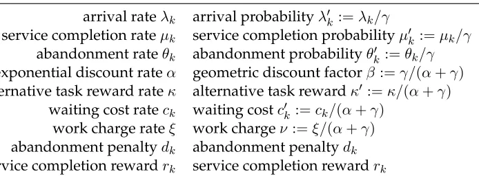
Scenario 1. (Figure 1) In this scenario the WI andcµ/θrules are optimal and the performance of the 2U rule is equivalent except for small values ofθ1. The performance ofcµis good only for
lower values ofθ1, and the difference with respect to WI andcµ/θis the switching point where the
other policies start to serve class-2 customers whilecµdoes not, which makes its suboptimality grow.
Scenario 2. (Figure 2) Because of class-2 high abandonment rates, it is never optimal to serve class 2 and it is optimal to serve class 1 only for lower values of θ1. The 2U and WI policies
capture this feature and are optimal. Thecµ-rule always gives priority to class2, while thecµ/θ -rule correctly prioritizes class1for lower values ofθ1, but then switches to class2, which leads to
[image:17.612.191.395.216.339.2]0 0.5 1 1.5 2 2.5 3 0%
10% 20% 30%
d1
Relative suboptimality gap
[image:18.612.191.395.44.168.2]WI cµ/θ cµ 2U Myopic
Figure 3: Relative suboptimality gap in Scenario 3.
0 2 4 6 8 10
0% 10% 20% 30% 40%
d1
Relative suboptimality gap
WI cµ/θ cµ 2U Myopic
Figure 4: Relative suboptimality gap in Scenario 4.
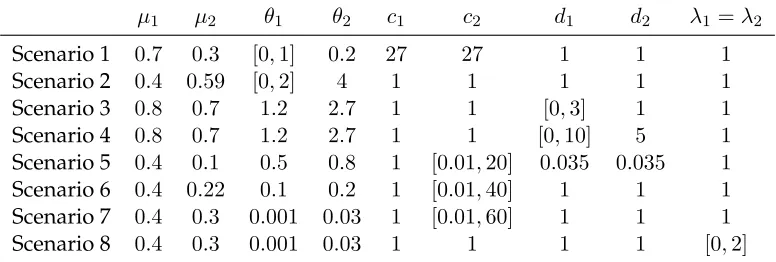
Scenario 3. (Figure 3) For values ofd1smaller than approximately0.42, the optimal policy does
not serve any customer, which is captured by WI and 2U. The other policies however perform dramatically worse. For larger values it is optimal to serve class1customers (or to idle if no class
1customer is present). All the policies give priority to class1, with the only difference being that WI and 2U idle if there is no class1customer, whereascµandcµ/θserve class2in such a case.
Scenario 4. (Figure 4) Though the only difference between this scenario and the previous one is that the value of d2 is now 5 instead of 1, there is a significant difference in the results. Even
though theθ’s are still larger than theµ’s, in this case the performance of 2U and WI differ during a non-negligible range of values ford1. The optimal policy is to serve class 2 and then switch to
serve class 1. The cµ-rule always serves class 1, the Myopic rule always serves class2, and the other policies start serving class2(as a consequence of highd2), and switch to serve class1(first
WI together withcµ/θ, and afterwards 2U) as the value ofd1grows.
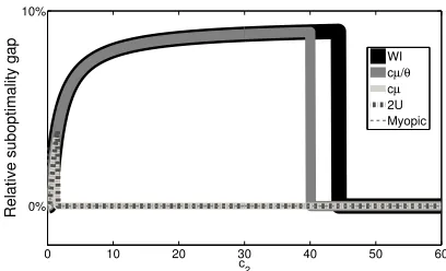
Scenario 5. (Figure 5) The optimal policy is to idle. Policies WI and 2U give priority to idling. The policies cµ and cµ/θ for small values of c2 serve class 1. As the value ofc2 increases, the
policiescµandcµ/θswitch to give priority to class2, what makes a sudden increase in the cost function. The performance of WI and 2U is optimal. The key difference is that WI depends on the differenceµ2−θ2(which is negative), and thanks to this it chooses not to serve class2regardless
[image:18.612.191.396.217.338.2]0 5 10 15 20 0%
10% 20% 30% 40% 50% 60% 70%
c2
Relative suboptimality gap
[image:19.612.192.395.44.170.2]WI cµ/θ cµ 2U Myopic
Figure 5: Relative suboptimality gap in Scenario 5.
0 5 10 15 20 25 30 35 40
0% 10% 20% 30% 40%
c2
Relative suboptimality gap
WI
cµ/θ
cµ
2U Myopic
Figure 6: Relative suboptimality gap in Scenario 6.
Scenario 6. (Figure 6) This is a particularly interesting scenario. Service rates are larger than abandonment rates, and the policy WI has again better performance than the other policies. In fact, WI is optimal for all values ofc2with the exception of a small range around32. The optimal
policy starts serving class1in almost all joint states, but it starts serving class2in more joint states as the value ofc2increases. The WI policy serves class1with strict priority for values ofc2smaller
than32, and class2from that moment on. The upward jump for the other indices happens when they start giving priority to class 2 (firstcµswitches, thencµ/θand then 2U).
The following two scenarios illustrate some specific and uncommon phenomena we have found in our experiments.
Scenario 7. (Figure 7) In this scenario the abandonment rate is very small, say negligible. We recall that without abandonment, the cµ-rule is optimal (Cox and Smith 1961, Buyukkoc et al. 1985). In the numerical experiments we see that, with a rather surprising exception for c2 = 1,
thecµ-rule is indeed optimal in this case and the 2U rule is equivalent tocµ. Policies WI andcµ/θ
start serving class1, and switch later on to class2when the value ofc2becomes sufficiently large.
We emphasize that this is the only scenario we have found where the decision pattern of 2U and WI differs completely and also the only one in whichcµ/θoutperforms WI (for values ofc2
between40and44).
[image:19.612.191.396.216.338.2]0 10 20 30 40 50 60 0%
10%
c2
Relative suboptimality gap
WI
cµ/θ
cµ
[image:20.612.191.395.43.167.2]2U Myopic
Figure 7: Relative suboptimality gap in Scenario 7.
0 0.5 1 1.5 2
0% 10% 20% 30% 40% 50% 60% 70% 80% 90% 100%
λ
1 & λ2
Relative suboptimality gap
WI
cµ/θ
cµ
[image:20.612.188.396.215.334.2]2U Myopic
Figure 8: Relative suboptimality gap in Scenario 8.
a scenario, in which all the rules are optimal in underload, but suboptimal in overload, which is in contrast with, e.g., the results of asymptotic optimality ofcµ/θ.
This scenario is in underload at the beginning and becomes overloaded asλ1andλ2grow.
The optimal policy is to give priority to class1and then switch to class2in some joint states. The Myopic rule always serves class2and all the other rules always serve class1. This scenario thus illustrates that the arrival rates should be taken into account for optimal scheduling, though it is very uncommon to observe such a huge effect.
6.3 Single-server Non-idling System
In this case we do not allow the system to idle, that is, if there are customers in the system, the scheduler must necessarily select one to serve. The policiescµ,cµ/θand Myopic have the same priorities as before, but the optimal policy, the worst-case policy and the WI and 2U rule may behave differently.
We have performed numerical experiments for the same scenarios as in the idling case (see
Table 2). The qualitative performance of the policies is analogous, but whenever there is subopti-mality of any policy, it is in general higher than in the idling case. To illustrate this we discuss the results obtained for Scenarios 2 and 5. In these two scenarios it was optimal to idle in the idling system, which is not allowed now.
Non-idling Scenario 2. (Figure 9) The WI rule is no longer optimal for larger values ofθ1, since
non-0 0.5 1 1.5 2 0%
10% 20% 30%
θ1
Relative suboptimality gap
[image:21.612.192.394.44.168.2]WI cµ/θ cµ 2U Myopic
Figure 9: Relative suboptimality gap in non-idling Scenario 2.
0 5 10 15 20
0% 10% 20% 30% 40% 50% 60%
c2
Relative suboptimality gap
WI
cµ/θ
cµ
2U Myopic
Figure 10: Relative suboptimality gap in non-idling Scenario 5.
negligible interval the WI rule is better than or equivalent to thecµ,cµ/θand Myopic rules. When its performance is inferior to the other policies, the suboptimality in absolute terms is small.
Non-idling Scenario 5. (Figure 10) WI and 2U are no longer optimal for a small interval ofc2
values, but they still outperform the cµ/θ, cµ and Myopic rule, because they do not switch to prioritize class2, while all the other policies do.
6.4 Multi-server Idling System
In order to study the Whittle index rule in the multi-server case, we evaluate the performance of all the rules and the optimal policy for2servers. We believe that this sheds light on the expected performance of these rules even for more servers. Due to the curse of dimensionality we have not evaluated the optimal policy for more servers.
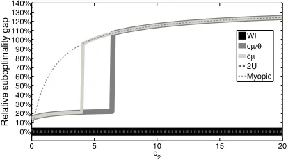
We investigated the same scenarios (seeTable 2) as previously. Performance of the rules in the two-server case is very similar qualitatively to the single-server system. The WI rule is again almost always optimal, and the eventual suboptimality is small. However, the main difference is that the relative suboptimality gap of the other rules becomes more severe. We illustrate this inFigure 11for Scenario2and inFigure 12for Scenario5, where the relative suboptimality gap approximately doubled.
[image:21.612.192.395.217.340.2]0 0.5 1 1.5 2 0%
10% 20% 30% 40% 50% 60% 70% 80% 90% 100%
θ1
Relative suboptimality gap
[image:22.612.191.395.44.159.2]WI cµ/θ cµ 2U Myopic
Figure 11: Multi-server relative suboptimality gap in idling Scenario 2.
0 5 10 15 20
0% 10% 20% 30% 40% 50% 60% 70% 80% 90% 100% 110% 120% 130% 140%
c 2
Relative suboptimality gap
WI cµ/θ
cµ
2U Myopic
Figure 12: Multi-server relative suboptimality gap in idling Scenario 5.
7
Conclusion
We have investigated the problem of scheduling of customers with abandonment. We have pro-posed a comprehensive model accounting for completion rewards, linear waiting costs and aban-donment penalties. For the problem with one or two customers in the system, we have obtained an optimal solution, which is not in the form of an index rule. For the more general case with multiple customers, we have applied Whittle’s relaxation methodology to derive the WI rule, a heuristic scheduling rule which has a very simple structure.
Numerical experiments indicate that WI performs exceptionally well: it is often optimal, and if not, then its suboptimality is small. They also show that in most cases the WI rule out-performs the alternativecµ/θ andcµrules. This is a robust result, that holds in both idling and non-idling systems, independently of system overload conditions, and for the vast majority of scenarios that we have tested. The biggest improvement of WI over cµ/θ and cµ is achieved when it is sometimes optimal to idle, for instance when the abandonment rate is large relative to the service rate. In this case WI may be optimal while the cµ/θcan be performing as the worst policy. Important differences can also be observed when the waiting costs differ across classes. Interestingly, our scheduling rule is well-grounded, as it recovers known optimal policies in some special cases of the problem. For instance, our rule becomes thecµ-rule if there is no abandon-ment. In many cases the performance of 2U is comparable to the performance of WI, however, 2U cannot be easily extended to more than two classes because it is not a simple index rule.
The performance advantage of the WI rule over thecµ/θ rule is primarily due to the fact that the WI rule is designed for our model, where waiting costs are paid while customers are in service as well as in queue, and abandonment does not occur during service, whereas the cµ/θ
[image:22.612.190.397.205.320.2]suggests that much care is needed in appropriately modeling and defining the objective function for a particular system.
An important question for future research is to determine under what conditions the WI rule is optimal or asymptotically optimal. Based on our numerical experiments, we believe that if the WI index values are sufficiently different across classes, then the WI rule is optimal.
The multi-class and/or multi-server problem is much more complex and time- and memory-consuming to simulate due to the curse of dimensionality. We believe that the performance of the WI rule should improve with the number of servers, as suggested by the asymptotic optimality of cµ/θ in overloaded multi-server systems. Moreover, the Whittle and Lagrangian relaxations apply to the multi-server case as well, and the Whittle index rule was shown to be asymptotically optimal when the number of servers grows (under certain technical conditions not satisfied by our model) inWeber and Weiss(1990).
The WI rule is likely to be generalizable to other distributions of service and abandonment, and non-linear waiting costs. The WI index can be interpreted as the expected profit rate, since it is given as the ratio of the expected total profit and the expected service time (or the expected abandonment time).
Acknowledgements
Research partially supported by the French “Agence Nationale de la Recherche (ANR)” through the project ANR JCJC RACON.
References
Aksin, Z., Armony, M., and Mehrotra, V. (2007). The modern call center: A multi-disciplinary perspective on operations management research. Production and Operations Management, 16(6):665–688.
Argon, N., Ziya, S., and Righter, R. (2010). Scheduling impatient jobs in a clearing system with insights on patient triage in mass-casualty incidents. Probability in the Engineering and Informational Sciences, 22(3):301–332.
Ata, B. and Tongarlak, M. H. (2013). On scheduling a multiclass queue with abandonments under general delay costs. Queueing Systems, 74(1):65–104.
Atar, R., Giat, C., and Shimkin, N. (2010). The cµ/θ rule for many-server queues with abandonment.
Operation Research, 58(5):1427–1439.
Atar, R., Giat, C., and Shimkin, N. (2011). On the asymptotic optimality of the cµ/θrule under ergodic cost.Queueing Systems, 67(2):127–144.
Ayesta, U., Jacko, P., and Novak, V. (2011). A nearly-optimal index rule for scheduling of users with abandonment. InIEEE Infocom 2011.
Baccelli, F., Boyer, P., and Hebuterne, G. (1984). Single-server queues with impatient customers. Advances in Applied Prabability, 16:887–905.
Boots, N. and Tijms, H. (1999). A multiserver queueing system with impatient customers. Management Science, 45(3):444–448.
Boxma, O. and de Waal, P. (1994). Multiserver queues with impatient customers. InIn Proceedings of ITC-14, pages 743–756.
Brandt, A. and Brandt, M. (2004). On the two-class M/M/1 system under preemptive resume and impa-tience of the prioritized customers.Queueing Systems, 47:147–168.
Brill, P. and Posner, M. (1977). Level crossings in point processes applied to queues: single-server case.
Buttazzo, G. C. (2011). Hard real-time computing systems: predictable scheduling algorithms and applications, volume 24 ofReal-time Systems. Springer, third edition.
Buyukkoc, C., Varaya, P., and Walrand, J. (1985). Thecµrule revisited. Adv. Appl. Prob., 17:237–238. Cox, D. R. and Smith, W. L. (1961). Queues. Methuen & Co.
Dai, J. and He, S. (2012). Many-server queues with customer abandonment: A survey of diffusion and fluid approximations. Journal of Systems Science and Systems Engineering, 21:1–36.
Down, D., Koole, G., and Lewis, M. (2011). Dynamic control of a single server system with abandonments.
Queueing Systems, 67:63–90.
Fife, D. (1965). Scheduling with random arrivals and linear loss functions. Management Science, 11(3):429– 437.
Gans, N., Koole, G., and Mandelbaum, A. (2003). Telephone call centers: Tutorial, review, and research prospects. Manufacturing & Service Operations Management, 5(2):79–141.
Gittins, J. (1989). Multi-armed Bandit Allocation Indices. Wiley, Chichester.
Gittins, J. and Jones, D. (1974). A dynamic allocation index for the sequential design of experiments. In Gani, J., editor,Progress in Statistics, pages 241–266. North-Holland.
Glazebrook, K., Ansell, P., Dunn, R., and Lumley, R. (2004). On the optimal allocation of service to impa-tient tasks.Journal of Applied Probability, 41(1):51–72.
Graves, S. (1984). The application of queueing theory to continuous perishable inventory systems.
Man-agement Science, 28:401–406.
Harrison, J. M. and Zeevi, A. (2004). Dynamic scheduling of a multiclass queue in the Halfin-Whitt heavy traffic regime. Operations Research, 52(2):243–257.
Hasenbein, J. and Perry(Eds), D. (2013). Special issue on queueing systems with abandonments. Queueng
Systems, 75(2–4):111–384.
Hassin, R. and Haviv, M. (2003).To Queue or not to Queue: Equilibrium Behavior in Queueing Systems. Kluwer Academic Publishers, Boston etc.
Iravani, F. and Balcio ˘glu, B. (2008). On priority queues with impatient customers. Queueing Systems, 58:239–260.
Jacko, P. (2009). Adaptive greedy rules for dynamic and stochastic resource capacity allocation problems.
Medium for Econometric Applications, 17(4):10–16.
Jouini, O., Pot, A., Koole, G., and Dallery, Y. (2010). Online scheduling policies for multiclass call centers with impatient customers. European Journal of Operational Research, 207(1):258–268.
Meilijson, I. and Weiss, G. (1977). Multiple feedback at a single server station. Stochastic Processes and Applications, 5:195–205.
Ni ˜no-Mora, J. (2007). Dynamic priority allocation via restless bandit marginal productivity indices. TOP, 15(2):161–198.
Papadimitriou, C. and Tsitsiklis, J. (1999). The complexity of optimal queueing network. Mathematics of
Operations Research, 24(2):293–305.
Puterman, M. L. (2005). Markov Decision Processes: Discrete Stochastic Dynamic Programming. John Wiley & Sons.
Sevcik, K. (1974). Scheduling for minimum total loss using service time distributions. Journal of the ACM, 21:66–75.
Smith, W. (1956). Various optimizers for single stage production. Naval Res. Logist. Quart., 3:59–66.
Weber, R. and Weiss, G. (1990). On an index policy for restless bandits. Journal of Applied Probability, (27):637–648.
Whitt, W. (2004). Efficiency-driven heavy-traffic approximations for many-server queues with abandon-ments. Management Science, 50:1449–1461.
Whittle, P. (1981). Arm-acquiring bandits.Annals of Probability, 9(2):284–292.
A
Proof of
Proposition 2
Proof. It is straightforward to obtain that the expected total revenue if serving the customer always equals
− c
0
k 1−β+βµ0k,
and that the expected total revenue if not serving her at all equals
−c
0
k+βdkθ0k 1−β+βθk0 .
By taking the difference and rearranging we obtain
c0k
1−β+βθ0k +
βdkθ0k 1−β+βθ0k −
c0k
1−β+βµ0k,
which can be further rewritten as
βc
0
k(µ0k−θk0) +dkθk0(1−β+βµ0k) (1−β+βθk0)(1−β+βµ0k) =Ck.
B
Proof of
Proposition 3
Proof. There are only two possible states of the system: (0)meaning that the system is empty, and (1), meaning that the customer is in the system. For this particular case, from (2) we get
V(0) = 0, and
V(1) = max{ −c01+β(1−µ01)V(1);
−c01−βd1θ10 +β(1−θ01)V(1)},
where the first term refers to serving the customer, and the second term to serve the alternative task. It follows that serving the customer is better than or equivalent to serving the alternative task if and only if
−V(1)(µ01−θ01) +d1θ01≥0. (19)
We solve the Bellman equation and evaluate the value function assuming that serving the customer is optimal, and we get
V(1) = −c
0 1
1−β+βµ01. (20)
Substituting (20) into (19) yields (i).
Claim (ii) is obtained analogously. The only difference is that now serving the alternative task is optimal, and thus the value function is equal to:
V(1) = −c
0
1−βd1θ10
1−β+βθ10 .
C
Proof of
Proposition 4
Proof. Sinceκ0 = −∞, it will never be optimal to engage the alternative task (as long as there is at least one customer in the system), and thus it will have no effect on the characterization of the optimal policy. Further, we can assume that the problem is over once the system is empty, i.e.
V(0,0) = 0. Since there are two customers, equation (2) becomes
V(1,1) = max{−c01−c02+µ01V(0,1) +θ02(−d2+V(1,0))
+ (1−µ01−θ02)V(1,1);
−c01−c02+θ01(−d1+V(0,1)) +µ02V(1,0)
+ (1−θ01−µ02)V(1,1)}
(21)
In states in which there is only one customer present, that is (1,0)and(0,1), the optimal action is to serve the customer present because the alternative task rewardκ0 =−∞andCk ≥0.
From Bellman’s equation we directly obtain that V(1,0) = −c01/µ01 andV(0,1) = −c02/µ02, as in the proof ofProposition 3. Substituting these equalities in the above expression we get
0 =−c01−c02+ max
−µ01c
0 2
µ02 −θ
0 2
d2+
c01 µ01
−(µ01+θ02)V(1,1);
−θ01
d1+
c02 µ02
−µ02c
0 1
µ01
−(θ01+µ02)V(1,1)}
When serving customer 1 is optimal, then the first term within the brackets is equal to the left-hand side and greater than or equal to the second term. It is straightforward to obtain that this is equivalent to
c01(µ01−θ10) +d1θ10µ01
µ01(θ10 +µ02) ≥
c02(µ02−θ20) +d02θ02µ02 µ02(θ02+µ01) .
We have thus obtained that the index value νk2U given in (6) characterizes which customer it is
optimal to serve.
D
Proof of
Theorem 1
Proof. The proof of this theorem is based on establishing indexability of the problem and comput-ing the index values followcomput-ing the survey Ni ˜no-Mora(2007). We will rewrite our minimization problem as a maximization one. Indexability is in fact equivalent to existence of the quantities with stated properties, and is valid because any binary-state MDP is indexable.
Let us denote the optimal value function by Vk,n for customerk in staten. The Bellman
equation for state1and customerk∈ K, after plugging in the definitions of the action-dependent parameters for a state becomes:
Vk,1 = max{Rk,11−νWk,11+β[µ 0
kVk,0+ (1−µ0k)Vk,1];
After plugging in the formulas for expected one-period revenues and expected one-period capacity consumption, we obtain:
Vk,1 = max{ −c0k−ν+β[µk0Vk,0+ (1−µ0k)Vk,1]; (22)
−c0k−βdkθ0k+β[θ
0
kVk,0+ (1−θ0k)Vk,1]},
where the first term in the curly brackets corresponds to serving and the second term corresponds to not serving the customer. Note that the Bellman equation forVk,0is:
Vk,0 = max{R1k,0−νWk,10+βVk,0;R0k,0−νWk,00+βVk,0}
= max{−ν+βVk,0;βVk,0}.
Forν ≥0, it is straightforward to obtain thatVk,0= 0. Analogously forν <0we obtain:
Vk,0 =−
ν
1−β.
Statement (ii) follows immediately. Next we prove (i), dividing the proof into two cases.
Case ν ≥ 0 In statement (i), we want to show when it is optimal and when it is not optimal to serve waiting customerk. We derive the value ofVk,1. When we choose to serve the customer, we
get:
Vk,1 =−c0k−ν+β[µ
0
kVk,0+ (1−µ0k)Vk,1],
and it is straightforward to obtain:
Vk,1 =−
c0k+ν
1−β+βµ0k.
We substitute the expressionsVk,0 andVk,1 in (22) to obtain, after rearranging, a condition
for serving customerk:
βc
0
k(µ
0
k−θ
0
k) +dkθ0k(1−β+βµ
0
k) 1−β+βkθ0k
≥ν.
Sinceν≥0, this is equivalent toνk,1≥ν.
Analogously to above we can show that if it is optimal not to serve waiting customerk, then
νk,1 ≤ν.
Case ν < 0 We can similarly prove that statement (i) also holds ifν < 0. All the steps will be similar, but note that we now haveVk,0 =−1−νβ.
If serving is optimal, from equation (22),we have
Vk,1=
−c0k−ν−βµ0k1−νβ
1−β+βµ0k . (23)
We next substitute the expressions of Vk,0 and Vk,1 in the equation (22). We want to derive a
condition to determine when it is optimal to serve. I.e., when the first term in (22) is greater or equal to the second. After rearranging, we obtain:
ν ≤βc
0