A Method for Solving Fuzzy Partial Differential Equation by Fuzzy Separation Variable

(1)

© 2019, IRJET | Impact Factor value: 7.211 | ISO 9001:2008 Certified Journal

| Page 77

A METHOD FOR SOLVING FUZZY PARTIAL DIFFERENTIAL EQUATION BY

FUZZY SEPARATION VARIABLE

Jeyavel Prakash

1

_{, Ramadoss ArunBalaji}

2

_{, Dereje wakgari}

2

1

_{Department of Mathematics, Srinivasa Ramanujan Centre, SASTRA Deemed University, Kumbakonam, India.}

2

_{College of Natural and computational sciences, WOLLEGA University, Nekemte, ETP.}

*---***---*

ABSTRACT: - In this paper a numerical method for solving fuzzy transport equation is considered and also we use separable variable method to solve fuzzy transport equation. First described the preliminaries definitions, and then consider a finite difference scheme for the one dimensional transport equation, then described the fuzzy separation variable method. We use Matlab for numerical calculation. In this example, it obtains the Hausdorff distance between Finite different scheme solution and separable variable solution.

KEYWORDS:

Fuzzy number, Fuzzy transport equation, Finite different scheme, Stability, Fuzzy separable variable

INTRODUCTION:

Fuzzy differential equations have been applied extensively in recent years to model uncertainty in mathematical models. Fuzzy transport equation is one of the simplest Fuzzy partial differential equation, which may appear in many applications. The concept of a fuzzy derivative was first introduced by Chang and Zadeh [8] and others. Fuzzy differential equations were first formulated by Kaleva [9] and Seikkala [10] in time dependent form. Kaleval had formulated fuzzy differential equations, in term of derivative [9]. Buckley and Feuring have given a very general formulation of a fuzzy first-order initial value problem. They first find the crisp solution, fuzzify it and then check to see if it satisfies the FDE. Furthermore, some numerical methods for solving FDE are discussed in [11, 12, 13, and 14].

In this paper, using Fuzzy separation variable method and finite different scheme procedure are presented. The paper has been organized as follows. In first section described some basic definitions of fuzzy set and fuzzy number which have been discussed by L.A. Zadeh. Then described with finite difference scheme and implemented on transport equation. The necessary condition for stability of proposed method will discussed following section. Introduced Fuzzy separable variable method for fuzzy transport equation is discussed in next section. Example and solution of results are presented in later section. The paper concludes with a section on conclusion.

PRELIMINARIES

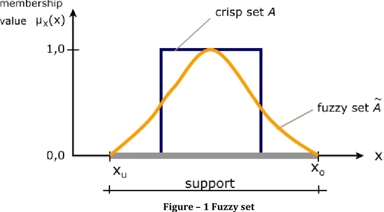
Classical sets are also called ‘crisp’ sets so as to distinguish them from fuzzy sets. In fact, the crisp sets can be taken as special cases of fuzzy sets. Let A be a crisp set defined over the universe X. Then for any element x in X, either x is a member of A or not. In fuzzy set theory, this property is generalized. Therefore, in a fuzzy set, it is not necessary that x is a full member of the set or not a member. It can be a partial member of the sets. The generalization is performed as follows: For any crisp set A it is possible to define a characteristic function , the characteristic function takes either of the values 0 or 1 in the classical set, for a fuzzy set, the characteristic function can take any value between zero and one [1].

Definition:

The membership function ̃ of a fuzzy set ̃ is a function ̃: X  [0, 1]

So every element in x in X has membership degree [7]: ̃

(2)

© 2019, IRJET | Impact Factor value: 7.211 | ISO 9001:2008 Certified Journal

| Page 78

Definition:

The set of elements that belong to the fuzzy set ̃ at least to the degree is called the – cut set: ̃ (2)

̃ is called strong - cut[1].

Figure – 1 Fuzzy set

Definition:

[image:2.612.120.495.157.364.2]

The triangular fuzzy number ̃ is defined by three numbers as follows, ̃ = This representation is interpreted as membership function [1] (Fig.1)

Figure – 2 Fuzzy Numbers

̃

{

}

(3)

If ̃ ( ̃ )

(3)

© 2019, IRJET | Impact Factor value: 7.211 | ISO 9001:2008 Certified Journal

| Page 79

We represent an arbitrary fuzzy number by an ordered pair of function( ), which satisfies the following requirements:[2]

1. is a bounded left continuous non decreasing function over [0,1].

2. is a bounded right continuous non increasing function over [0,1].

3. , . Where are crisp numbers

For arbitrary fuzzy number x = ( ) , y = and real number k :

1. X = y if and only if for all .

2. Kx = {( )

( ) }

3. x + y = ( ) 4. x – y = ( )

5. x.y = { { } { }}

Since the - cut of fuzzy numbers are always a closed and bounded, interval, so we can write ̃ [ ], for all

The Hausdorff metric DH is defined by

DH(u, v) = {| | } (4)

This metric is a bound for error. By it we obtain the difference between exact solution and approximate solution. FINITE DIFFERENCE METHOD: Assume ̃ is a fuzzy function of the independent crisp variable x and t. Subdivided the x – t plane into sets of equal rectangles of sides by equally space grid lines parallel to Oy, defined by xi = ih, i = 0,1,2,3 …. And equally spaced grid lines parallel to Ox, defined by yj = jk , j = 0,1,2,…. Denote the value of ̃ at the representative mesh point p(ih, jk) by [11, 12, ] ̃p = ̃ ̃I,j (5) And also denote the parametric form of fuzzy number, ̃I,j as follow ̃i,j = ( ) (6)

We have (Dt) ̃i,j = ( ) (7)

(Dx) ̃i,j = ( ) (8)

(DxDx) ̃I,j = ( ̃ ̃ ) (9)

(4)

© 2019, IRJET | Impact Factor value: 7.211 | ISO 9001:2008 Certified Journal

| Page 80

(13)

And also (Dx) ̃i,j at p we have

(14)

̃

₍₁₅₎

Now consider one dimensional transport equation (Dt) ̃i,j = ( ̃ Dxx- ̃ Dx) ̃i,j (16)

Where, ̃ is fuzzy coefficient of diffusion, ̃ fuzzy coefficient of convection and ̃i,j critical fuzzy chloride concentration

depassive the reinforcement.

That the have continuous partial differential, therefore (Dt) ̃i,j = ( ̃ Dxx - ̃ Dx) ̃i,j

Parametric form of Transport equation is

̃ ( ̃ ) ̃ ( ̃ ) (17)

̃ ( ̃ ) ̃ ( ̃ ) (18)

By (9),(10),(11),(12),(13) and (14) the different scheme for transport equation is,

̃ ( ) ̃ ( )

_̃ ₍ _{) ̃ (} ₎

Or the following equation must be hold

(19)

(20)

Where ̃i,j = ( ) is the exact solution of the approximating difference equations, xi = ih,

(i = 0,1,2,3 ….n) and yj = jk , (j = 0,1,2,….n), r1 = ̃ and r2 = ̃ . (21)

A necessary condition for stability:

Consider the stability of the classical implicit equation. If the boundary values are know at i = 0 and N,

j >0, then the 2(N-1) equations can be written in matrix as

(

)₍

) (

(5)

© 2019, IRJET | Impact Factor value: 7.211 | ISO 9001:2008 Certified Journal

| Page 81

A(

) ( ) (

) ₍ _{) (|A} ₍₂₂₎

Where

A = (

), E =



















0 ...

...

)

(r

0 ...

)

(r

0

1 1 2 1 1 2

r

, F =

                  ) 2 1 ( ... ... ) 2 1 ( ... ) 2 1 ( 1 2 1 2 1 2 r r r r r r Definition:

Let matrix A has special structure as follow( ). Then the eigenvalues of A are union of eigenvalues of E+F and eigenvalues of E-F [3].

Definition: The largest of the eigenvalues of matrix A, is showed by

Definition:The necessary and sufficient condition for the difference equations to be stable is

[4] (23)

Remark (1): If A-1_{be inverse of matrix A, then}

[5]. (24)

Remark (2): The eigenvalues of a N x N tridiagonal matrix













a

c

b

a

c

b

a

c

b

a

...

are √ , s = 1, … N [4] (25)

Kellogg Lemma[6]:

Let r > 0, and G is nonnegative definite real matrix, then

{

} (26)

Theorem:

Let matrix A has special structure as follow(

). Then the eigenvalues of A are union of eigenvalues of E+F and

eigenvalues of E-F

(6)

© 2019, IRJET | Impact Factor value: 7.211 | ISO 9001:2008 Certified Journal

| Page 82

Where,S1 =E + F =





























1 2 1 1 2 1 2 1 1 2 1 2 1 1 2 1 2

2

1 )

(

2

1 ...

...

)

(

2

1 )

(

2

1 r

r

and S2=E – F =















































1 2 1 1 2 1 2 1 1 2 1 2 1 1 2 1 2

2

1 )

(

2

1 ...

...

)

(

2

1 )

(

2

1 r

r

By equation (26),

√

(

r

₂



r

₁

)

, K = 1, 2… N-1.

√

(

r

₂



r

₁

)

, K = 1, 2… N-1.

We know ₍ _√

₍

₎

1

2

r



(27)

Our assumption of r1 and r2 are not equal to zero and r2 should be greater that r1, that’s r2 – r1 should be nonnegative and Max

| = 1

( √

(

r

2



r

1

)

By Kellogg lemma

_√

₍

₎

1 2

r



< 1 for all r1,r2 >0 (28)

Therefore our difference scheme is unconditionally stable.

FUZZY SEPARATION OF VARIABLE:

In developing a solution to a Fuzzy partial differential equation (FPDE) by Fuzzy separation of variables, one assumes that it is possible to separate the contributions of the fuzzy independent variables into Fuzzy separate functions that each involves only one fuzzy independent variable. The method of Fuzzy separation of variables must be working with fuzzy linear homogenous partial differential equations with fuzzy linear homogeneous boundary conditions. At this point are going to worry about the initial conditions because the solution that we initially get will rarely satisfy the initial conditions. The method of Fuzzy separation of variables relies upon the assumption that a function of the form,

(7)

| Page 83

Where ̃ a fuzzy is function of x and ̃ is a fuzzy function of t. The fuzzy functions are simple because any temperature ̃ of this form will retain its basic “shape” for different value of time t. The general idea is that it is possible to find an infinite number of these solutions to the FPDE. These simple fuzzy functions

̃ ̃ ̃ (30)

The solution ̃ , they are looking for is found by adding the simple fundamental solution ̃ ̃ in such a way that the resulting sum

∑ ̃ ̃ ̃ (31)

will be a solution to a Fuzzy linear homogeneous partial differential equation in . This is called fuzzy product solution and provided the boundary conditions are also fuzzy linear and homogeneous this will also satisfy the boundary conditions.In order to use the method of fuzzy separation of variables, if would be working with a fuzzy linear homogenous partial differential equation with fuzzy linear boundary condition. At the point of initial conditions are not worried, because the solution that initially get will rarely satisfy the initial conditions. However there are ways to generate a solution that will satisfy initial condition provided they meet some fairly simple requirements.

Consider the fuzzy transport equation

̃

̃ ̃ ̃

̃

, 0<x<1, t >0 (32)

̃ ̃ ̃ ̃

Given PDE is ̃ ̃ ̃

̃ ̃

, 0<x<1, t >0

Let ̃ ̃ ̃

̃ ̃ ̃ , ̃ ̃ ̃ and ̃ ̃ ̃

Substituting the given PDE is

̃ ̃ ̃ ̃ _{̃ ̃ ̃}_̃

̃ ̃

̃ ̃ ̃ ̃ ̃

Since L.H.S is a function of x only, R.H.S is a function of t only, it must have

̃ ̃ ̃,

̃ ̃ _{̃ ̃}

̃ ̃ and ̃ ̃

Assume that are interested ̃ valid for all t.

Case (I): If ̃ , So in this case the only solution is the trivial solution and so is not an eigenvalue for this boundary value problem.

Case (II): If ̃

Let ̃ ̃

That implies ̃ ̃ ̃ and ̃ ̃ _{̃ ̃} _̃ _̃

̃ ̃ ̃ ; ̃ ̃ ̃ ̃

(8)

| Page 84

̃ ̃ ̃ _̃̃ _{, where ̃} ̃ ̃

√ ̃ ̃ ̃

and ̃ ̃

√ ̃ ̃ ̃

̃  ̃ ̃

Case (III): If ̃

Let ̃ ̃

That implies ̃ ̃ ̃ and ̃ ̃ _{̃ ̃} _̃ _̃

̃ ̃ ̃ ;

This is simple linear (and separable for that matter) first order differential equation,

̃ ̃ ̃ ̃

We known that ̃ ̃ , that is

̃ ̃ _{̃ ( ̃ )}_{̃ ( ̃ ) , where ̃} ̃

̃ and

√ ̃ ̃ _̃

̃  ̃

̃  ( ̃ ) ( ̃ ) , N = 1,2,3,…

̃

The positive eigenvalues and their corresponding eigenfunctions of this boundary value problem are then,

̃

̃ ̃̃ ̃ ( ₎

̃ ̃ ̃

Our product solution is,

̃ ̃ ( ) ( ) ̃ ( ̃ ̃)

Note however that fact found infinitely many solutions since there are infinitely many solutions (i.e. eigenfunctions) to the spatial problem. Since the linear combination of particular solution is also a solution, we have

̃ ∑ ̃ ( ) ( ) ̃ ( ̃

̃) _{N = 1, 2, 3, … (33)}

EXAMPLE:

Consider the fuzzy transport equation

̃

, 0<x<1, t >0

BC ̃ ̃

(9)

| Page 85

SOLUTION:

Now applying for the fuzzy separable variable method to described the solution in equation (33),

̃ ∑ ̃ ( ) ()

That the initial condition ̃ ̃

̃ _{∑ ̃} ()

Expanding the initial temperature ̃ ,

̃ () _{[ ̃}_̃ _̃_]

Multiply on both sides and taking integrate from 0 to 1, then

Note: ∫ {_}

∫ ̃ ̃  ̃

̃ ̃ ( ) () (34)

Consider, ̃ = [

, for

for

( ) ( ) (35)

( ) ( ) (36)

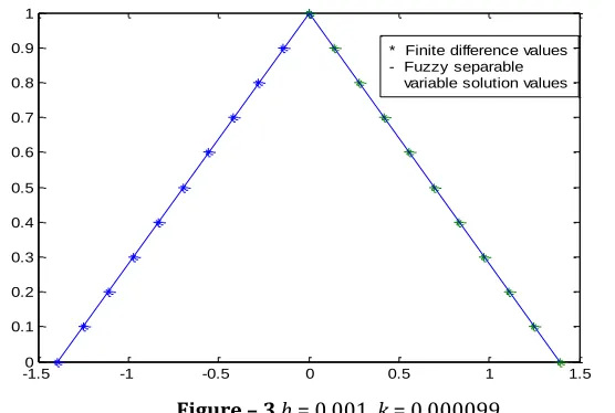
The fuzzy separable variable solution and finite difference solutions are shown in Figure (3) at the point (0.7, 0.005)with h = 0.001, k = 0.000099 .

[image:9.612.171.449.539.726.2]

The Housdorff distance between solutions is 0.001

Figure – 3 h = 0.001, k = 0.000099

-1.50 -1 -0.5 0 0.5 1 1.5

0.1 0.2 0.3 0.4 0.5 0.6 0.7 0.8 0.9 1

(10)

| Page 86

CONCLUSIONS:

The fuzzy partial differential equation can be applied for modeling in physics, engineering and mechanical systems. In this paper introduced fuzzy separable variable method to solve for Transport equation. And also compare with fuzzy separable variable solution and finite difference solution and then described with the Hausdroff distance between fuzzy separable variable solution and finite difference solution, moreover the finite difference method gave a good approximation for the solution.

REFERENCES:

[1]. T J Ross,” Fuzzy logic with engineering applications”, Addison – Wesley, 1985.

[2]. O.Kaleva, “The Cauchy problem for fuzzy differential equations”, Fuzzy sets and systems, 35, 1990.

[3]. T.Allahviranloo, N.Ahmadi, E. Ahmadi, Kh. Shams Alketabi, “Block Jacobi two-stage method for fuzzy systems of linear equations, Applied mathematics and computation 175 (2006) 1217 – 1228”.

[4]. G.D. Smith, “Numerical solution of partial differential equation”, 1993.

[5]. Biswa Nath Data, “Numerical Linear Algebra and applications”.

[6]. B. Kellogg, “An alternating Direction Method for Operator Equations”, J. Soc. Indust. Appl. Math.(SIAM). 12 (1964) 848-854.

[7]. L.A. Zadeh, “The concept of a linguistic variable and its application to approximate reasoning”, inform. Sci. 8 (1975) 199-249.

[8]. S.L Chang, and L.A. Zadeh, “On fuzzy mapping and control”, IEEE, Transactions on systems man and Cybernetics, Vol.2, pp. 30-34, 1972.

[9]. O. Kaleva, “Fuzzy differential equations”, Fuzzy Sets and Systems 24 (1987) 301-317.

[10]. S. Seikkala, “On the fuzzy initial value problem”, Fuzzy Sets and Systems 24 (1987) 319- 330.

[11]. M. Ma, M. Fridman, and A. Kandel, “Numerical solutions of fuzzy differential equations”, Fuzzy Sets and Systems, vol.105, pp.133{138, 1999.

[12]. S.Abbasbandy, T. Allahviranloo, O. Lopez-Pouso, and J.J. Nieto, “Numerical Methods for fuzzy differential inclusions”, J. Computer and mathematics with Applications, vol.48, Pp, 1633-1641, 2004.

[13]. S. Abbasbandy, and T. Allahviranloo, “Numerical solutions of fuzzy differential equations by Taylor method”, J.Computational methods in Applied Mathematics, vol.2, pp.113-124, 2002.