Communication system design and analysis for asynchronous molecular timing channels

Communication System Design and Analysis

for Asynchronous Molecular Timing Channels

Nariman Farsad,

Member, IEEE,

Yonathan Murin,

Member, IEEE,

Weisi Guo,

Senior Member, IEEE,

Chan-Byoung Chae,

Senior Member, IEEE,

Andrew W. Eckford,

Senior Member, IEEE,

and

Andrea Goldsmith,

Fellow, IEEE

Abstract—Two new asynchronous modulation techniques for molecular timing (MT) channels are proposed. One based on modulating information on the time between two consecutive re-leases ofindistinguishableinformation particles, and one based on usingdistinguishable particles. For comparison, we consider the synchronized modulation scheme where information is encoded in the time of release and decoded from the time of arrival of particles. We show that all three modulation techniques result in a system that can be modeled as an additive noise channel, and we derive the expression for the probability density function of the noise. Next, we focus on binary communication and derive the associated optimal detection rules for each modulation. Since the noise associated with these modulations has an infinite variance, geometric power is used as a measure for the noise power, and we derive an expression for the geometric SNR (G-SNR) for each modulation scheme. Numerical evaluations indicate that for these systems the bit error rate (BER) is constant at a given G-SNR, similar to the relation between BER and SNR in additive Gaussian noise channels. We also demonstrate that the asynchronous modulation based on two distinguishableparticles can achieve a BER performance close to the synchronized modulation scheme.

Index Terms—Molecular communication, channel models, noise models, L´evy distribution, stable distributions, bit error rate, and molecular timing channel.

I. INTRODUCTION

M

OLECULAR communication is a biologically inspired form of communication, where chemical signals are used to transfer information [3]–[5]. It is possible to modulate information on the particles using different techniques such as concentration [6], type, ratio [7], number [8], time of release [9], or a combination of these techniques [3]. Moreover, information particles can be transported from the transmitter to the receiver using diffusion [10], active transport [11], bacteria [12], and/or flow (or advection) [13]. Between all these techniques, diffusion and flow-based propagation are the

This work was been presented in part at the 2015 IEEE Global Commu-nications Conference (GLOBECOM’2015) [1], and at the 2016 IEEE Global Communications Conference (GLOBECOM’2016) [2].

N. Farsad, Y. Murin, and A. Goldsmith are with the Department of Electrical Engineering, Stanford University, Stanford, CA, USA, W. Guo is with the School of Engineering, University of Warwick, Coventry, UK. C.-B. Chae is with the School of Integrated Technology, Yonsei University, Korea. A. Eckford is with the Department of Electrical Engineering and Computer Science, York University, Toronto, Canada.

This research was supported in part by the NSF Center for Science of Information (CSoI) under grant CCF-0939370, the NSERC Postdoctoral Fel-lowship fund PDF-471342-2015 and by the Basic Science Research Program (2017R1A1A1A05001439) funded by the MSIP, Korea, through the NRF of Korea.

easiest to implement, and a few experimental platforms have been built to demonstrate molecular communication based on these transport mechanisms [14]–[16].

In this work we focus on modulation techniques for molec-ular communication and their corresponding system models. Most prior work on modulation techniques rely on the con-centration or the type of the released particles. For example in [17], the order of release of consecutive distinguishable particles is proposed for encoding information. In this work, we consider molecular timing (MT) channels where timing-based modulation is employed. Only a few works have con-sidered this type of modulation: In [9] the time of release of the particles is used for encoding information, while in [18] the information is encoded in the time interval between two pulse releases of information particles in mirofluidic channels. The work [19] showed that in the case of timing-based mod-ulation, where information is encoded on the release timing of particles, and the transport mechanism is diffusion assisted by constant laminar flow, the channel can be represented as an additive noise channel. In this case the noise term follows the inverse Gaussian (IG) distribution. Capacity bounds for the additive IG noise channel, in bits per channel use, under an average delay constraint, were derived in [19], [20]. In [1], we have shown that in the case of timing-based modulation, where information is encoded on the release timing of particles, and pure diffusive transport (i.e., diffusion without any flow) is employed, the channel can be represented as an additive noise channel where the noise follows the L´evy distribution. The capacity of this channel was studied in [21]–[24], and it was shown that this capacity can increase poly-logarithmically with respect to the number of simultaneously released particles. A sequence detector for this modulation scheme was presented in [25].

these applications can be designed with great precision [29], [30].

The three systems considered in this paper are as follows. First, we consider a synchronized MT system, where informa-tion is encoded in the release timing of informainforma-tion particles (system A); second, an asynchronous MT system is pro-posed where information is encoded in the time between two consecutive releases ofindistinguishableinformation particles (system B); and finally, another asynchronous MT system is considered where information is encoded in the time between two consecutive releases of distinguishable information par-ticles (system C). Fig. 1 depicts all three systems. One of the main motivations for proposing these new modulations is the challenge of synchronization. In particular, for some applications involving micro and nano-scale devices, it may be difficult to synchronize the transmitter and the receiver due to their small size and limited power. In this case, the modulation scheme in system A, which has been used in previous works, may be too difficult to implement in practice. The newly presented modulation schemes in systems B and C, however, do not require synchronization between the trans-mitter and the receiver. These modulations are analogous to differential phase-shift keying (PSK) in that the asynchronous MT modulations do not require an absolute time reference, while the differential PSK does not require an absolute phase reference.

It must be noted that stable distributed noise arises in system models for a number of different applications. Therefore, the results of this paper could also be applicable in those areas. Specifically, in [31], alpha-stable distributed noise was used to model room acoustics. In radio communications, symmet-ric alpha-stable distributions were used to model impulsive non-Gaussian noise such as those that exists in ultra-wide bandwidth systems [32], [33]. Capacity bounds for a special class of alpha-stable additive noise channels were provided in [34], [35]. Although in this work we focus on additive stable distributed noise channels in the context of molecular timing channels, the analysis and the results are applicable to the general detection problem in additive stable distributed noise channels.

There are only three classes of stable distributions with closed-form probability density functions (PDF) in terms of elementary functions: Gaussian, Cauchy, and L´evy. In this work, we derive closed-form expressions for the PDFs of the noise terms in systems B and C in terms of the complex error function and Voigt functions [36], [37], which are used in other fields of science such as physics. Thus we develop new closed-form PDF results for a subclass of stable noise distributions in terms of the Voigt functions, which can be efficiently calculated numerically [38], [39], and can be approximated using elementary functions in some special cases [40].

To compare the performance of the three proposed modula-tion schemes, we consider a binary communicamodula-tion system and derive the optimal detection rule for each modulation technique. Since the system noise in all three cases is heavy-tailed with infinite variance, the standard definition of signal power, used in electromagnetic communication, is not suitable. Instead, we derive the expressions for the geometric power

[41] of a large class of stable distributions, and use it to represent the noise power. Furthermore, instead of using the well known signal-to-noise ratio (SNR) metric, we use the geometric SNR (G-SNR) [41] metric, which is given by the geometric power of the signal divided by the geometric power of the noise with some normalization constants. Based on numerical evaluations we observe that for the modulations considered, the bit error rate (BER) is constant for a given G-SNR regardless of the geometric signal power and the geometric noise power.

Based on the above derivations, we next use numerical evaluations to compare the BER of all three systems. We show that system B with indistinguishable particles exhibits the highest BER, while system A achieves the lowest BER. This indicates that time-synchronized transmission over MT channels, i.e. Modulation A, works better than the other two modulations considered. We further show that by adjusting the diffusion coefficients of the information particles in system C, which is an asynchronous transmission, the BER can approach the BER of system A, where full synchronization is assumed. However, this comes at the cost of added system complexity where both the transmitter and receiver must be capable of transmitting and detecting two distinguishable particles.

The rest of this paper is organized as follows. In Section II we present the three timing-based modulation techniques, and derive an additive noise system model for each of them. In Section III we focus on the diffusion-based propagation and derive the PDF for the additive noise term for each system. In Section IV, binary communication is studied, and the optimal detectors are derived. The geometric power of the noise and the G-SNR of each system are derived in Section V. Numerical BER evaluations of the proposed modulation techniques are presented in Section VI, and concluding remarks are provided in Section VII.

Notation:We denote the set of real numbers byR, and the

set of positive real numbers by R+_{. Other than these sets,}

we denote sets with calligraphic letters, e.g., T. We denote random variables (RV)s with upper case letters, e.g., X and

Y, and their realizations with the corresponding lower case letters, e.g., x andy. We use fY(y) to denote the PDF of a

continuous RV Y onR,fY|X(y|x)to denote the conditional

PDF ofY givenX, and FY(y)andFY|X(y|x)to denote the

corresponding cumulative distribution functions (CDF). We use ϕX(ω) to denote the characteristic function of the RV X and we use the notation X =d Y to denote the equality in distribution, i.e., X has the same PDF as Y. We use | · | to denote the absolute value,j _,√−1 to denote the imaginary number, and <{z} to denote the real part of the complex numberz. Finally,erfc (·)is used to denote the complementary error function given byerfc(x) = √2

π

R∞

x e

−u2 du.

II. SYSTEMMODELS

Transmitter Particle Generator

Emission/Release Control Information

Particles

Release Time

Tx

Detection & Reception

Receiver

Arrival Time

Ty

Random Propagation

SYSTEM A

Ty = Tx + Tn

Time Between Release

Lx

Time Between Arrivals

Ly

SYSTEM B

Random Propagation

Ly = |Lx + Ln|

Time Between Release

Zx

Time Between Arrivals

Zy

SYSTEM C

Random Propagation

Zy = Zx + Zn

Fig. 1. Summary of the System models corresponding to each modulation scheme. System A: a synchronized MT, system B: an asynchronous MT with indistinguishable information particles, and system C: an asynchronous MT with distinguishable information particles

channel model. To develop our model, we make the following assumptions about the system:

A1) The transmitter perfectly controls the release time of each information particle, and the receiver perfectly measures the arrival times of the information particles. Furthermore, the transmitter and the receiver are perfectly synchronized in time, when synchronization is required by the modulation scheme.

A2) Any information particle that arrives at the receiver is absorbed and hence is removed from the propagation medium.

A3) All information particles propagate independently of each other, and their trajectories are random according to an independent and identically distributed (i.i.d.) random process. This is a fair assumption for many different propagation schemes in molecular communication such as diffusion in dilute solutions, i.e., when the number of particles released is much smaller than the number of molecules of the solutions.

A4) There is no inter-symbol interference (ISI) between con-secutive channel uses.1_{In practice this assumption can be}

satisfied if the time between consecutive channel uses is large enough or if chemical reactions are used to dissipate

1_{In [25] we study communication over DBMT channels in the presence of}

ISI.

the particles [42].

A5) Initially, there are no information particles in the envi-ronment and the particles that arrive at the receiver are the ones released by the transmitter.

Note that these assumptions are typical in the study of molec-ular communication systems [20], [43]–[50].

Moreover, as our system uses molecular timing channels through microfluidic links on bio-chips, the assumptions can be satisfied as follows. In bio-chips, it is possible to release and detect information particles with great precision [29], [30] (satisfies A1). Many detectors will remove the information particles as part of the detection process, e.g., by binding to a receptor, diffusion into a sensing layer, or chemical reactions (satisfies A2). The number of information particles released as part of the modulation techniques considered in this work are one or two (satisfies A3). The applications considered in this work are biological studies, where only a very few bits of information need to be transmitted followed by large periods of silence (satisfies A4). Finally, the microfluidic links can be carefully monitored and designed to exclude interfering molecules (satisfies A5).

The first MT system that we consider is the one proposed in [9], [19], where the information is encoded in the release timing of a single information particle. LetTx∈ T ⊆ R+ be

the release time of the information particle at the transmitter. In this scheme, the information is modulated onto the release time itself. The released particle is then transported from the transmitter to the receiver, where the transport process is random. LetTy be the time of arrival at the receiver. Then we

have

Ty =Tx+Tn, (1)

whereTn is the random propagation delay of the information

particle, which is the noise term in this channel. One of the main challenges of this modulation scheme is the need for synchronization between the transmitter and the receiver. In this work, whenever system A is used we assume that the transmitter and the receiver are perfectly synchronized.

To overcome this synchronization challenge, we propose two new modulation schemes in which information is mod-ulated on the time durationbetween two consecutive releases of information particles. The receiver decodes the information from the time between the arrivals of two molecules. Note that in this case synchronization between the transmitter and the receiver is not required. Two cases are possible: either the two released information particles are indistinguishable

at the receiver, or the two released information particles are

distinguishable at the receiver.

We first consider the case where both information particles are indistinguishable. Without loss of generality, let Tx1 be

the release timing of the first information particle and letTx2

be the release timing for the second information particle, with

Tx2 > Tx1. Thus, the information is encoded in Lx=Tx2− Tx1. Using (1), the system model for this modulation scheme

is given by:

|Ty2−Ty1|=|Tx2−Tx1+Tn2−Tn1|,

[image:3.612.53.293.56.378.2]

whereLn=Tn2−Tn1is the random noise term in this system,

and Tn2 and Tn1 are the random propagation delays for the

first and the second particles as in (1). Note that the absolute value in the system formulation is due to the fact that both information particles are indistinguishable, and therefore the receiver can observe only the absolute difference of arrival times.

The last modulation scheme uses the time between releases of twodistinguishableinformation particles (i.e., two different particle types) to encode information. Let Txa be the release

timing of the type-a information particle and let Txb be the

release timing of the type-b information particle. We assume that the information is encoded inZx=Txb−Txa. Unlike (2)

where Lx is always positive, Zx can be positive or negative

depending on the order that the type-aand type-binformation particles are released. Using (1), the system model for this scheme is given by:

T_yb−T_ya=T_xb−T_xa+T_nb−T_na,

Zy=Zx+Zn, (3)

where Zn = Tnb −Tna is the random additive noise term

in this system, and Tb

n and Tna are the random propagation

delays for the type-a and type-b particles as in (1). Again, no synchronization is required between the transmitter and receiver. Fig. 1 summarizes all three modulation techniques.

Note that the proposed modulation schemes and their corre-sponding system models could be applied to any type of prop-agation model through the medium as long as Assumptions

A1)-A4) are not violated. In the next section, we derive the distribution of the noise terms for the proposed MT systems, when diffusion propagation is used for particle transport.

III. NOISEMODELS FORDBMT SYSTEMS

In the rest of this work we focus on DBMT systems where diffusion is used for particle transport. In particular, in this section we derive the PDF of the noise terms Tn, Ln, and Zn for DBMT systems in (1)-(3), and discuss some of the

properties of these RVs.

A. System A

To specify the random additive noise termTn in system A,

we define a L´evy-distributed RV as follows.

Definition 1 (L´evy Distribution): Let the RV X be L´evy-distributed with location parameter µ and scale parameter c

[28]. Then its PDF is given by:

fX(x;µ, c) =

  

q _c

2π(x−µ)3 exp

− c

2(x−µ)

, x > µ

0, x≤µ

, (4)

its characteristic function is given by:

ϕ(ω;µ, c) = expjµω−p−2jcω, (5)

and its CDF is given by:

FX(x;µ, c) =

  

erfc

q _c

2(x−µ)

, x > µ

0, x≤µ

. (6)

Throughout the paper, we use the notation X ∼L(µ, c) to indicate a L´evy RV with parametersµandc.

Assumption A2) implies that the distribution of Tn is the

distribution of the first hitting time (first arrival at the receiver) of a particle transported via diffusion without flow. In previous works, it was shown that the first hitting time for a diffusion channel with constant drift (i.e., flow) in 1-dimensional space follows the inverse Gaussian distribution [19]. In this work, we consider the pure diffusion channel with no flow. Let d

denote the distance between the transmitter and the receiver, and D denote the diffusion coefficient of the information particles in the propagation medium. Following along the lines of the derivations in [19, Sec. II], and using [51, Sec. 2.6.A], it can be shown that for 1-dimensional pure diffusion, the propagation time of each of the information particles follows a L´evy distribution, and therefore the noise in system A is distributed as Tn ∼ L(0, cA) with cA = d

2

2D. Similarly, the

conditional PDFP(Ty|Tx)∼L(Tx, cA). The PDF and CDF

of the standardized (i.e., with µ= 0andcA= 1) L´evy noise

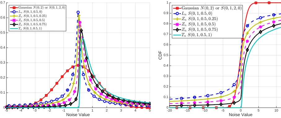
are depicted in Figs. 2 and 3, respectively.

Remark 1: In [52] it is shown that for an infinite, three-dimensional homogeneous medium without flow, and a spher-ically absorbing receiver, the first arrival time follows a scaled L´evy distribution. Therefore, the results presented in this paper can be extended to 3-D space by simply introducing a scalar multiple in the noise distribution.

B. System B

To find the noise distribution of the system in (2), we first discuss the class of probability distributions known as stable distributions[28], [53]. Note that the L´evy distribution belongs to this class.

Definition 2 (Stable Distributions): A RV X has a stable distribution if for two independent copies X1 and X2, and

positive constantsa1, a2, a3∈ R+ anda4∈ R, the following

holds:

a1X1+a2X2 d

=a3X+a4.

Stable distributions can also be defined via their character-istic function.

Definition 3 (Characteristic Function of a Stable Distribu-tion):Let−∞< µ <∞, c≥0,0< α≤2, and−1≤β ≤1. Further define:

Φ(ω, α)_,

(

tan πα₂

, α6= 1

−2

πlog(|ω|), α= 1 .

Then, the characteristic function of a stable RV X, with lo-cation parameterµ, scale parameterc, characteristic exponent

α, and skewness parameterβ, is given by:

ϕ(ω;µ, c, α, β) = exp [jµω− |cω|α_{(1−jβsgn(ω)Φ(ω, α))].}

(7)

In the following, we use the notation S(µ, c, α, β) to represent a stable distribution with the parametersµ, c, α, and

Noise Value

-5 -4 -3 -2 -1 0 1 2 3 4 5

PDF

0 0.1 0.2 0.3 0.4 0.5 0.6 0.7

GaussianN(0;2) orS(0;1;2;0) LnS(0;1;0:5;0)

[image:5.612.285.559.52.245.2]

ZnS(0;1;0:5;0:25) ZnS(0;1;0:5;0:5) ZnS(0;1;0:5;0:75) TnS(0;1;0:5;1)

Fig. 2. The probability density function of different standardized noise terms.

β does not matter in this case and can be assumed to be zero), the L´evy distribution with α=1₂ andβ= 1, and the Cauchy distribution with α= 1andβ = 0. Generally, the parameters

α and β define a subclass within the stable distribution family. Next, we introduce some important properties of stable distributions [28].

Property 1: LetX ∼S(µ, c, α, β), and defineY = X−_cµ. Thenf(x)dx=f(y)dy, andY is called the standard form of

X.

Property 2:LetX˜ ∼_S(0,1, α, β)be the standard form of a stable RV with parameters αandβ. Then the PDF and the CDF of any RV X∼S(µ, c, α, β)can be calculated as

fX(x) = fX˜

x−µ c

c , (8)

FX(x) =FX˜( x−µ

c ). (9)

Using this property, the standard PDF and CDF of a stable RV can be used to calculate probabilities involving non-standard stable RVs just like the way the standard Gaussian PDF and CDF are used to calculate probabilities involving non-standard Gaussian RVs.

Property 3: The PDFs of stable RVs with β = 0 are symmetric aroundµ.

Property 4: If X is a standardized (i.e., with µ = 0 and

c = 1) stable RV with parameters0< α < 2 andβ, then as

x→ ∞,

P(X > x;α, β)≈ 1 +β

πxα Γ(α) sin

_απ

2

. (10)

Remark 2: Using this property it can be shown that for a stable distributed RV X with parameter α, the moments of order greater thanα(i.e.,E[|X|α]) are infinite. Therefore, all

stable distributions withα <2have infinite variances, and all stable distributions with α <1have infinite mean values.

With these definitions we now model the noise term Ln in

(2).

Theorem 1: LetcB= 2d

2

D, where dis the distance between

the transmitter and the receiver and D is the diffusion

co-Noise Value

-20 -15 -10 -5 0 5 10 15 20

CDF

0 0.1 0.2 0.3 0.4 0.5 0.6 0.7 0.8 0.9 1

GaussianN(0;2) orS(0;1;2;0)

LnS(0;1;0:5;0) ZnS(0;1;0:5;0:25) ZnS(0;1;0:5;0:5) ZnS(0;1;0:5;0:75) TnS(0;1;0:5;1)

Fig. 3. The cumulative distribution function of different standardized noise terms.

efficient of the information particles. Then, the characteristic function of the noise term Ln is given by:

ϕ(ω;cB) = exp

h

−pcB|ω|

i

,

which implies that Ln∼S(0, cB,1₂,0).

Proof:We know thatLn=Tn2+(−Tn1)withTn2, Tn1 ∼

S(0, cA,1₂,1), where cA = d

2

2D. Since Tn1 and Tn2 are

independent, the characteristic function forLn is given by

ϕLn(ω) =ϕTn2(ω)ϕTn1(−ω) (11)

= exph−p|cAω|(1−jsgn(ω))

i

×

exph−p

|cAω|(1 +jsgn(ω))

i

(12)

= exph−p|4cAω|

i

. (13)

Thus, using the expression in (7) we conclude that Ln ∼

S(0, cB,1₂,0).

Remark 3:If the same type of particle is used in system A and system B, and the distance between the transmitter and the receiver is the same, then the scale parameter c in the noise term for system B is four times greater than the scale parameter for system A, i.e.,cB= 4cA.

To find an expression for the PDF of the noise termLn in

(2), we first define the following functions. Let K(a, b) and

L(a, b), a∈ R, b∈ R+_{, be the complex and imaginary Voigt}

functions [54], given by :

K(a, b)_, √1 π

Z ∞

0

exp(−t2_{/4) exp(−bt) cos(at)dt, (14)}

and

L(a, b)_, √1 π

Z ∞

0

exp(−t2_{/4) exp(−bt) sin(at)dt. (15)}

[image:5.612.57.510.55.246.2]

cases (e.g., b 0), analytical approximations of these func-tions exist in terms of elementary funcfunc-tions [40]. We further define:

G(u)_,p 1 8π|u|3

K

−_√1 8|u|,

1 √

8|u|

+L

−_√1 8|u|,

1 √

8|u|

. (16)

The PDF ofLn is stated in the following theorem:

Theorem 2: LetLn∼S(0, cB,12,0). Then the PDF of Ln

is given by:

fLn(`n) =

(₁

cBG

`n

cB

, `n6= 0

2

cBπ, `n= 0

. (17)

Proof: The proof is provided in Appendix A.

In this work, we do not provide an expression for the CDF of the noise terms FLn(`n), and it would be difficult

to integrate (2) to obtain the CDF. However, the CDF can be calculated numerically using the methods described in [55, Sec. 3]. Moreover, tables of the standardized CDF could be used to calculate probabilities involving the noise term. Figs. 2 and 3 depict the PDF and CDF for the standardized noise term Ln withcB= 1.

C. System C

We first note that the noiseZngiven in (3) is fundamentally

different from the noise Ln in system B since the two

different types of information particles may have different diffusion coefficients. Let Da be the diffusion coefficient of

information particlea, andDb be the diffusion coefficient for

the information particle b. We define cC ,

d2₍√_D

a+ √

Db)2

2DaDb , βC ,

√

Da− √

Db √

Da+ √

Db. Furthemore, without loss of generality, we

assume that particle a is released before particle b. We now model the noise term Zn in (3).

Theorem 3: The characteristic function for the noise term

Zn is given by:

ϕ(ω;cC, βC) = exp

h

−p

cC|ω|(1−jβCsgn(ω))

i ,

which implies thatZn∼S 0, cC,12, βC

.

Proof: First, note that Zn = Tnb + (−Tna) with Tna, Tnb ∼ S(0, ci,

1

2,1), where ci = d2

2Di for i ∈ {a, b}.

SinceTnaandTnb are independent, the characteristic function

of Zn is given by:

ϕZn(ω)

=ϕT_nb(ω)ϕT_na(−ω) (18)

= exph−√cb

p

|ω|(1−jsgn(ω))i×

exph−√ca

p

|ω|(1 +jsgn(ω))i (19)

= exph−p|ω|(√cb+ √

ca−jsgn(ω)( √

ca− √

cb))

i (20)

= exph−(√cb+ √

ca)

p

|ω|×

1−jsgn(ω) √

ca− √

cb √

cb+ √ ca (21) = exp

−d( √

Da+ √

Db) √

2DaDb

p

|ω|×

1−j √

Da− √

Db √

Da+ √

Db

sgn(ω)

. (22)

Thus, using the expression in (7) we conclude that Zn ∼

S 0, cC,1₂, βC

.

Remark 4: When the diffusion coefficients of the two particles are approximately the same, i.e., Da ≈ Db, the

distribution ofZnapproaches the distributionLn(i.e.βC≈0).

On the other hand, when Da Db or Da Db, then βC≈ ±1which implies thatZnis L´evy distributed. Therefore,

when one information particle has a much higher diffusion coefficient than the other, system C can be reduced to system A with the added benefit that no synchronization is required between the transmitter and the receiver. However, this comes at a cost of: 1) Using two particles instead of one; and 2) The resulting system A has a scaling parameter that corresponds to the smaller diffusion coefficient.

To derive the PDF ofZn we first define the following two

functions:

G+(u, β),

1

p

8π|u|3

(1 +β)K

−√1+β 8|u|,

1−β √

8|u|

+(1−β)L

−√1+β 8|u|,

1−β √

8|u|

, (23)

G−(u, β), 1

p

8π|u|3

(1−β)K

1−β √

8|u|,

1+β √

8|u|

+(1 +β)L

1−β √

8|u|,

1+β √

8|u|

, (24)

where K(a, b) and L(a, b) are the real and imaginary Voigt functions given in (14) and (15), respectively. The PDF ofZn

is now stated in the following theorem:

Theorem 4: Let Zn ∼ S(0, cC,1₂, βC). Then the PDF of Zn is given by:

fZn(zn) =

       1 cCG+

zn

cC, βC

, zn >0

2(1−β2₎

cCπ(1+β2)2, zn = 0

1 cCG−

zn

cC, βC

, zn <0

. (25)

Proof:The proof is provided in Appendix B.

Again, we do not provide an expression for the CDF of the noise terms FZn(zn), instead we note that it can be

2 and 3 depict the PDF and CDF for the standardized noise term Zn withcC = 1 and four different values for βC. Note

that forβC= 0the distribution and the density functions of the

noiseZn in System C are the same as the noiseLn in system

B. This is due to the diffusion coefficient of type-aand

type-b particles being equal, which means that both particle types have the same random propagation delay characteristics.

Remark 5:Moving from a 1-D space to a 3-D space, there is a probability that the particle will never arrive at the receiver (see [52]). For systems B and C, both particles must arrive for error free communication. Conditioned on the event that the two particles arrive, the noise distribution will be the same as the 1-D case. Therefore, in 3-D, the noise distribution will be scaled by the probability of the event that both particles arrive.

IV. OPTIMALDETECTION INBINARYDBMT SYSTEMS

In this section, we consider equiprobable binary transmis-sion over the three different DBMT systems. Using the noise models developed in the previous section, we characterize the optimal detection rule for each modulation.

A. System A

For system A, we assume that the transmission symbols are

Tx ∈ {0,∆}, where ∆ >0. Using Property 2, we write the

distribution of the output probability, conditioned on the input, in terms of the standard L´evy distribution T˜n ∼L(0,1) as

follows:

fTy|Tx(ty|Tx= 0) =fTn(ty) =

fT˜n(ty/cA) cA

, (26)

fTy|Tx(ty|Tx= ∆) =fTn(ty−∆) = f_T˜

n (ty−∆)/cA

cA

.

(27)

As the two transmitted symbols are equiprobable, the de-tector that minimizes the probability of error is the maximum likelihood (ML) detector. In this work we assume both the 0-bit and the 1-0-bit are equiprobable and apply the ML detector. In this case, the likelihood ratio is given by:

ΛA(ty) =

fTy|Tx(ty|Tx= 0)

fTy|Tx(ty|Tx= ∆)

, (28)

and optimal detection can be done by a comparison of the log likelihood ratio (LLR) to zero, i.e.,

log(ΛA(ty)) Tx= 0

≷

Tx= ∆

0. (29)

Note that the proof of the existence of the optimal threshold value is straightforward using the fact that stable distributions are unimodal [53, Theorem 2.7.6], and that for the noise term

Tn the mode is at c/3. Therefore, there exists a threshold

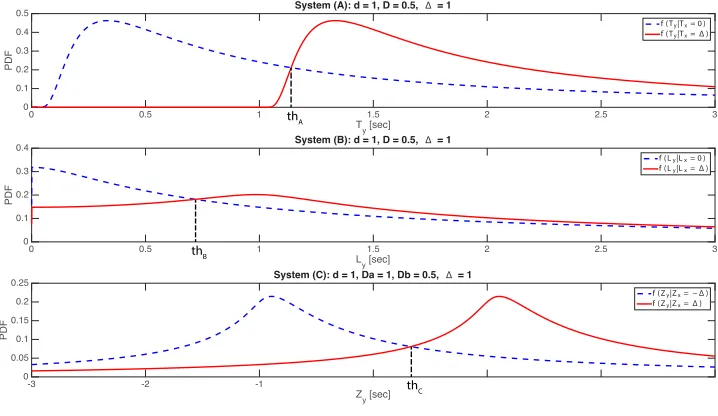
∆ <thA≤c/3 + ∆, such that ΛA(t)>1 for t < thA and ΛA(t)≤ 1 for t ≥thA [26], [27]. The top plot in Figure 4

shows the optimal threshold for the case when ∆ = 1, the distance is d= 1and the diffusion coefficient isD= 0.5.

The probability of error for system A is now given by:

P_eA=P(Tx= 0)Pr(ty>thA|Tx= 0)

+P(Tx= ∆)Pr(ty≤thA|Tx= ∆), (30)

= 0.5Pr(tn>thA) + 0.5Pr(tn≤thA−∆) (31)

= 0.5[1−F_T˜_n(th_cA

A) +FT˜n( thA−∆

cA )], (32)

whereF_T˜

n(t)is the CDF of a standard L´evy RV.

B. System B

For system B we assume that the input is Lx ∈ {0,∆},

where Lx = 0 represents two particles released

simultane-ously, while Lx = ∆ represents two particles released ∆

seconds apart. Let L˜n ∼ S(0,1,1₂,0) be the standard form

of the noise term in (2). The PDF of the outputLy, given the

inputLx, is provided in the following proposition:

Proposition 1:The system outputLy, given the system input Lx, has the PDF:

fLy|Lx(`y|Lx= 0) =

      

2fLn˜ `y

cB

cB `y>0

2

(cBπ) `y= 0

0 `y<0

, (33)

fLy|Lx(`y|Lx= ∆) =

        

f˜_Ln `y_c−∆ B

+f˜_Ln −`y_c−∆ B

cB `y>0

f˜_{Ln c}∆ B

cB `y= 0

0 `y<0

.

(34)

Proof: It is clear from the system definition that when

Ly <0 the PDF is 0 (i.e. the time between two arrival times

is not negative). WhenLy= 0, we havefLy|Lx(0|Lx= 0) = fLn(0), andfLy|Lx(0|Lx= ∆) =fLn(∆). To derive the PDF

value for Ly >0, we use the fact that the CDF ofLy given Lx=x≥0 can be obtained from the CDF ofL˜n as

FLy|Lx(`y|Lx=x) = Pr(Ly≤`y|Lx=x)

= Pr(|x+Ln| ≤`y)

= Pr(−`y≤x+Ln≤`y)

= Pr(−`_cy−x

B ≤

˜ Ln ≤

`y−x

cB )

=FL˜n

`y−x

cB

−FL˜n −`y−x

cB

.

By differentiating with respect to `y, and setting x= 0 and x= ∆, we obtain (33) and (34), respectively.

Similarly to (28), the likelihood ratio for the ML detector for system B is given by:

ΛB(`y) =

fLy|Lx(`y|Lx= 0)

fLy|Lx(`y|Lx= ∆)

. (35)

The following theorem states that, just like in the case of system A, the ML detector can be implemented by comparing

log(ΛB(`y))to zero:

Theorem 5: There exists a fixed threshold thB > ∆₂ such

that the ML detector in the case of system B is given by:

log(ΛB(`y)) Tx= 0

≷

Tx= ∆

Ty [sec]

3 5

. 2 2

5 . 1 1

5 . 0 0

PDF

0 0.1 0.2 0.3 0.4

0.5 System (A): d = 1, D = 0.5, ∆ = 1

f(Ty|Tx= 0 ) f(Ty|Tx=∆)

L_y [sec]1.5 2 2.5 3

1 5

. 0 0

PDF

0 0.1 0.2 0.3

0.4 System (B): d = 1, D = 0.5, ∆ = 1

f(Ly|Lx= 0 ) f(Ly|Lx=∆)

Zy [sec]

1 -2

-3

-PDF

0 0.05 0.1 0.15 0.2

0.25 System (C): d = 1, Da = 1, Db = 0.5, ∆ = 1

f(Zy|Zx=−∆) f(Zy|Zx=∆)

thA

thB

[image:8.612.127.486.57.265.2]

thC

Fig. 4. The ML optimal decision threshold for the three systems.

Proof: The proof is provided in Appendix C.

The middle plot in Fig. 4 depicts the optimal threshold for the case when ∆ = 1, the distance is d = 1 and the diffusion coefficient is D = 0.5. Since the closed-form expression for the CDF of the noise term is unknown, this threshold is calculated numerically. Finally, the probability of error for binary communication over system B is given by:

P_eB=P(Lx= 0)Pr(Ly>thB|Lx= 0)

+P(Lx= ∆)Pr(Ly ≤thB|Lx= ∆),

= 0.5(Pr(Ln>thB) + Pr(Ln≤ −thB)) + 0.5Pr(−thB−∆≤Ln≤thB−∆),

= 0.5(Pr( ˜Ln> th_cB

B) + Pr( ˜Ln≤ −

thB cB))

+ 0.5Pr(−thB−∆

cB ≤

˜

Ln≤thB_c−∆

B ),

=F_L˜_n th_cB B

+ 0.5 F_L˜_n thB_c−∆ B

−F_L˜_n thB_c+∆ B

. (37)

Thus, similarly to the case of system A, the probability of error can be calculated using the standard form of the noise term.

C. System C

Recall that for system C the two particles are distinguish-able, and Zx = Txb−Txa is the time interval between the

releases of particlesb anda. Here, we assume information is encoded in the orderof release. The inputZx∈ {−∆,∆} is

now given by:

Zx=

(

∆, Txa= 0, Txb= ∆ −∆, Txb= 0, Txa= ∆

. (38)

Note that similarly to systems A and B, the information is encoded over the time period ∆.

Let Z˜n ∼ (0,1,1₂, βC) be the standard form of the noise

term in (3). Then the PDF of the output given the input is

given by

fZy|Zx(zy|Zx=−∆) =

f_Z˜_n zy_c+∆ C

cC

(39)

fZy|Zx(zy|Zx= ∆) = f_Z˜

n

zy−∆

cC

cC

. (40)

Again, to minimize the probability of error at the receiver, the ML detector is used. Let thC be the optimal ML detection

threshold for this system. It is easy to see that this threshold exists for system C since stable distributions are unimodal and the two PDFs are shifted versions of each other. The bottom plot in Figure 4 shows the optimal threshold for the case when

∆ = 1, the distance isd= 1and the diffusion coefficients are

Da = 1 andDb= 0.5. The probability of error is now given

by:

P_eC=P(Zx=−∆)Pr(zy >thC|Zx=−∆)

+P(Zx= ∆)Pr(zy≤thC|Zx= ∆),

= 0.5Pr(zn>thC+ ∆) + 0.5Pr(zn≤thC−∆) = 0.5[1−F_Z˜

n(thC+ ∆) +FZ˜n(thC−∆)], (41)

which can be calculated using the CDF of the standard form of the noise term.

V. GEOMETRICPOWER ANDG-SNR

statistics, i.e., it is based on logarithmic “moments” of the form _E[log|N|].

Definition 4 (Geometric Power): The geometric power of the RV N is given by:

S0(N),eE[log|N|]. (42)

In the following we use the terms noise power and the geometric power of the noise interchangeably.2

In [41, Prop. 1], an expression for the geometric power of a symmetric stable distribution is presented. Property 3 implies that symmetric stable distributions are in fact S(0, c, α,0). This expression can therefore be used to calculate the geo-metric power of the noise term LN in system B. Yet, this

expression is not applicable for the noise terms of systems A and C in which β 6= 0. The following theorem characterizes the geometric power of almost all stable distributions:

Theorem 6:LetN ∼S(0, c, α, β), whereα6= 1, orα= 1

andβ = 0. Then, the geometric power ofN is given by:

S0(N) =cG(1/αγ −1) 1 +β

2_tan2₍πα 2 )

1/(2α)

, (43)

whereGγ =eγ, andγ≈0.5772 is the Euler’s constant [56,

Ch. 5.2].

Proof: The proof is provided in Appendix D.

Remark 6: For the systems considered in this paper, since

α= 1₂, the noise power simplifies to:

S0(N) =cGγ 1 +β2

. (44)

Note that in this case, the noise power increases with respect toβ (the degree of skewness) andc(the scale parameter).

We now define the geometric SNR (G-SNR) as in [41, Section III]:

Definition 5 (Geometric Signal-to-Noise Ratio): Let X be the input signal in an additive-noise channel with a random noiseN. Then the G-SNR is defined as:

G-SNR_, 1 2Gγ

_X

max−Xmin S0(N)

2

, (45)

where Xmax and Xmin are the maximum and minimum

admissible values for the channel input X. The normalizing term _2G1

γ is used to ensure that the G-SNR corresponds to

the standard SNR in the case of an additive Gaussian noise channel.

Using this definition and Theorem 6, the G-SNR for systems A and C is defined as follows:

G-SNRA=

1 2Gγ

∆ 2cAGγ

2

, (46)

G-SNRC =

1 2Gγ

_2∆

cCGγ(1 +βC2)

2

. (47)

Remark 7: Note that system B involves an absolute value operation, thus, the G-SNR of system B cannot be obtained based on the techniques used to derive the G-SNR for systems A and C. Since the absolute value operation can only degrade the detection performance, calculating the G-SNR of the

2_{Note that the definition of geometric power/SNR we introduce here is}

different from the one widely used in RF communications.

" [sec]

0 5 10 15 20

Probability of Bit Error

0.14 0.15 0.16 0.17 0.18 0.19 0.2 0.21 0.22 0.23

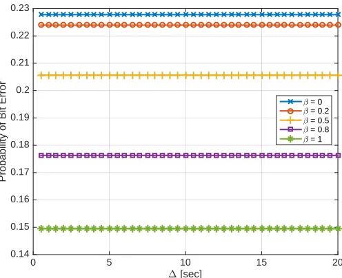
[image:9.612.314.562.54.256.2]

- = 0 - = 0.2 - = 0.5 - = 0.8 - = 1

Fig. 5. This plot shows that for a constant G-SNR, the BER is constant. For each point, the parametercof the noise distribution is calculated using the corresponding value for∆such that the G-SNR= 1.

system Ly =Lx+Ln can serve as an upper bound on the

G-SNR of system B. This upper bound is given by:

G-SNRB ≤G-SNRubB =

1 2Gγ

_∆

cBGγ

2

. (48)

This implies that the BER of the ML detector for system B is higher than the BER of the ML detector for the system

Ly=Lx+Ln, as indicated in Section VI.

Remark 8: When the diffusion coefficient and the distance between the transmitter and the receiver are the same, the G-SNR of system A is four times larger than the G-G-SNR of system B sincecB= 4cA. This implies that on top of the fact

that two information particles are released in system B while only a single particle is released in system A, the gain from synchronization is a factor of 1₄ in the noise geometric power.

Remark 9:For system C let r=Da/Db be the ratio of the

diffusion coefficient of the two information particles. Then the noise parameters can be written as cC =

d2₍√_r+1)2 2rDb and βC =

√

r−1

√

r+1. Next, assume that the diffusion coefficient Db

is fixed, and the diffusion coefficient of Da can be changed.

In this case the noise geometric power is proportional to 1_r, which decreases asr increases. This also implies that the G-SNR increases with r. From the expression for βC and cC

we observe that βc → 1 and cC → d

2

2Db, when r → ∞.

Thus, in this case, system C reduces to system A, while no synchronization is required between the transmitter and the receiver. Yet, this comes at a cost of using two different information particles. Note that this cost is captured in the G-SNR expression since the geometric power of the transmitted signal in system C is four times that of systems A and B, which can result in as much as 4 times improvement in G-SNR.

VI. NUMERICALEVALUATION

" [sec]

0 5 10 15 20

Probability of Bit Error

0.08 0.09 0.1 0.11 0.12 0.13 0.14 0.15

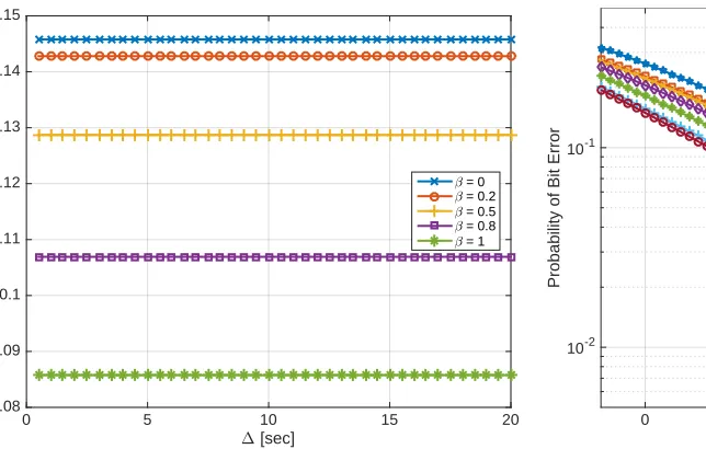
[image:10.612.63.385.53.258.2]

- = 0 - = 0.2 - = 0.5 - = 0.8 - = 1

Fig. 6. This plot shows that for a constant G-SNR, the BER is constant. For each point, the parametercof the noise distribution is calculated using the corresponding value for∆such that the G-SNR= 10.

modulation schemes. In the additive white Gaussian noise channel the BER of the ML detector is only a function of SNR, namely, for a fixed SNR, the individual values of the signal power and the noise power do not affect the BER. To evaluate if this property also holds for the three MT systems, we consider system C which can be specialized to both systems A and B using different values of the parameterβC, see (46)–

(47). Thus, we evaluate if a constant BER is observed for a fixed value of G-SNR.

Figs. 5 and 6 depict BER versus ∆ for two values of G-SNR: 1 and 10. In these plots, the x-axis corresponds to the values of∆. For each point in the plot, the value of the noise parametercCis calculated such that G-SNR is either 1 (Fig. 5)

or 10 (Fig. 6). The BER is then numerically calculated using these values based on (41). It can clearly be observed that the BER is constant for a given G-SNRregardlessof the value of

∆ andcC. It can further be observed that the BER decreases

as βC→1, which is in agreement with Remark 9.

Fig. 7 depicts the BER versus G-SNR for the different modulation techniques. For system C, five different values of

βC= 0,0.25,0.5,0.75,0.95are considered. The asynchronous

scheme in system B with indistinguishable particles achieves the highest BER, while system A, which assumes perfect syn-chronization, achieves the lowest BER. The gap between these can be thought of as the cost of having no synchronization. Note that in system A, a single particle is released, while in system B two particles are released.

For system C it can be observed that by using two distin-guishable particles, the BER improves compared to system B. Note that when βC = 0 the noise distribution is the

same as that in system B. In this case, when the dispersion parameter c is the same for both systems, the G-SNR of system C is four times larger than G-SNRubB in (48). Yet,

Fig. 7 indicates that even for βC = 0 the BER of system

C is lower than the BER of system B. This demonstrates the

G-SNR [dB]

0 10 20 30 40 50

Probability of Bit Error

10-2 10-1

System B System C

-c=0 System C

-c=0.25 System C

-c=0.50 System C

-c=0.75 System C

[image:10.612.304.560.53.257.2]

-c=0.95 System A

Fig. 7. BER versus G-SNR in dB for each modulation scheme.

destructive effect of the absolute value operation as indicated in Remark 7. Finally, we observe that as βC increases the

BER of system C decreases, while when βC → 1 the BER

of system C approaches the BER of system A. In this case, asynchronous communication is possible with the same BER performance as synchronized communication at the cost of using two distinguishable particles.

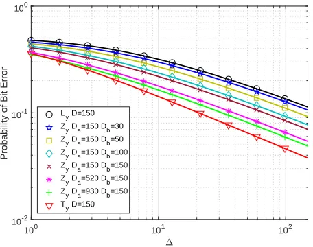
We conclude the numerical evaluations with a case study. We consider a DBMT system where the distance between the transmitter and the receiver is d= 20 µm. Assume that the receiver is capable of detecting insulin molecules, which has a diffusion coefficient of DI = 150 µm2/s [3]. From these

values the noise parameters cA andcB can be calculated for

the modulation techniques represented by systems A and B. For system C, we consider six different particles as candi-dates for the second distinguishable particle. These particles are assumed to have diffusion coefficients ranging from 30

µm2/s (e.g., diffusion coefficient of DNA) to 930µm2/s (e.g., diffusion coefficient of glycerol).

Fig. 8 depicts the results. In order to further evaluate the correctness of the analytical results, we also perform Monte Carlo simulations. It can be observed that the theoretical re-sults (line plots) match perfectly with the rere-sults of the Monte Carlo simulations (point plots). The asynchronous modulation scheme in system B with indistinguishable particles has the highest BER. Note that even the modulation scheme in system C where the diffusion coefficient of the second particle is one fifth of the diffusion coefficient of the particles used in system B (i.e. 30µm2/s) has lower BER. For the modulation technique in system C, as the diffusion coefficient of the second particle increases, the BER decreases. The modulation in system A achieves the best BER performance, and this shows that transmitter-receiver synchronization could have a considerable effect on BER. Table I quantifies the BER for each case.

100 101 102 10-2

10-1 100

Probability of Bit Error

L_y D=150

Z_y D_a=150 D_b=30

Z_y D_a=150 D_b=50

Z

y Da=150 Db=100 Z_y D_a=150 D_b=150

Z_y D_a=520 D_b=150

Z_y D_a=930 D_b=150

T y D=150

Fig. 8. BER versus∆under different modulation schemes. The line plots are based on the theoretical results derived in the paper, and the point plots are the corresponding Monte Carlo simulation results.

TABLE I

THEBEROF DIFFERENT MODULATIONS IN THE CASE STUDY FOR

DIFFERENT VALUES OF∆. FOR THE MODULATION SCHEME IN SYSTEMC

THE TERM IN PARENTHESIS IS THE DIFFUSION COEFFICIENT OF THE

SECOND PARTICLE.

∆ 1 25 50 75 100

System A 0.3590 0.0912 0.0648 0.0530 0.0460 System B 0.4778 0.2346 0.1799 0.1523 0.1348 System C (D= 30) 0.4592 0.2202 0.1687 0.1428 0.1263 System C (D= 150) 0.4073 0.1535 0.1145 0.0957 0.0841 System C (D= 930) 0.3533 0.1109 0.0812 0.0674 0.0589

This can be achieved by properly spacing the transmissions leading to relatively large symbol durations. We now discuss how large this duration should be for the different considered systems. Let Tsymbol denote the spacing between consecutive

transmissions, and0< pclean<1. Further, letTlastdenote the

last particle arrival timecalculated over the particles released in the current channel use. We propose to chooseTsymbolsuch

that:

Pr{Tlast≤Tsymbol}=pclean.

Hence, if pclean is a (fixed) value close to 1, then with high

probability all the released particles arrive at the receiver before Tsymbol, implying that after this idle duration the

channel can be used for another transmission. Moreover, the symbol durationTsymbolcan be found from the CDF of Tlast

as a function of pclean. Note that the CDF ofTlastis different

for each system considered. Yet, AssumptionA3) implies that for all three systems the CDF of Tlast is the product of the

CDFs of the propagation time of the individual particles (in the case of System A it is simply the CDF of the L´evy distribution).

Fig. 9 depicts the calculated Tsymbol for the different

systems with different diffusion coefficients. pclean was set

to 0.99. It can be observed that due to the heavy tails of the propagation density, the symbol duration is almost constant

100 101 102 103

Δ

0 1 2 3 4 5 6 7 8 9

Symbol Duration

×104

Sys. B D=150 Sys. C D_a=150 D_b=30

Sys. C Da=150 Db=50

Sys. C Da=150 Db=100

Sys. C D_a=150 D_b=150

Sys. C D_a=520 D_b=150

Sys. C D_a=930 D_b=150

[image:11.612.63.291.57.237.2]

Sys. A D=150

Fig. 9. Tsymbolversus∆under different modulation schemes, forpclean=

0.99.

as a function of ∆, and is much larger than ∆. It can further be observed that the order of the curves in Fig. 9 is almost identical to the order of the curves in Fig. 8, where the exception is the curve corresponding to System B which requires almost the sameTsymbol as System C with the same

[image:11.612.330.537.63.236.2]

diffusion coefficients. Note that the modulation in system A requires the smallestTsymbol, thus, together with the results of

Fig. 8, we conclude that the performance gains obtained from transmitter-receiver synchronization are significant.

VII. CONCLUSIONS ANDFUTUREWORK

[image:11.612.51.302.358.419.2]

As part of future work, we will explore extending the results to the case where multiple information particles are released simultaneously instead of one. Note that some of our current ongoing work has shown that simultaneously releasing multiple particles can improve the performance of the first system significantly [24], [27]. We would like to extend these results to the asynchronous systems presented in this paper using order statistics.

APPENDIXA

PROOF OFTHEOREM2

We use Property 2, and find an expression for the standard-ized distribution with cB= 1. Then the PDF for any value of cB can be calculated using (8). Let X ∼S(0,1,1₂,0) be a

standardized stable RV with parameters α= 1₂ and β = 0. Then the PDF ofX is given by [57, Eq. (7.1)]:

f(x; 1/2, β) =<n z πx[

√

πe−z2−2jD(z)]o, (49)

where

D(z) =e−z2

Z z

0

et2dt (50)

is the Dawson’s Integral [56, Eq. (7.2.5)], and

z= 1 +β−j(1−β)

2√2x . (51)

It is possible to rewrite (49) in terms of the complex error function, also known as Faddeeva function or the Kramp function [56, Eq. (7.2.3)]:

w(z) =e−z2

1 + √2j π

Z z

0 et2dt

=e−z2erfc(−jz). (52)

Using [56, Eq. (7.5.1)]:

D(z) = 0.5j√π(e−z2−w(z)), (53)

and the propertyw(−z) = 2e−z2−w(z), we rewrite (49) as:

f(x; 1/2, β) =<

z √

πxw(−z)

. (54)

One of the benefits of writing the PDF in terms of the complex error function is that there are a large body of works that considered calculating it numerically. Moreover, ifz=a+jb, for b > 0 the complex error function can be represented by its real and imaginary parts as [37, Sec. 1]:

w(a+jb) =K(a, b) +jL(a, b), b >0, (55)

where K(a, b) and L(a, b) are the real and imaginary Voigt functions given in (14) and (15), respectively.

Using Property 3, the PDF of X is symmetric. Hence, the density for X ≥0 is sufficient for characterizing the whole PDF. Sinceβ = 0, when X >0, we can writez=px−jpx

where px = 1/ √

8x. Substituting (55) in (54), the density of

X, when X≥0, can be written as:

f(x) =

( ₁

√

8πx3[K(−px, px) +L(−px, px)] x >0 2

π x= 0

, (56)

where the value for x = 0 follows from [53, Eq. (2.2.11)]. Finally, the density for X < 0 is obtained using symmetry. The proof is completed by applying (8).

APPENDIXB PROOF OFTHEOREM4

We use Property 2, and find an expression for the standard-ized distribution withcC= 1. Thus, the PDF for any value of cC can be calculated using (8). LetX ∼S(0,1,1₂, βC)be the

standardized stable RV with parametersα=1

2 andβC. Using

(54), and recalling thatβC= ( √

Da− √

Db)/( √

Da+ √

Db),

we write (51) as z = px − jqx when x > 0, where px= (1+βC)/(

p

8|x|)andqx= (1−βC)/(

p

8|x|). Similarly, we write (51) asz=−qx−jpx whenx <0. Using (54) and

the Voigt functions decomposition of the Faddeeva function (55), the PDF of the standardized distribution is given by:

f(x;βC) =

                          

1

√

8πx3

(1 +βC)K(−px, qx)

+ (1−βC)L(−px, qx)

, x >0

2(1−β2)

π(1+β2₎2, x= 0

1 √

8π|x|3

(1−βC)K(qx, px)

−(1 +βC)L(qx, px)

, x <0 ,

where, again, the value for x = 0 follows from [53, Eq. (2.2.11)]. The proof is completed by applying (8).

APPENDIXC PROOF OFTHEOREM5

We first observe that for `y = 0, fLy|Lx(0|0) > fLy|Lx(0|∆). This follows from the fact that stable

distribu-tions are unimodal, and the mode of the noise term Ln is

at ` = 0. Therefore, the threshold is located at thB > 0,

and we focus of the case where `y > 0. Note that in

this case, due to the continuity and unimodality of stable distributions [53, Theorem 2.7.6], bothfLy|Lx(`y|Lx= 0)and fLy|Lx(`y|Lx = ∆) are continuous functions and unimodal.

We now have the following lemma:

Lemma 1: If 0 < `y ≤ ∆<sub>2</sub>, then fLy|Lx(`y|Lx = 0) > fLy|Lx(`y|Lx= ∆).

Proof: We first consider the system in (2) without the absolute value: L˜y = Lx + Ln. Here, fL˜y|Lx(˜ly|lx) = fLn(˜ly−lx). Since stable distributions are unimodal, we have f_L˜

y|Lx(˜ly|Lx = 0) > fL˜y|Lx(˜ly|Lx = ∆),∀ ˜

ly < ∆₂. Using

the expression for the PDF of system (2) in (33)–(34) we obtain the desired result.

Lemma 2: If `y > ∆₂, then there exists a point thB

such that for all ∆₂ < `y < thB, fLy|Lx(`y|Lx = 0) > fLy|Lx(`y|Lx = ∆) and for all `y > thB, fLy|Lx(`y|Lx = 0)≤fLy|Lx(`y|Lx= ∆).

Proof: Note that for `y > ∆<sub>2</sub>, fLn(`y)< fLn(`y−∆).

Moreover, note that fLn(`) is a smooth function and it is

decreasing for ` > 0. Then clearly there exists a thB > ∆₂

such that: (

fLn(`y)−fLn(`y−∆)> fLn(`y+ ∆)−fLn(`y) `y<thB fLn(`y)−fLn(`y−∆)≤fLn(`y+ ∆)−fLn(`y) `y≥thB,

(57)

which follows since the slope offLn(`)for ` >0 decreases,

APPENDIXD PROOF OFTHEOREM6

To prove this theorem, we first derive E[|N|s]. We write

this expectation in integral form as:

E[|N|s] =

Z ∞

−∞

|n|s_{f(n; 0, c, α, β)dn}

(a)

=

Z ∞

0

nsf(n; 0, c, α, β)dn

+

Z ∞

0

nsf(n; 0, c, α,−β)dn,

where (a) follows since f(−x; 0, c, α, β) = f(x; 0, c, α,−β)

[28, Proposition 1.11]. Taking the derivative with respect tos

we obtain:

d dsE[|N|

s

] =

Z ∞

0

nslognf(n; 0, c, α, β)dn

+

Z ∞

0

nslognf(n; 0, c, α,−β)dn.

Further setting s= 0results in:

d dsE[|N|

s_]

_s=0

=E[log(|N|)].

We now define λ_,cαr_{1 +} β2 cot2₍πα

2 )

, and let

θ_,2 arctan

_β

cot(πα₂ )

/(πα).

Using [53, Fact 3, pg. 117], and [53, Theorem 2.6.4] we have that for N ∼S(0, c, α, β),α6= 1,

E[|N|s] =λs/α

cos(π₂θs)Γ(1−s/α)

cos(π₂s)Γ(1−s) . (58)

By taking the derivative of (58) with respect to sand evalu-ating the result at s= 0we obtain:

E[log(|N|)] = log(c) + 1 2αlog

1 + β

2

cot2(πα₂ )

+ (1/α−1)γ, (59)

whereγis the Euler’s constant [56, Ch. 5.2]. Finally, recalling that S0(N) =eE[log(|N|)] we conclude the proof.

ACKNOWLEDGMENT

The authors would like to thank Professor John P. Nolan at American University for providing valuable correspondence on stable distributions.

REFERENCES

[1] N. Farsad, W. Guo, C. B. Chae, and A. Eckford, “Stable distributions as noise models for molecular communication,” inProc. IEEE Global Communications Conference (GLOBECOM), Dec 2015, pp. 1–6. [2] N. Farsad, Y. Murin, W. Guo, C. B. Chae, A. Eckford, and A. Goldsmith,

“On the impact of time-synchronization in molecular timing channels,” in Proc. IEEE Global Communications Conference (GLOBECOM), 2016, pp. 1–6.

[3] N. Farsad, H. B. Yilmaz, A. Eckford, C.-B. Chae, and W. Guo, “A comprehensive survey of recent advancements in molecular communi-cation,”IEEE Communications Surveys & Tutorials, vol. 18, no. 3, pp. 1887–1919, 3Q 2016.

[4] T. Nakano, A. Eckford, and T. Haraguchi,Molecular communication. Cambridge University Press, 2013.

[5] W. Guo, T. Asyhari, N. Farsad, H. B. Yilmaz, A. Eckford, and C.-B. Chae, “Molecular communications: Channel model and physical layer techniques,”IEEE Wireless Communications, vol. 23, no. 4, pp. 120– 127, Aug. 2016.

[6] M. S. Kuran, H. B. Yilmaz, T. Tugcu, and I. F. Akyildiz, “Interference effects on modulation techniques in diffusion based nanonetworks,”

Nano Communication Networks, vol. 3, no. 1, pp. 65–73, Mar. 2012. [7] N.-R. Kim and C.-B. Chae, “Novel modulation techniques using

iso-mers as messenger molecules for nano communication networks via diffusion,”IEEE Journal on Selected Areas in Communications, vol. 31, no. 12, pp. 847–856, Dec. 2013.

[8] N. Farsad, A. Eckford, S. Hiyama, and Y. Moritani, “On-chip molecular communication: Analysis and design,”IEEE Transactions on NanoBio-science, vol. 11, no. 3, pp. 304–314, Feb. 2012.

[9] A. W. Eckford, “Timing information rates for active transport molecular communication,” in Nano-Net, ser. Lecture Notes of the Institute for Computer Sciences, Social Informatics and Telecommunications Engi-neering. Springer Berlin Heidelberg, 2009, vol. 20, pp. 24–28. [10] M. U. Mahfuz, D. Makrakis, and H. T. Mouftah, “On the characterization

of binary concentration-encoded molecular communication in nanonet-works,” Nano Communication Networks, vol. 1, no. 4, pp. 289–300, Dec. 2010.

[11] N. Farsad, A. W. Eckford, and S. Hiyama, “Channel design and optimization of active transport molecular communication,” inProc. of 6th International ICST Conference on Bio-Inspired Models of Network, Information, and Computing Systems, York, England, 2011.

[12] P. Lio and S. Balasubramaniam, “Opportunistic routing through conju-gation in bacteria communication nanonetwork,”Nano Communication Networks, vol. 3, no. 1, pp. 36–45, 2012. [Online]. Available: http://www.sciencedirect.com/science/article/pii/S1878778911000561 [13] A. Bicen and I. Akyildiz, “System-theoretic analysis and least-squares

design of microfluidic channels for flow-induced molecular communi-cation,”IEEE Transactions on Signal Processing, vol. 61, no. 20, pp. 5000–5013, Oct 2013.

[14] N. Farsad, W. Guo, and A. W. Eckford, “Tabletop molecular commu-nication: Text messages through chemical signals,”PLOS ONE, vol. 8, no. 12, p. e82935, Dec 2013.

[15] N. Farsad, W. Guo, and A. Eckford, “Molecular communication link,” inProc. IEEE Conference on Computer Communications (INFOCOM), 2014, pp. 107–108, live demo.

[16] B. H. Koo, C. Lee, H. B. Yilmaz, N. Farsad, A. Eckford, and C.-B. Chae, “Molecular MIMO: From theory to prototype,”IEEE Journal on Selected Areas in Communications, vol. 34, no. 3, pp. 600–614, March 2016.

[17] B. Atakan, S. Galmes, and O. Akan, “Nanoscale communication with molecular arrays in nanonetworks,” IEEE Transactions on NanoBio-science, vol. 11, no. 2, pp. 149–160, June 2012.

[18] B. Krishnaswamy, C. Austin, J. Bardill, D. Russakow, G. Holst, B. Hammer, C. Forest, and R. Sivakumar, “Time-elapse communication: Bacterial communication on a microfluidic chip,”IEEE Transactions on Communications, vol. 61, no. 12, pp. 5139–5151, Dec. 2013. [19] K. V. Srinivas, A. Eckford, and R. Adve, “Molecular communication

in fluid media: The additive inverse Gaussian noise channel,” IEEE Transactions on Information Theory, vol. 58, no. 7, pp. 4678–4692, July 2012.

[20] H. Li, S. Moser, and D. Guo, “Capacity of the memoryless additive inverse Gaussian noise channel,” IEEE Journal on Selected Areas in Communications, vol. 32, no. 12, pp. 2315–2329, Dec 2014.

[21] N. Farsad, Y. Murin, A. Eckford, and A. Goldsmith, “On the capac-ity of diffusion-based molecular timing channels,” IEEE International Symposium on Information Theory Proceedings (ISIT), 2016. [22] C. Rose and I. S. Mian, “Inscribed Matter Communication: Part I,”IEEE

Transactions on Molecular, Biological and Multi-Scale Communications, vol. 2, no. 2, pp. 209–227, Dec. 2016.

[23] ——, “Inscribed Matter Communication: Part II,”IEEE Transactions on Molecular, Biological and Multi-Scale Communications, vol. 2, no. 2, pp. 228–239, Dec. 2016.

[24] N. Farsad, Y. Murin, A. Eckford, and A. Goldsmith, “Capacity limits of diffusion-based molecular timing channels,” IEEE Transactions on Information Theory, submitted. [Online]. Available: http://arxiv.org/abs/1602.07757

[26] ——, “Communication over diffusion-based molecular timing channels,” in Proc. IEEE Global Communications Conference (GLOBECOM), 2016, pp. 1–6.

[27] ——, “Optimal detection for diffusion-based molecular timing chan-nels,” submitted toIEEE Journal on Molecular, Biological and Multi-scale Communication.

[28] J. P. Nolan, Stable Distributions - Models for Heavy Tailed Data. Boston: Birkhauser, 2015, in progress, Chapter 1 online at academic2.american.edu/∼jpnolan.

[29] A. P. Lee, “Microfluidic cellular and molecular detection for lab-on-a-chip applications,” in Proc. International Conference of the IEEE Engineering in Medicine and Biology Society, Sept 2009, pp. 4147– 4149.

[30] M. H. Horrocks, L. Tosatto, A. J. Dear, G. A. Garcia, M. Iljina, N. Cremades, M. Dalla Serra, T. P. J. Knowles, C. M. Dobson, and D. Klenerman, “Fast flow microfluidics and single-molecule fluores-cence for the rapid characterization of -synuclein oligomers,”Analytical Chemistry, vol. 87, no. 17, pp. 8818–8826, 2015.

[31] H. He, J. Lu, J. Chen, X. Qiu, and J. Benesty, “Robust blind identification of room acoustic channels in symmetric alpha-stable distributed noise environments,”The Journal of the Acoustical Society of America, vol. 136, no. 2, pp. 693–704, 2014. [Online]. Available: http://scitation.aip.org/content/asa/journal/jasa/136/2/10.1121/1.4884760 [32] S. Niranjayan and N. Beaulieu, “The BER optimal linear rake receiver for signal detection in symmetric alpha-stable noise,”IEEE Transactions on Communications, vol. 57, no. 12, pp. 3585–3588, Dec. 2009. [33] L. Fan, X. Li, X. Lei, W. Li, and F. Gao, “On distribution of SaS noise

and its application in performance analysis for linear rake receivers,”

IEEE Communications Letters, vol. 16, no. 2, pp. 186–189, Feb. 2012. [34] J. Wang, E. Kuruoglu, and T. Zhou, “Alpha-stable channel capacity,”

IEEE Communications Letters, vol. 15, no. 10, pp. 1107–1109, Oct. 2011.

[35] J. Fahs and I. Abou-Faycal, “On the capacity of additive white alpha-stable noise channels,” in Proc. IEEE International Symposium on Information Theory Proceedings (ISIT), July 2012, pp. 294–298. [36] F. Schrier, “The voigt and complex error function: A comparison

of computational methods,”Journal of Quantitative Spectroscopy and Radiative Transfer, vol. 48, no. 5/6, pp. 743–762, Nov.-Dec. 1992. [37] S. Abrarov and B. Quine, “Efficient algorithmic implementation of the

voigt/complex error function based on exponential series approxima-tion,”Applied Mathematics and Computation, vol. 218, no. 5, pp. 1894– 1902, 2011.

[38] M. R. Zaghloul and A. N. Ali, “Algorithm 916: Computing the faddeyeva and voigt functions,” ACM Trans. Math. Softw., vol. 38, no. 2, pp. 15:1–15:22, Jan. 2012. [Online]. Available: http://doi.acm.org/10.1145/2049673.2049679

[39] S. M. Abrarov and B. M. Quine, “A Rational Approxi-mation for Efficient Computation of the Voigt Function in Quantitative Spectroscopy,” Journal of Mathematics Research, vol. 7, no. 2, pp. 163–174, 2015. [Online]. Available: http://www.ccsenet.org/journal/index.php/jmr/article/view/46896 [40] “An assessment of some closed-form expressions for the voigt function,”

Journal of Quantitative Spectroscopy and Radiative Transfer, vol. 176, pp. 1–5, 2016.

[41] J. Gonzalez, J. Paredes, and G. Arce, “Zero-order statistics: A mathemat-ical framework for the processing and characterization of very impulsive signals,”IEEE Transactions on Signal Processing, vol. 54, no. 10, pp. 3839–3851, Oct. 2006.

[42] A. Noel, K. Cheung, and R. Schober, “Improving receiver performance of diffusive molecular communication with enzymes,”IEEE Transac-tions on NanoBioscience, vol. 13, no. 1, pp. 31–43, March 2014. [43] A. Einolghozati, M. Sardari, A. Beirami, and F. Fekri, “Capacity of

discrete molecular diffusion channels,” inProc. of IEEE International Symposium on Information Theory (ISIT), July 2011, pp. 723–727. [44] A. Einolghozati, M. Sardari, and F. Fekri, “Capacity of diffusion-based

molecular communication with ligand receptors,” in Proc. of IEEE Information Theory Workshop (ITW), Oct 2011, pp. 85–89.

[45] B. Atakan, “Optimal transmission probability in binary molecular com-munication,”IEEE Communications Letters, vol. 17, no. 6, pp. 1152– 1155, June 2013.

[46] T. Nakano, Y. Okaie, and J.-Q. Liu, “Channel model and capacity analysis of molecular communication with brownian motion,” IEEE Communications Letters, vol. 16, no. 6, pp. 797–800, June 2012. [47] H.-T. Chang and S. M. Moser, “Bounds on the capacity of the additive

inverse gaussian noise channel,” inIEEE International Symposium on Information Theory Proceedings (ISIT). IEEE, 2012, pp. 299–303.

[48] A. W. Eckford, K. Srinivas, and R. S. Adve, “The peak constrained additive inverse gaussian noise channel,” in IEEE International Sym-posium on Information Theory Proceedings (ISIT). IEEE, 2012, pp. 2973–2977.

[49] M. Pierobon and I. Akyildiz, “Capacity of a diffusion-based molecular communication system with channel memory and molecular noise,”

IEEE Transactions on Information Theory, vol. 59, no. 2, pp. 942–954, 2013.

[50] C. Rose and I. S. Mian, “Signaling with identical tokens: Upper bounds with energy constraints,” inIEEE International Symposium on Information Theory, 2014, pp. 1817–1821.

[51] I. Karatzas and S. E. Shreve,Brownian Motion and Stochastic Calculus. New York: Springer-Verlag, 1991.

[52] H. B. Yilmaz, A. C. Heren, T. Tugcu, and C.-B. Chae, “Three-dimensional channel characteristics for molecular communications with an absorbing receiver,”IEEE Communications Letters, vol. 18, no. 6, pp. 929–932, June 2014.

[53] V. Zolotarev,One-dimensional stable distributions. American Mathe-matical Soc., 1986, vol. 65.

[54] B. Armstrong, “Spectrum line profiles: The voigt unction,”Journal of Quantitative Spectroscopy and Radiative Transfer, vol. 7, no. 1, pp. 61– 88, 1967.

[55] J. P. Nolan, “Numerical calculation of stable densities and distribution functions,” Communications in statistics. Stochastic models, vol. 13, no. 4, pp. 759–774, 1997.

[56] F. W. J. Olver, D. W. Lozier, R. F. Boisvert, and C. W. Clark, Eds.,NIST Handbook of Mathematical Functions, 1st ed. Cambridge University Press, 2010.

[57] D. R. Holt and E. L. Crow, “Tables and graphs of the stable probability density functions,” Journal of Research of the National Bureau of Standards B, vol. 77, pp. 143–198, 1973.

Nariman Farsad received his M.Sc. and Ph.D. degrees in computer science and engineering from York University, Toronto, ON, Canada in 2010 and 2015, respectively. He is currently a Postdoctoral Fellow with the Department of Electrical Engineer-ing at Stanford University, where he is a recipi-ent of Natural Sciences and Engineering Research Council of Canada (NSERC) Postdoctoral Fellow-ship. Nariman has won the second prize in 2014 IEEE ComSoc Student Competition: Communica-tions Technology Changing the World, the best demo award at INFOCOM2015, and was recognized as a finalist for the 2014 Bell Labs Prize. Nariman has been an Area Associate Editor for IEEE Journal of Selected Areas of Communication–Special Issue on Emerging Technologies in Communications, and a Technical Reviewer for a number of journals including IEEE Transactions on Signal Processing, and IEEE Transactions on Communication. He was also a member of the Technical Program Committees for the ICC2015, BICT2015, and GLOBCOM2015.