Predicting Multiple Sclerosis from Normal
Appearing Brain Matter - Combination of
Quantitative MRI Metrics with Supervised
Learning
Heiko Neeb, Andreas B¨oer, Detlef Gliedstein, Matthias Raspe and Jochen Schenk
Abstract—Quantitative MRI (qMRI) is one of the techniques which shows a high potential to close the observed gap between imaging and clinical findings in patients with multiple sclerosis (MS). The current work employed image data acquired with a multidimensional quantitative MRI protocol in combination with a supervised learning model to predict the presence or absence of MS. Only data from normal appearing brain tissue was employed to define the relevant image features which are used for classification. Using a proper parameter selection, we have observed a false prediction rate of 12.5%. This demonstrates that (1) normal appearing brain tissue is already affected by the disease and that (2) qMRI allows for an objective and automated assessment of such pathological alterations at stages of the disease where the conventional MRI does not show any pathological findings.
Index Terms—quantitative magnetic resonance imaging, mul-tiple sclerosis, supervised machine learning
I. INTRODUCTION
M
ULTIPLE sclerosis is the most common neurological disease in the first decades of life. It manifests itself by a diversity of symptoms, including speach disorders, paralysis, visual disturbances or many other forms of symp-toms which are associated with a disturbed neurological signal transmission [1]. Although MS can be diagnosed by a combination of clinical and imaging findings, today no accurate and reliable markers exist for the study of disease progression or therapy response [2]–[4].Extensive research is therefore devoted to search for new methods to better predict the individual patients outcome. Here, new quantitative magnetic resonance imaging protocols are one of the most promising tools to close the gap between the clinical appearance of patients and the corresponding findings on standard MRI images [5]–[12].
The signal received in a MR coil is determined by various physical and physiological parameters such as tissue specific relaxation times, the diffusion of water molecules, magneti-sation transfer between different magnetimagneti-sation pools or the concentration of protons in a sample (Ref). Conventional
Manuscript received June 28, 2014; revised July 15, 2014.
H. Neeb is with the Department of Mathematics and Technology, Univer-sity of Applied Sciences Koblenz,53424 Remagen, Germany and the Insitute for Medical Engineering and Information Processing, University of Koblenz-Landau, 56070 Koblenz, Germany e-mail: [email protected].
A. B¨oer is Neurologist practising at a private institute in 56068 Koblenz, Germany
M. Raspe is with SOVAmed GmbH, 56070 Koblenz, Germany D. Gliedstein and J.Schenk are with the Radiological Institute Hohen-zollernstrae, 56068 Koblenz, Germany e-mails: [email protected] and [email protected]@radiologie-koblenz.de
parameter weighted MRI, which forms the basis for most exams performed in todays clinical routine, is a powerful tool to detect and correctly diagnose diseases of various origins. However, the signal is determined by a mixture of the different underlying tissue properties, where the relevance of each individual factor is adjusted by the specific sequence properties and parameters. Moreover, the conventional pa-rameter weighted signal is perturbed by external factors which are often unknown, temporarily unstable and which are not explicitly controlled for. Such factors include e.g. room temperature, receive coil calibration, patient position within the scanner (which result in different magnetic sus-ceptibility gradients, due to the changing geometry with respect to the external B~-field) or flip angle and magnetic shim adjustments which are perfomed seperately for each individual exam. Therefore, the absolute signal intensity is of no significance and only the contrast between different tissues can be employed to yield a proper diagnosis. However, it is important to notice that the signal received can typically be expressed as a mathematical function of the underlying tissue properties (where the imaging sequence which was employed to acquire the images has to be properly considered) E.g., for most MR sequences, the received signal is a linear function of the proton density. This forms the basis for a quantiative measurement of fat or tissue water content as the MR signal from protons not residing in fat orH2O
molecules decays too fast and therefore escapes detection [18]. However, one has to determine properly all other confounding parameters such as tissue specific differences of relaxation times which also influence the received signal in a MR sequence. Furthermore, all other factors such as coil cal-ibration or RF flip angle inhomogeneity have to be measured for each individual patient and their influence on the image has to be corrected. When all parameters and influencing factors are known, the mathematical relationship beween the signal intensity and the other tissue specific parameters can be used to quantify the parameter of interest, such as the total water content. A proper qMRI scheme performes such an analysis for each voxel individually and displays the resulting parameter, which is determined for each voxel, as a quantitative map. The most striking feature of such a map is the quantitative nature of the data displayed. Each grey value is no longer an arbitrary number as with conventional MRI, but now displays the corresponding value of the parameter measured within this voxel (with a corresponding physical unit attached).
for an improved diagnosis of MR is therefore due to two of its inherent properties: First of all, images acquired with quantitative MRI are independent of environmental influ-ences as they are properly controlled and calibrated. As MS is a chronic disease which requires regular MR scans over multiple decades of life, environmental influences such as scanner hardware, room temperature, hardware calibra-tion, measurement sequences and protocols, employed field strength etc. undergo natural changes. Therefore, images acquired in the past can not directly be compared to the latest exams and require deep knowledge of the reading radiologists.
Second, and probaly even more important, qMRI allows to measure parameters which are much more directly linked to important pathological processes underlying multiple scle-rosis, foremost demyelination and inflammation. As MRI is sensitive to water residing in different compartments, it allows for the absolute quantification of total tissue water content which is a good surrogate marker for inflammatory processes. Moreover, water molecules residing between the myelin bilayers surrounding the axons show a very distinct MR relaxation behaviour. It can therefore be identified by a multiexponential analysis of the transverse MR decay signal. It has been convincingly shown that the resulting measure of myelin bound water content correlates with the myelin content in the brain [13], [14]. Quantitative MRI is therefore today the only non-invasive tool to measure the amount of myelin in the brains of MS patients. This is of high importance as the destruction of the myelin sheets is one of the major pathological processes resulting in the symptoms observed in multiple sclerosis [1].
Finally, it is important to notice that the quantitative nature of the data observed allows for an objective comparison between healthy and diseased tissue as a cohort of subjects, which are not affected by any neurological disorder, can be studied to define a control normative. This significantly increases the diagnostic power of qMRI protocols as it enables the study disease process in brain tissue which is still normal appearing on conventional MR scans. Here, small but possibly clinically relevant changes do not result in visible image features such as plaques and therefore escape detection during a conventional reading by a radiologist. As a consequence, the study of normal appearing brain tissue has received great attention in the scientific community. From a theoretical point of view, each pixel of an image represents an individual measurement of a single quantitative parameter. Even though pixels in an image are correlated, the amount of data acquired is in the order of107datapoints for
a typical acquisition with matrix size of 256 ×192×50 pixels. This presents a huge amount of information, espe-cially when employing a multidimensional qMRI (mqMRI) as the one described in [15]–[17] which allows for the reconstruction of multiple MR parameters such as relaxation times and total/myelin water content. However, in a clinical setting one is typically interested in information of very low dimensionality (often even binary information) such as therapy responder vs. non-responder or presence vs. absence of a disease etc. Therefore, data reduction schemes which effectively condense the immense information contained in mqMRI measurements are required to fully employ the quantitative nature of the the data acquired.
In the current work, such a data reduction scheme was investigated. Specifically, the goals of the the current work were (1) to investigate if normal appearing brain matter contains all relevant information to differentiate between MS patients and healthy subjects, which is one of the basic assumptions underlying qMRI and (2) to investigate if the corresponding information can be employed to automatically predict the presence or absence of MS using simple and ro-bust dimensionality-reduction schemes in combination with supervised learning models.
II. METHODS
A. Quantitative magnetic resonance imaging
Quantitative parameter maps of longitudinal (T1) and
effective transverse (T2∗) relaxation times were acquired
with the protocol specified in [16]. Furthermore, the total (H2OT ot) and myelin bound (H2OM yelin) water content
were reconstructed from the same data [17].
In short, the reconstruction of the quantitative parameters is based on the acquisition of two mulit-echo gradient echo sequences (MEGE) with different parameters and the measurement of three fast echo-planar-imaging sequences. The first MEGE sequence (MEGE1) was used to acquire the decaying MR signal at ten equidistantly spaced timepoints betweenT E= 4.8msandT E= 42ms. Based onMEGE1, two quantitative MR parameters were determined: the effec-tive transverse relaxation time, T2∗, and the myelin bound water content, H2OM yelin. While the first parameter was
obtained from fitting a single exponential function to the signal intensities at the ten different decay times for each voxel, the myelin bound water content required a proper analysis of the different water comparements in an imaging voxel. The feasibility to map H2OM yelin was based on the
fact that water molecules trapped between the myelin bilayers are significantly restricted in their motility. As the transverse MR relaxation time is correlated with the proton mobility (which can formally be expressed by a parameter called cor-relation time,τc, which represents the mean interaction time between two magnetic dipoles [18]), the MR signal of myelin bound water molecules decays fast. The resulting transverse decay signal therefore shows a multiexponential behaviour with a least two distinct relaxation times, characteristic of myelin bound and free water, respectively. However, a simple unconstrained bi-exponential fit of the decaying signal is not feasible given the sparse sampling of the decay curve. Therefore, constrained quadratic programming was used to fit the amplitudes of the myelin water and free water pool as described in [17]. Adaptive constraints were chosen based on the measured signal and were optimised in simulation studies to minimise the measurement bias, resulting in an average systematic error of±9%[17].H2OM yelinwas defined as the
ratio between the myelin water pool amplitude and the full amplitude of all pools (myelin bound water and free water). Futhermore, the latter is proportional to the total proton density in a voxel. As mentioned above, only protons residing onH2Oor fat molecules contribute to the MR signal, which
further simplifies in the human brain giving its negligible fat content. Therefore, the total proton density correlates with the total water content in a voxel, H2OT ot. In order
to quantify H2OT ot, all other factors which result in a Proceedings of the World Congress on Engineering and Computer Science 2014 Vol I
Fig. 1. ConventionalT2∗-weighted (top left) andT1-weighted (bottom left) magnetic resonance images of a transverse slice through the brain of a MS
patient. The corresponding quantitative maps are shown color coded in the middle (T∗
2 and totalH2Ocontent) and in the right (T1 and myelin-bound
H2O) column of the figure, respectively.
modulation of the MR signal have to be measured and properly corrected. Basically, the following three sources of signal modulation need to be considered: (1) differences in signal saturation, which are governed by the longitudinal relaxation time, T1; (2) imperfections of the receive coil
system and (3) inhomogeneities of the transmittingB~1 field,
resulting in a spatial variation of the effective excitation flip angle.
T1was quantified using a second MEGE sequence (MEGE2)
with the same echo times as MEGE1, but different flip angle and repetition time. The ratio of the MEGE1 and
MEGE2 signal intensities is then a function of T1 and the
effective real flip angle at the location of each voxel,αreal. The latter was obtained from the ratio of two echo-planar imaging sequences with different nominal flip angles of30◦ and 90◦, respectively. Given the knowledge of αreal, T1
was determined from the known mathematical relationship between T1, αreal and the signal intensity ratio of the two gradient echo sequences [16].
As the spatial variation ofαreal characterises the imperfec-tion of the transmitting B~1 field, the final unknown for a
proper measurement of the total water content is the receive coil inhomogeneity. The latter was determined from the signal intensity ratio of two fast EPI scans with identical
sequence parameters. However, the first scan employed the body coil for signal transmission and reception while in the second sequence the standard head coil was used for signal reception. The corresponding ratio between signal intensities therefore characterises the inhomogeneity of the receiver (head) coil. After a proper application of all correction factors, the total water content,H2OT ot, was defined by ratio
of the corrected signal intensity at each voxel to the signal intensity in voxels which contain 100% water. As the brain contains a significant portion of cerebral spinal fluid (CSF), the average signal intensity in the CSF compartment was used as an internal standard for voxels with a water content of 100%.
straight-TABLE I
QUANTITATIVEIMAGEFEATURESUSEDFORCLASSIFICATION
σ1 White matter longitudinal relaxation time,T1,W M σ2 White matter transverse relaxation time,T2∗,W M
σ3 White matter total water content,H2OT otW M
σ4 White matter myelin water content,H2OM yelinW M σ5 Grey matter longitudinal relaxation time,T1,GM σ6 Grey matter transverse relaxation time,T2∗,GM
σ7 Grey matter total water content,H2OGMT ot σ8 Grey matter myelin water content,H2OGMM yelin σ9 σ3/σ7
forward application of parallel imaging techniques which are available on any modern MR system. The approach has al-ready been sucessfully applied to study various pathological processes in the brain such as hepatic encephalopathy [20], [21] or multiple sclerosis [22], [23].
As intra-exam subject motion might be strong and results in the formation of artefacts, images which showed significant artefacts were removed from the analysis. One of the charac-teristic signs of motion induced blurring is the formation of ghosts along the phase encode (PE) direction. Therefore, the average signal intensity in the PE direction was determined for each subject and normalised to the image noise level. The latter was obtained from the average signal intensity in a5×5×50pixel structure in top left corner of the images which does not contain visible brain structures. I.e., the signal intensity in that volume will be zero in the absence of noise and no ghosts are expected to occur here. Subjects where the normalised PE signal intensity exceeded the corresponding group average by more than three standard deviations were removed from the analysis.
For all remaining subjects, masks of grey (GM) and white matter (WM) were obtained by a simple histogram based segmentation approach using the quantitative T1 maps [24].
Specifically, voxels with a longitudinal relaxation time in [600ms,850ms]were assigned to white matter whereas the
T1interval[851ms,1250ms]defines the corresponding grey
matter segment. For each of the four quantitative MR param-eters, T1, T2∗, H2OT ot andH2OM yelin, the average values
in grey and white matter were determined. Furthermore, the ratio between the absolute water content in WM and GM was determined to reduce the sensitivity to global miscalibrations of the water reference signal ( [15], [16]). The corresponding 9-dimensional feature vector (see Table I) is used as input for the supervised classification described below.
B. Subjects
54 MS patients and 44 healthy controls were scanned at the Radiological Institute Hohenzollernstrasse Koblenz on a standard clinical 3T MRI scanner (TRIO, Siemens AG, Erlangen). The mean age of the patient group was 37.7 ±11.9 years and it was comprised of 18 male and 36 female subjects. Their expanded disability status scale (EDSS) scale, which is a standard clinical parameter for the assessment of the MS severity, ranged between 0 and 8 [2]. The corresponding age matched control group consisted of 31 male and 15 female subjects with an average age of 38.1 ±6.6 years. Fifteen patients and nine volunteers
were removed from the analysis as their images showed significantly blurring due to subject motion during the exam as described above. Informed written consent was obtained from each subject before the start of each MR scan.
C. Supervised classification
For the supervised classification, each subject was pre-sented by a 9-dimensional feature vector (see Table I) and the corresponding class label. As the goal of the current study was the prediction of the presence or absence of multiple sclerosis, subjects within the patient/control group were assigned with categorial class labels termed M S and
CON T ROL, respectively. Given the relatively small num-ber of data points, a k-nearest-neighbour (kNN) classifier withk= 5was trained and validated employing a leave-one-out crossvalidation scheme [25]. Specifically, allN possible combinations ofN−1subjects were formed for the training step whereas the remaining subject was used to validate the resulting model. The performance of the kNN classifier was then evaluated by counting the number of true and false positives (NT P and NF P) as well as the number of true and false negative classifications (NT N andNF N).
However, not all features of the full 9-dimensional feature vector add sufficient discrimination power to differentiate between MS subjects and healthy controls. Therefore, the procedure described before was repeated again for all 29
possible subsets of all parameters. The combination which resulted in the smallest average error rate, NF P+NF N
N , was
employed to evaluate the final performance of the supervised classification approach.
Finally, the Parzen-window estimated univariate probability density distributions of the corresponding MR features were determined and plotted for both MS patients and healthy subjects. Based on the measured distributions, a cutoff was determined for each parameter which resulted in the smallest overlap between both groups. The resulting number of false positive and false negative classifications were recorded from which the sensitivity, the specificity and the false discovery rate (FDR) were calculated.
III. RESULTS
Figure 1 shows typical conventional parameter weighted MR images along with the corresponding quantitative maps from the brain of a patient with MS. The different contrasts offered by the different parameters can easily be recognised. E.g., the myelin water content map (bottom right image) shows that the concentration of myelin water is much higher in white than in grey matter, consistent with the known distribution of myelin as obtained from histological studies. Furthermore, the quantitativeT21∗and the total water content
maps show a significant spatial heterogeneity of those param-eters white matter which can not be seen on the conventional MR images on the left side of Fig. 1.
The multivariate kNN model resulted in the four false positive and seven false negative predictions. Specifically, the following numbers were observed: NT P = 29, NF N = 7,
NT N = 34; NF P = 4. These results translate into a sensitivity of 80.6%, a specificity of 89.5% and a positive predictive value T PT P+F P of 87.9%. The corresponding false discovery rate is 12.1%. This minimum value was obtained
Fig. 2. Univariate distributions of the six quantitative MR parameters which were included in the multivariate classifier as described in the results. The Parzen-window estimated probability densities are shown separately for healthy subjects (red dots) and MS patients (blue solid line). The vertical black line shows the value of the corresponding parameter where the overlap between both distributions is minimal, i.e. where the smallest number of misclassifications was observed.
with a kNN classifier using H2OW MT ot ,T2∗,W M,H2OM yelinW M ,
T1,GM,T2∗,GM and the ratio between grey and white matter total water content, , H2OW MT ot /H2OT otGM, as input features. All other feature combination resulted in an increased false prediction rate.
The falsely classified patients were approx. five years older than the MS cohort studied (42.5 years vs. 37.7 years) but had similar EDSS score (1.42 units versus 1.25 units in the full group). In the control subjects, EDSS is of no relevance. Here, the age of the falsely classified subject (31.7 years) was lower than the average age of the full group (36.9 years). Interestingly, only female subjects in the healthy group were classified as MS subjects.
The univariate distributions of the six features employed in the multivariate classifier are shown in Fig. 2 for both patients (blue line) and healthy control subjects (red line). The strong overlap between both distributions can easily be recognised. The figure also shows the cutoff (black line) which best discriminates MS subjects from healthy controls for each parameter. Interestingly, the myelin water content in white matter showed the smallest overlap whereas the grey matter T1 distribution is very similar for both groups.
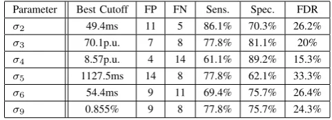
This is also confirmed by the results shown in Table II. Classification based onH2OM yelinW M alone resulted in a false discovery rate of 15.3% whereas the corresponding FDR of T1,GM was more than twice as high. The remaining parameters ranged between those extreme values. However, even though the FDR of some univariate classifiers are close to the FDR of the multivariate model, it has to be noticed that the number of falsely classified subjects is approx. 36% higher for the univariate classifier with the smallest number of misclassifications (H2OT otW M) as compared to the full multivariate model (15 vs. 11 misclassifications).
TABLE II
PERFORMANCE OF THE UNIVARIATE CLASSIFIERS
Parameter Best Cutoff FP FN Sens. Spec. FDR
σ2 49.4ms 11 5 86.1% 70.3% 26.2%
σ3 70.1p.u. 7 8 77.8% 81.1% 20%
σ4 8.57p.u. 4 14 61.1% 89.2% 15.3%
σ5 1127.5ms 14 8 77.8% 62.1% 33.3%
σ6 54.4ms 9 11 69.4% 75.7% 26.4%
σ9 0.855% 9 8 77.8% 75.7% 24.3%
IV. CONCLUSION
contains sufficient information for an accurate prediction of the presence of MS. Moreover, the features employed were very simple but robust at the same time. An increased classification performance might be expected by adding in-formation e.g. on the spatial heterogeneity of each parameter or higher-order histogram based features such as those used in [24] to predict age and gender using quantitative MRI. In contrast to the multivariate analysis, the evaluation of single parameters shows a lower classification performance with an increased number of falsely classified datapoints. Here again two white matter parameters, the total and myelin bound water content, resulted in the lowest error rates. This shows that normal appearing white matter of MS patients is already affected by the disease. Specifically, the average myelin water content is reduced whereas the total amount of water is increased at the same time. The first observation is a characteristic sign of demyelination whereas the latter is a strong surrogate marker for inflammation, where both processes are important in the pathogenesis and progression of mutliple sclerosis [1].
We have observed that the falsely classified subjects differed in age and gender from the corresponding cohort. Therefore, a future study should include more subjects and use age and gender as additional covariates to the classification model. Due to the relatively small number of subjects, such an analysis was not feasible here. Instead, age and gender matched groups were used to minimise a possible bias associated with these two phenotypes.
This work presents a first step towards a more comprehensive study of disease progression and effects of therapeutic inter-ventions in individual patients. The main goal of the current study was the proof-of-principle that a combination of super-vised learning and quantiative MRI data of normal appearing brain matter provides information about the disease that is not contained in conventional MRI images. As such, it forms the basis for future studies on the above mentioned aspects and might ultimately lead to the determination of biomarkers that allow for a much more accurate classification of individual MS patients and a closing of the gap between imaging and clinical findings.
ACKNOWLEDGMENT
The authors would like to thank Lena Heinle for revising the article.
REFERENCES
[1] E. Miller, “Multiple sclerosis,” Adv. Exp. Med. Biol., vol. 724, pp. 222–238, 2012.
[2] C. H. Polman, S. C. Reingold, G. Edan, M. Filippi, H. P. Hartung, L. Kappos, F. D. Lublin, L. M. Metz, H. F. McFarland, P. W. O’Connor, M. Sandberg-Wollheim, A. J. Thompson, B. G. Weinshenker, and J. S. Wolinsky, “Diagnostic criteria for multiple sclerosis: 2005 revisions to the ”McDonald Criteria”,”Ann. Neurol., vol. 58, no. 6, pp. 840–846, Dec 2005.
[3] R. Bakshi, A. J. Thompson, M. A. Rocca, D. Pelletier, V. Dousset, F. Barkhof, M. Inglese, C. R. Guttmann, M. A. Horsfield, and M. Fil-ippi, “MRI in multiple sclerosis: current status and future prospects,”
Lancet Neurol, vol. 7, no. 7, pp. 615–625, Jul 2008.
[4] A. Ceccarelli, R. Bakshi, and M. Neema, “MRI in multiple sclerosis: a review of the current literature,”Curr Opin Neurol, Jun 2012. [5] A. L. Liang, I. M. Vavasour, B. Madler, A. L. Traboulsee, D. J. Lang,
D. K. Li, A. L. Mackay, and C. Laule, “Short-term stability of T (1) and T (2) relaxation measures in multiple sclerosis normal appearing white matter,”J. Neurol., vol. 259, no. 6, pp. 1151–1158, Jun 2012.
[6] H. Vrenken, A. Seewann, D. L. Knol, C. H. Polman, F. Barkhof, and J. J. Geurts, “Diffusely abnormal white matter in progressive multiple sclerosis: in vivo quantitative MR imaging characterization and comparison between disease types,” AJNR Am J Neuroradiol, vol. 31, no. 3, pp. 541–548, Mar 2010.
[7] A. L. MacKay, I. M. Vavasour, A. Rauscher, S. H. Kolind, B. Madler, G. R. Moore, A. L. Traboulsee, D. K. Li, and C. Laule, “MR relaxation in multiple sclerosis,”Neuroimaging Clin. N. Am., vol. 19, no. 1, pp. 1–26, Feb 2009.
[8] F. Manfredonia, O. Ciccarelli, Z. Khaleeli, D. J. Tozer, J. Sastre-Garriga, D. H. Miller, and A. J. Thompson, “Normal-appearing brain t1 relaxation time predicts disability in early primary progressive multiple sclerosis,”Arch. Neurol., vol. 64, no. 3, pp. 411–415, Mar 2007. [9] K. Schmierer, C. A. Wheeler-Kingshott, P. A. Boulby, F. Scaravilli,
D. R. Altmann, G. J. Barker, P. S. Tofts, and D. H. Miller, “Diffusion tensor imaging of post mortem multiple sclerosis brain,”Neuroimage, vol. 35, no. 2, pp. 467–477, Apr 2007.
[10] K. Schmierer, D. J. Tozer, F. Scaravilli, D. R. Altmann, G. J. Barker, P. S. Tofts, and D. H. Miller, “Quantitative magnetization transfer imaging in postmortem multiple sclerosis brain,” J Magn Reson Imaging, vol. 26, no. 1, pp. 41–51, Jul 2007.
[11] H. Vrenken, S. A. Rombouts, P. J. Pouwels, and F. Barkhof, “Voxel-based analysis of quantitative T1 maps demonstrates that multiple sclerosis acts throughout the normal-appearing white matter,”AJNR Am J Neuroradiol, vol. 27, no. 4, pp. 868–874, Apr 2006.
[12] D. Tozer, A. Ramani, G. J. Barker, G. R. Davies, D. H. Miller, and P. S. Tofts, “Quantitative magnetization transfer mapping of bound protons in multiple sclerosis,”Magn Reson Med, vol. 50, no. 1, pp. 83–91, Jul 2003.
[13] C. Laule, I. M. Vavasour, G. R. Moore, J. Oger, D. K. Li, D. W. Paty, and A. L. MacKay, “Water content and myelin water fraction in multiple sclerosis. A T2 relaxation study,”J. Neurol., vol. 251, no. 3, pp. 284–293, Mar 2004.
[14] C. Laule, E. Leung, D. K. Lis, A. L. Traboulsee, D. W. Paty, A. L. MacKay, and G. R. Moore, “Myelin water imaging in multiple sclerosis: quantitative correlations with histopathology,”Mult. Scler., vol. 12, no. 6, pp. 747–753, Dec 2006.
[15] H. Neeb, K. Zilles, and N. Shah, “A new method for fast quantitative mapping of absolute water content in vivo,”Neuroimage, vol. 31, no. 3, pp. 1156–1168, Jul 2006.
[16] H. Neeb, V. Ermer, T. Stocker, and N. J. Shah, “Fast quantitative map-ping of absolute water content with full brain coverage,”Neuroimage, vol. 42, no. 3, pp. 1094–1109, Sep 2008.
[17] V. Tonkova, V. Arhelger, J. Schenk, and H. Neeb, “Rapid myelin water content mapping on clinical MR systems,”Z Med Phys, vol. 22, no. 2, pp. 133–142, Jun 2012.
[18] R. Mathur-De Vre, “Biomedical implications of the relaxation be-haviour of water related to NMR imaging,”Br J Radiol, vol. 57, no. 683, pp. 955–976, Nov 1984.
[19] H. Neeb. (2014, June) Professional Remagen Diagnostic Image Classification Tool for MS (predictM S). [Online].
Available: http://www.hs-koblenz.de/rac/fachbereiche/mut/forschung- projekte/labore-projekte/multimodal-imaging-physics/quantitative-mri-in-ms/predictms/
[20] N. J. Shah, H. Neeb, M. Zaitsev, S. Steinhoff, G. Kircheis, K. Amunts, D. Haussinger, and K. Zilles, “Quantitative T1 mapping of hepatic en-cephalopathy using magnetic resonance imaging,”Hepatology, vol. 38, no. 5, pp. 1219–1226, Nov 2003.
[21] N. J. Shah, H. Neeb, G. Kircheis, P. Engels, D. Haussinger, and K. Zilles, “Quantitative cerebral water content mapping in hepatic encephalopathy,”Neuroimage, vol. 41, no. 3, pp. 706–717, Jul 2008. [22] H. Neeb, J. Schenk, and B. Weber, “Multicentre absolute myelin
water content mapping: Development of a whole brain atlas and application to low-grade multiple sclerosis,” NeuroImage: Clinical, vol. 1, no. 1, pp. 121 – 130, 2012. [Online]. Available: http://www.sciencedirect.com/science/article/pii/S2213158212000186 [23] H. Neeb, “Dynamic modeling of nuclear fusion as a new tool to
iden-tify subgroups in multiple sclerosis magnetic resonance imaging data,”
Lecture Notes in Engineering and Computer Science: Proceedings of The World Congress on Engineering and Computer Science 2012, WCECS 2012, 24-26 October, 2012, San Francisco, USA, pp. 634– 639, Oct 2012.
[24] H. Neeb, K. Zilles, and N. J. Shah, “Fully-automated detection of cerebral water content changes: study of age- and gender-related H2O patterns with quantitative MRI,”Neuroimage, vol. 29, no. 3, pp. 910– 922, Feb 2006.
[25] R. O. Duda, P. E. Hart, and D. Stork,Pattern Classification. John Wiley and Sons, 2000.