Online Full Text

Abstractـــــ In Wireless Sensor Networks (WSN’s), it is imperative to utilize the most power efficient techniques to prolong the lifetime of a sensor node. Backpressure based scheduling has a remarkable performance for WSNs, and it has been discussed extensively in literatures. However, considering the energy efficiency of Backpressure scheduling algorithms for recourse-constrained WSNs is still need to be studied in order to design WSNs with minimum energy consumption. Unlike previous works for Backpressure scheduling algorithms, in this paper we propose a novel Multi-Factors Backpressure Scheduling (MFBS) algorithm which focuses on introducing new link-weights for energy efficient scheduling in WSNs. In MFBS, besides queue backlog differentials which is the common scheduling method in the classical Backpressure algorithm, nodal residual energy as well as the shortest path between neighbors (nodes) are also jointly considered into the transmission scheduling decision. Based on the results of our extensive simulation which is proven by the equivalent theoretical analysis, MFBS shows a significant improvement in the network performance of WSNs in terms of the network lifetime, the network throughput, the average queue length and the energy efficiency in comparison with existing algorithms such as the classical backpressure algorithm and enhanced dynamic backpressure routing algorithm.

Index Termsـــــ WSN scheduling, power consumption techniques, Backpressure algorithms, energy-efficient design of WSNs.

I. I

NE of the key challenges in wireless sensor design is energy efficiency, since the nodes have limited power resources as they typically operate off of batteries that are difficult to replace or recharge [1]. Therefore, a considerable amount of research in WSNs has focused on power saving techniques including the proposal of various power-efficient scheduling mechanisms (e.g. [2, 3]) and power-efficient Medium Access Control (MAC) protocols (e.g. [4, 5]). Recently, many researches have been made for implementation of backpressure scheduling algorithm in WSNs. Backpressure scheduling algorithm was first proposed in [6], and it has be proven by simulation and mathematical analysis to be optimal in term of the network performance. Some efforts of enhancing the backpressure scheduling algorithm focused on combining the algorithm with the rate control mechanisms in order to provide network-utility-optimal scheduling guarantee ( e.g. [7, 8]),

Manuscript received March 5, 2016; revised March 16, 2016. The work was supported by Taif University, Saudi Arabia.

The author is with the Computer Engineering Department, Taif University, P.O.Box : 888, Hawiyah, Taif, Zip Code : 21974, Saudi Arabia. Email:[email protected]

or combining the backpressure scheduling algorithm with the best rout selection in order to provide high packet delivery efficiency such as the works in [ 9,10].

In classical Backpressure algorithm, if the network has multiple links and in order to transmit packets it is required to activate some of non-interference links which leads to the maximum sum of link weight (i.e. the largest flow weight on the link) multiplying corresponding link rate. Here, the weight associated with a flow is the differential of the flow’s queue backlogs between the two endpoints of the link. In such transmission scheduling, network packets are always pushed from the networks hotspots without considering the transmission results. That is, if the transmission lead to routing detours or even loops. It is a fact that such classical backpressure scheduling mechanism enables packets to utilize the whole network capacity, and achieve adaptive resource allocation and support load-aware routing. However, the network latency may increase over long E2E between two nodes, and low network lifetime performance may be notified due to the lake of consideration of the energy efficiency when making the decision to rout the packet from one hop to the next [6].

Turning to using backpressure scheduling algorithm in WSNs, there are many efforts to enhance the algorithm to be useful in such networks. For example, authors in [11] proposed backpressure collection protocol (BCP) for WSNs, where forwarding decision to the next hop is made based on neighbors’ queue backlogs. BCP can achieve higher packet delivery ratio especially if there are queue hotspots around sink nodes. In other words, it is necessary to have stable queue backlog gradient among neighboring nodes. However, such stability doesn't exists all the time in WSNs where sensor nodes only inject packets into the network intermittently and that is only when they measure phenomena and need to send corresponding packets to the sink nodes. In addition, some other works focus on enhancing backpressure scheduling algorithm in WSNs such as [12] and [13], but all of these efforts still suffer from the lake of considering the energy use efficiency which is the main design issue need to be considered when proposing scheduling algorithms for WSNs.

Therefore, the work in this paper has been motivated and main contribution that we need to address in this paper is to propose a novel energy efficient multi-factors backpressure scheduling algorithm (MFBS) for WSNs. In MFBS, we introduce a new link's weight assignment method for the purpose of decision making when routing the packet from one hop to the next. MFBS is based on assigning two new factors for a link weight. That is the link's weight is not only based on the differential between its two endpoint nodes’ queue backlogs as the classical backpressure algorithm, but also two new factors which are the residual energy of the

A Novel Multi-Factors Backpressure Scheduling

Algorithm for Energy-Efficient Design of

Wireless Sensor Networks

Fawaz Alassery,

Member,IAENG

node as well as the shortest distance between two neighbor nodes will be considered. Thus, in MFBS, the network performance in term of increasing the lifetime of sensor nodes (i.e. increasing the energy efficiency) will be improved since the packet will be transmitted to the next hop that has more residual energy and shorter distance to the transmitting node. In addition, in MFBS, the packet delivery ratio as well as the network throughput will be improved in comparison with existing backpressure algorithms such as the classical backpressure algorithm and enhanced dynamic backpressure algorithm. To the best of our knowledge, the work presented in this paper is novel, and different from all previous efforts that enhanced the backpressure scheduling algorithm to be useful for limited energy resources networks such as WSNs.

The reminder of this paper is organized as follow. Section II describes our proposed system model. Section III defines our proposed multi-factors backpressure scheduling algorithm, and shows how to achieve the throughput optimality. In section IV, we evaluate the network performance of our proposed algorithm, and compare the energy efficiency, packet delivery ratio and the throughput of our algorithm against commonly used scheduling algorithms (e.g. the classical backpressure algorithm and enhanced dynamic backpressure algorithm). In section V, we conclude the paper.

II. SYSTEM MODEL DESCRIPTION

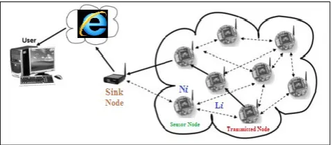
Figure 1 depicts an example of a WSN where a number of sensor nodes are deployed arbitrarily to perform certain functionalities including sensing and/or collecting data and then injecting packets into the network. All packets are assumed to be transmitted to only one destination (i.e. the sink node), and packets from a transmitter may take multiple hops before reaching the sink node. Routing, scheduling, and rate control can be done in each sensor node in the network independently. The sink node may process and relay the aggregate data to a backbone network. In addition, we assume the time dimension is slotted, so a sensor node will send its packets in its reserved time slot, which is denoted by t. In our design, we also assume that a WSNs can be modeled as a graph G=(N, L), where N represents the set of sensor nodes in the network and L represents the set of links.

Fig.1: Wireless Sensor Network (WSN) with N sensor nodes, L links and one sink node (receiver).

The queues in classical backpressure scheduling algorithm requires every node in G to maintain forwarding queue for the flow which is transmitted over the node. This per-flow queue backlog of flow x that is transmitted over the node at time slot t can be denoted by (t). At the beginning of each

time slot, the transmitted node will inject the external data traffic of each flow into the network. Based on [6], if

is the number of packets of flow x that is arrived at the queue of at flow f's transmitted node (i.e. s(x)), then the

dynamics of queue backlog of flow x can be represented as:

(t+1) = (t) + (1)

In addition, once the traffic arrives to the destination, it will leave the network layer which means that the queue backlogs will be equal to zero. This can be written as:

(t) = 0, for 0 (2)

Where, d(x) represent the flow arrives at the destination. Authors in [6], reached to the conclusion that the network stability for the dynamics of queues can be gained as long as all sensor nodes in G can achieve the following expression:

∑ [ ] (3)

The flows in WSNs are different from those considered in classical backpressure algorithm due to the fact that flows in WSNs aren't long-lived. Here, sensor nodes send their packets or stop sending at any time which is based on the occurrence of particular phenomena at specific palace. So, packets sent from all sensor nodes can be seen at one flow at the sink node, and the source of such flow is the node set which includes all sensor nodes in the network.

III. MULTI-FACTOR BACKPRESSURE SCHEDULING

ALGORITHM (MFBS)DESCRIPTION

As mentioned earlier, our proposed algorithm is based upon studying backpressure scheduling algorithm and proposing two new factors (i.e. sensor nodes residual energy and the shortest path for relaying packets) for the purpose of decision making when relaying packets from one hop to the next hop for all the path from the transmitter to the sink node. Thus, packets generated from one node will be transmitted to a neighbor node that has higher residual energy and a shorter distance to the transmitter. As a result, a remarkable power saving for sensor nodes will be gained and the network lifetime will be extended. In the following we illustrate how to introduce a new link weight when forwarding packets to the sink node.

Let's first show how the flows in WSNs can be modeled. As we described in section II, flows in WSNs aren't long-lived. Here, sensor nodes send their packets or stop sending at any time which is based on the occurrence of particular phenomena at specific palace. So, packets sent from all sensor nodes can be seen at one flow at the sink node, and the source of such flow is the node set which includes all sensor node un the network. Hence, the equation (1),(2) and (3) can be rewritten in the case of WSNs as follows:

The dynamics of queue backlog for a node Ni can be represented as:

(t+1) = (t) + (4) Where is the number of packets that arrive to the node

Ni. And similar to equation (2), the queue backlogs will be

equal to zero at the sink node:

Finally, the network stability for the dynamics of queues can be gained as long as all sensor nodes in G can achieve the following expression:

∑ [ ] (6)

In our algorithm, we introduce a new link weight. So, the queue length differential between to end nodes in the network for the classical backpressure algorithm [6] will not be the only factor need to be considered. The new link weight between to nodes x and y is expressed as:

+ (7)

Where is the differential of the queue length between the nodes x and y, is the factor that

represent the probability that node x selecting node y as the next hop for forwarding packets. The smaller probability of

means the link between x and y will not be chosen for

the next hop forwarding of packets. This is because the residual energy for the node y is low or it is located in a place that is not closer to the sink node. So, in our design, the selection of the next hop forwarding will be based on the residual energy of node y and the shortest distance between node x and the sink node or the node y to the sink node (e.g. node x may send a packet to the node y which has high residual energy but it has longer distance to the sink node than the transmitter (i.e. node x), so this link between x and y will have low as it is not the perfect choice for the

next hop forwarding.) Now let's define the probability factor

, if the next node (or node y) is the destination (i.e. the

sink node), then = ; where is a constant that we

can change every time during the simulation, is the distance factor for the node x to the sink node. However, if the next node (or node y) isn't the destination (i.e. not the sink node), then = ) + ; where is the

distance factor for the node y, is the residual energy for the node y which is equal to the initial energy of the node y divided by the current energy of the node y (i.e. =

.

Thus, our works in MFBS will not contradict with the throughput optimality of the classical backpressure scheduling algorithm. That is, all we try to achieve is to define a new link weight mechanism for the next hop forwarding, so links with lower weights (i.e. lower residual energy and located far away from the sink node) will be ignored. So the power will be saved since the two metrics (factors) that we take care of them are the routing based on finding the next hop (node) that have more residual energy and located in a coordination which is close to the sink node. Hence, in MFBS, if the link between node x and y is selected, then packets will be transmitted over this link (x,y) in its scheduled time frame (t), which can be defined as:

(t) = max [∑ ] (8)

Equation (8) is very similar to the optimization problem which is proposed in the classical backpressure scheduling algorithm [6], but the new link weight has been proposed as shown in equation (7). In order to get the optimal solution which leads to optimal schedule for equation (8), let's rewrite the equation (7) to include the bounded values of

factor as follows:

+ ) + (9)

Let's assume

=

for the node

x

in sending

state at time

t

, and

for node

y

in

receiving state at time

t

. So, we can rewrite equation

(9) as follows:

[ ] ( ) (10)

[

] (

)

In equation (11), it can be seen that at every time slot

t

for nodes

x

and

y

where

x,y

N

(

G

), then

=

=

O

(

| |

) (i.e. the

computational complexity) can hold based on [14],

where

N

is the number of all nodes in the networks.

Based on the proposed GMM scheme in [14], the

above computational complexity can be reduced to

O

(

| | | |

), where

L

IV. PERFORMANCE EVALUATION

In this section we provide extensive simulation for the performance evaluation of our proposed MFBS algorithm for various system design scenarios and parameter choices. Here, we compare the performance of our MFBS algorithm with the well-known classical backpressure algorithm the enhanced backpressure scheduling algorithm. The simulation parameters are explained in table 1.

As shown in the tale, we assume the sensing filed of 200 sensor nodes which distributed randomly (one of them is the rechargeable sink node which is located in the center of the sensing filed) is 300m 300m. Sensor nodes will inject their packets (the length of a packet is 1024 bits) into the network and all packets need to be delivered to the rechargeable sink node. Packets arrival rate follow Poisson distribution where = 0.2, 0,4, 0.6,0.8, 1.0, 1.2,1.4,1.6,1.8,2.0. We divide the time slots which are shared between sensor nodes into 600 slots.

In addition, in our simulation we use the first order radio model which represents the power consumption of WSNs nodes for transmitting, receiving and data aggregation as shown in figure 2. This radio model has been discussed extensively in literature (e.g. [15] and [16]). The first order radio model assumes asymmetric transmission. That is, the power required to transmit a message from node x to node y is the same power required to transmit the message form node y to node x for a given SNR. Based on the distance between a transmitter and a receiver, the first order radio model is divided into free space model and multipath fading model. For nodes which are close to each for a distance which is less than a pre-defined threshold level ( ), the

free space propagation model is used. On the other hand, for nodes which are located far away from each other for a distance which is greater than the threshold level ( ), then

the multipath fading model is used where the signals strength are affected by obstacles such as buildings or trees. In general, the respectivetransmission ( ) and reception

( ) energy consumption to transmit and receive l-bits

Fig.2: First order radio model used to simulate the power consumption if WSNs.

) = ) (12)

for free space model:

= ( ; if d <

for multipath fading model :

= ( ; if d >

) = (13)

=

In equations (12) and (13), is the energy consumption

for electronic circuits when transmitting l-bits message, is the energy consumption for data

aggregation at the transmitter, is the energy consumption

due to the amplifier for the free space model, is the

energy consumption due to the amplifier for the multipath fading model, is the energy consumption for electronic

circuits when receiving -bits message.

The performance parameters that are presented in this section are:

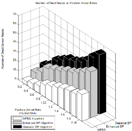
 The network lifetime: It is the time interval from the first packet being transmitted by a sensor node until the death of the last sensor node. It can be represented by showing the time of the first dead node, and the number of dead nodes starting from the beginning until the end of the simulation for all three compared algorithms (i.e. our MFBS and Classical BP and Enhanced BP algorithms).

 The Throughput: The throughput can be measured by calculating the number of packets that delivered successfully per time slot.

 The Average Queue Length: The queue length is another performance parameter which is considered in our analysis in order to illustrate how our proposed MFBS algorithm has lower queue length over different arrival rate.

 The Energy-Efficiency: The Energy-efficiency of a network is also considered in our analysis in order to illustrate the power consumption of sensor nodes over the simulation slots. Here, nodes which are marked as dead because of the expenditure of their energy will not be considered in the next transmission route.

Table 1: Summary of simulation parameters

Sensing field 300m 300m

Number of sensor nodes 200 The rechargeable sink

node location (150,150)

Number of nodes (N) 100 sensor nodes

Message size (l) 1024 bits

Number of slots 600 slots

Links capacity 1.00

SINR 4dB

Arrival rate ( ) 0.2,0.4,0.6,0.8,1.0,1.2, _{1.4,1.6,1.8,2.0}

Initial energy ( ) 0.5J

Energy for transmitter electronic circuit ( )

50 nJ/bit

Energy for transmitter data aggregation ( )

5 nJ/bit

Energy due to free space

model ( ) 5pJ/bit/

Energy due to multipath

fading path model ( ) 0.002 pJ/bit/

Energy for receiver electronic circuit ( )

50nJ/bit

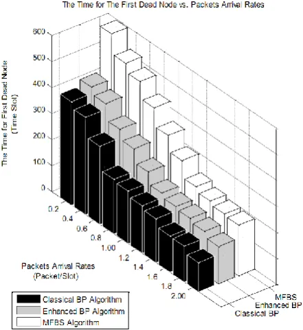
For the first performance parameter, which is the network lifetime, it can be shown in figure 3 that MFSB outperforms the classical BP and the enhanced BP algorithms especially when increasing the packets arrival rates. For example, in figure 3.a, if the packets arrival rate is 1.00, then the number of dead nodes of the MFBS algorithm is 16 nodes while the number of dead nodes at the same packet arrival rate for the enhanced BP and classical BP algorithms are 29 and 38, respectively. In figure 3.b, at all arrival rates = 0.2, 0.4, 0.6, 0.8,1.0, 1.2, 1.4, 1.6,1.8,2.0, it is obvious that the first dead node encountered at late time slots for the MFSB algorithm, while the first dead node for the classical BP and enhanced BP algorithms will be encountered at early time slots. Thus these figures (i.e. figure 3.a and figure 3.b) demonstrate how our proposed MFSB algorithm has a great impact on the network lifetime which will be extended remarkably.

Fig.3.b: Performance parameter 1: The time for the first dead node vs. packets arrival rates.

For the second performance parameter, it can be seen in figure 4 that the proposed MFBS algorithm outperforms both the classical BP and enhanced BP algorithms over all simulated arrival rates. For example, the throughput (Packets/slot) when the arrival rate ( )= 0.2 is 0.41 for the MFBS algorithm, while it is equal to 0.22 and 0.16 for the enhanced BP and classical BP algorithms, respectively. It is also seen that the throughput increase when increasing the packets arrival rates, the throughput for the proposed MFBS algorithm reach to 0.82 when the packets arrival rate ( )= 2.00. This increase in the network throughput is expected due to the fact that adaptive BP algorithms have ability to utilize the whole network capacity and use many alternative routes when delivering packets from sensor nodes to the rechargeable sink node.

Fig.4: Performance parameter 2: The network throughput vs. packets arrival rates.

For the third performance parameter, it is obvious that when increasing the packets arrival rates, the queue length will build up for all adaptive BP algorithms. However, because of the remarkable throughput of MFBS algorithm which is shown in figure 4, our proposed MFBS algorithm still provide better queue length which is lower than both the classical BP and the enhanced BP algorithms as shown in figure 5.

Fig.5: Performance parameter 3: The average packets length queue vs. packets arrival rates.

Finally, for the fourth performance parameter, figure 6 shows that the proposed MFBS has better energy efficiency in comparison with the classical BP and the enhanced BP algorithms over all simulation slots which is assumed to be 600 slots.

Fig.6: Performance parameter 4: The energy-efficiency vs. number of time slots.

V. CONCLUSION

we defined new link weight factors which are based on routing packets from one node to its neighbor based on finding the node that has higher remaining energy and the shortest distance to the receiver sink node. We showed the theoretical representation of MFBS and studied its performance in terms of the network lifetime, the throughput, the average queue length and the energy-efficiency. From the extensive simulation results we reach to the conclusion that our proposed MFBS algorithm achieves better performance than the classical BP and the enhanced BP algorithms without violating the optimality of backpressure algorithms. The simulation results are demonstrated in figures and tabulated in tables which allows a system designer multiple degrees of freedom for design trade-offs and optimization.

REFERENCES

[1] M. Khanafer, M. Guennoun, and H. T. Mouftah, “A survey of beacon enabled IEEE 802.15.4 MAC protocols in wireless sensor networks,” IEEE Commun. Surveys Tuts., vol. 16, no. 2, pp. 856–876, Second Quarter 2014.

[2] Tong, F.; Zhang, R.; Pan, J., "One Handshake Can Achieve More: An Energy-Efficient, Practical Pipelined Data Collection for Duty-Cycled Sensor Networks," in Sensors Journal, IEEE , vol.PP, no.99, pp.1-1

[3] Gong, S.; Duan, L.; Gautam, N., "Optimal Scheduling and Beamforming in Relay Networks With Energy Harvesting Constraints," in Wireless Communications, IEEE Transactions on , vol.15, no.2, pp.1226-1238, Feb. 2016 [4] Alvi, A.N.; Bouk, S.H.; Ahmed, S.H.; Yaqub, M.A.; Sarkar,

M.; Song, H., "BEST-MAC: Bitmap-assisted Efficient and Scalable TDMA based WSN MAC protocol for Smart Cities," in Access, IEEE , vol.PP, no.99, pp.1-1

[5] Zheng, T.; Gidlund, M.; Akerberg, J., "WirArb: A New MAC Protocol for Time Critical Industrial Wireless Sensor Network Applications," in Sensors Journal, IEEE , vol.16, no.7, pp.2127-2139, April1, 2016

[6] L. Tassiulas and A. Ephremides, “Stability properties of constrained queueing systems and scheduling policies for maximum throughput in multihop radio networks,” IEEE Transactions on Automatic Control,vol.37,no.12,pp.1936– 1948,1992.

[7] M. Neely, E.Modiano, and C. Li, “Fairness and optimal stochastic controfor heterogeneous networks,” in Proc. IEEE INFOCOM’05, pp. 1723–1734, Mar. 2005.

[8] L. Georgiadis, M. J. Neely, and L. Tassiulas, “Resource allocation and cross-layer control in wireless networks”, Now Publishers Inc, 2006.

[9] S. Moeller, A. Sridharan, B. Krishnamachari, and O. Gnawali, “Routing without routes: The backpressure collection protocol,” in Proc. IEEE/ACM IPSN’10, pp. 279–290, Apr. 2010.

[10][7] H. Seferoglu and E. Modiano, “Diff-Max: Separation of routing and scheduling in backpressure-based wireless networks,” in Proc. IEEE INFOCOM’13, pp. 1555-1563, Apr. 2013.

[11]S. Moeller, A. Sridharan, B. Krishnamachari, and O. Gnawali, “Routing without routes: The backpressure collection protocol,” in Proc. IEEE/ACM IPSN’10, pp. 279–290, Apr. 2010.

[12]Z.Jiao,Z.Yao,B.Zhang,andC.Li,“A Distributed gradient assisted any cast-based backpressure framework for wireless sensor networks,” in Proceedings of the 1st IEEE International Conference on Communications (ICC ’14),pp.2809–2814,Sydney, Australia, June 2014.

[13]Z. Jiao, B. Zhang, W. Gong, and H. Mouftah, “Virtual queue based back-pressure scheduling algorithm for wireless sensor networks,” EURASIP Journal on Wireless Communications and Networking,vol.2015,no.35,2015

[14]X.LinandN.B.Shroff,“Theimpactofimperfectschedulingon cross-layer congestion control in wireless networks,” IEEE/ACMTransactions on Networking,vol.14,no.2,pp.302– 315,2006.

[15]D.Heinzelman, W. Rabiner, A. Chandrakasan, and H. Balakrishnan.“ Energy-efficient communication protocol for wireless micro sensor networks.” System Sciences, 2000. Proceedings of the 33rd Annual Hawaii International Conference on. IEEE, 2000.