Optimization of tillage and sowing operations using discrete event simulation

Optimization of tillage and sowing operations using

discrete event simulation

Armaghan Kosari Moghaddam, Hassan Sadrnia*, Hassan Aghel,

Mohammad Bannayan

Faculty of Agriculture, Ferdowsi University of Mashhad, Mashhad, Iran

Abstract

Kosari Moghaddam A., Sadrnia H., Aghel H., Mohammad B. (2018): Optimization of tillage and sowing operations using discrete event simulation. Res. Agr. Eng., 64: 187–194.

A simulation model was developed for secondary tillage and sowing operations in autumn, using discrete event simulation

technique in Arena® _{simulation software (Version 14). Eight machinery sets were evaluated on a 50-hectare farm. Total}

costs including fixed-costs, variable costs and timeliness costs were calculated for each machinery set. Timeliness costs were estimated for 21-years period on daily basis (Daily Work method) and compared with another method (Average Work method) based on the equation proposed by ASAE Standards, EP 496.3FEB2006. The Inputs of the model were machinery sets, field size, machines performances and daily soil workability state. The optimization criteria were the lowest costs and lowest standard deviation in daily work method plus the lowest costs based on average work method. The validity of the model was evaluated by comparing the output of the model with field observed data collected from various farms. Results revealed that there was no significant difference (P > 0.01) between the observed and predicted finish day.

Keywords: discrete event simulation; modeling, sowing; tillage, timeliness costs

The costs of ownership and operating of farm ma-chinery were almost the largest part of production costs. Therefore, development or selection of the optimal machinery systems could help to reduce the costs. In addition, providing timely field operations will help to optimize the yield and its quality (Rotz, Harrigan 2005). A logical selection of farm ma-chinery consists of four segments included system power requirement, tractor-implement combina-tion, field-machine matching and cost analysis (Ogunlowo 1997). One of the most important fac-tors in machinery selection procedure is cost analy-sis. So we have to define a criterion for choosing an optimum machinery set through economic aspect. For a given farm, the “appropriate” machinery set in economic terms would be the “least-cost” set when specific machinery, labor and timeliness costs are considered” (de Toro, Hansson 2004).

these programs are based on discrete event simula-tion technique. This modeling technique provides simulation of daily field operations on a farm con-sidering available resources (machinery, labour), constraints (e.g. soil workability) and management criteria. This technique may also allow estimation of timeliness costs and their variations with better accuracy than those methods working with single values of workdays (de Toro, Hansson 2004).

There are a lot of studies that have used simulation modeling for agricultural production costs man-agement and optimizing the selection procedure of farm machinery however there are a few studies that have considered timeliness costs. Most of ap-proaches and tools that have determined timeliness costs, used methods based on international or local standards and only reported these costs based on average of various years. The aim of this study was to implement the discrete event simulation method for determining timeliness costs based on daily basis and comparing it with conventional method (Aver-age work method) based on ASAE standards.

MATERIAL AND METHODS

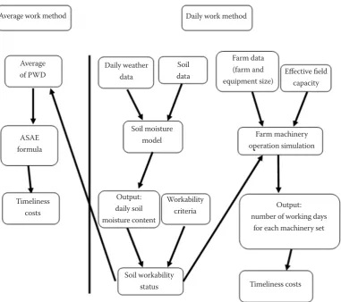
A simulation model for farm machinery opera-tions was developed using discrete event simulation technique. Inputs of the model are soil workability state, farm size, machinery sets and field capacity of each machine. The general trend of simulation processes similar to de Toro and Hansson (2004) is outlined in Fig. 1.

Estimation of working days. A soil moisture

model was developed (Kosari Moghaddam 2014) and was run using 21-years (1992–2012) weather data from a meteorological station of Mashhad and soil characteristics of Research Station of Fer-dowsi University of Mashhad (36°15'N/59°36'E) (Koocheki et al. 2011). The soil texture of this farm was loam type and field capacity was estimated 210 mm, similar to other loam soils in this location (Bannayan et al. 2011). Workdays were estimated for autumn using two workability criteria namely daily soil moisture less or equal to 85% field capac-ity (de Toro, Hansson 2004) and daily

precipita-Fig. 1. Schematic representation of two methods (daily work method and average work method) for determination of timeliness costs (de Toro, Hansson 2004)

Average work method

Average

of PWD Daily weather _data dataSoil

Farm data (farm and

equipment size) Effective field _capacity

ASAE formula

Timeliness costs

Output: daily soil moisture content

Workability

criteria _{number of working days}Output: for each machinery set Soil moisture

model _{operation simulation}Farm machinery Daily work method

Timeliness costs Soil workability

tion less than 4 mm (local surveys). The output of this model was used as input of daily work method and probability of workdays in complete periods were used as input of average work method.

Simulation of farm machinery operations. Farm

machinery operations were simulated using dis-crete event simulation technique in Arena®

simu-lation software (Rockwell Automation, Version 14, Milwaukee, USA) with two following sub-models namely workdays and farm machinery operation. The computational experiments were performed on an Intel Pentium T4400 CPU2.2 GHz worksta-tion. In workdays sub-model, a "day" that should be assessed for working day arrives as an "entity" at "create" module and then is transferred to "Read/ Write" module that is assign "working day" attribute based on soil model output spreadsheets and then is gone to "Decide" module. If the day is workable, is transferred to "Signal" module and number 1 send to "Hold" module in farm machinery sub-model. Otherwise, that day is considered as non-workable

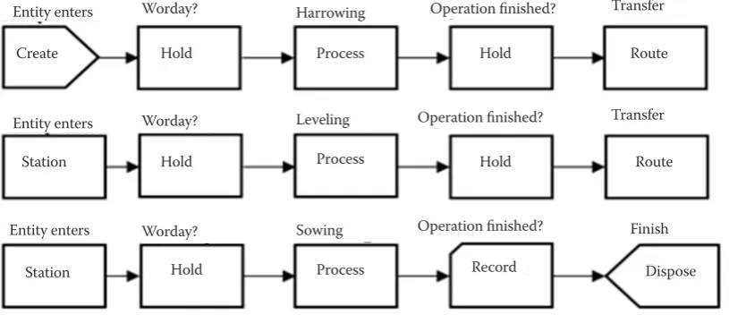
and "Dispose" from model. An auxiliary "Decide" module is considered to specify "finish time" to this sub-model. A simplified sketch of this sub-model is shown in Fig. 2. In Farm machinery operation sub-model, each hectare of field to be ploughed, enters as "Entity" to "Create" module with specific time steps and then is send to "Hold" module for determining working day. When the day is workable, the entity can go to "Process" module for each operation. Each machinery set was considered as "Resource" and each operation was considered as individual "Pro-cess" module. Afterwards, entity is transferred to "Hold" module for determining finish operation. If the operation is finished or accomplished to some extent, the entity is transferred to next "Station" by means of "Route" module, in expect of "Sowing Operation". A simplified sketch of this sub-model is shown in Fig.  3. Model was started at first day of autumn 1992 and repeated for 21-years period (1992–2012). The priority of operations was harrow-ing, leveling and sowharrow-ing, respectively.

Fig. 2. A simplified sketch of workdays sub-model

Fig. 3. A simplified sketch of farm machinery operation sub-model

Entity enters

Entity enters

Entity enters

Worday?

Worday?

Worday?

Harrowing

Leveling

Sowing

Operation finished?

Operation finished?

Operation finished?

Transfer

Transfer

Finish Create

Station

Station

Hold

Hold

Hold

Hold

Hold

Record _Dispose Route

Route Process

Process

Process

Create Read/Write Decide Decide Entity enters Read from Excel file

Operation

finished? Working day? Go to farm machinery _sub-model

Yes Yes

No No

Dispose

Dispose

Signal _Dispose

Finish

Finish

Simulation of machinery operations. Common

machinery operations were secondary tillage (har-rowing and leveling) and sowing for wheat produc-tion in autumn. Eight machinery sets (C1-C8) were selected based on availability in this region (Table 1). The differences between these sets were the number and working width of tillage equipment and the num-ber of tractors. All sets used the same planter to re-move the effects of working conditions of sowing op-eration. These operations were simulated for 21-years period (1992–2012) using the simulation model on a 50-hectare “virtual” farm in Mashhad. Field capacity for each machine and working hours were consid-ered 0.67 ha·h–1 _{for harrow-1, leveler and planter and}

1.07 ha·h–1 _{for harrow-2 based on Research Station of}

Ferdowsi University of Mashhad.

Costs estimation. When the finish day for each

set was determined according to the output of the simulation model, total cost of each set was cal-culated using Microsoft Excel 2007 Spreadsheets. This cost includes fixed cost, variable costs and timeliness cost. Fixed costs were depreciation, an-nual interest rate, taxes, insurance and housing for tractors and equipment but insurance was not considered for equipment. Depreciation costs were calculated based on ASAE Standard ED 230.3 for

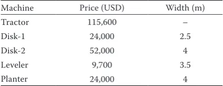
first year. Purchase prices were given from online farm machinery sales websites and were presented in Table 2. Salvage value (S) and machine life (L) for tractors and equipment were 20% purchase price, 13 and 7 years, respectively based on Ministry of Agriculture statistics (www.amar.org.ir) of 2014. Interest rate (I) was considered 6% and taxes, in-surance and housing were assumed 1%, 0.25% and 0.75% of purchase price.

Variable costs were included fuel, oil and lubrica-tion, repair and maintenance, tire and driver costs for tractors and repair costs for equipment. Fuel cost was calculated according to Eq. (1):

F = Hr × 0.308 PTO_maxPTO (1)

where: Hr – annual working hours for tractor (h);

PTO_maxPTO – max. power in PTO (kW)

Gasoline cost per liter was 0.07 dollars. In this study, tractors were ITM 399 (Iran Tractor Manu-facturing Company, Tabriz-Iran). PTO_maxPTO was 70 kW based on product catalogue. Lubrication and maintenance costs were considered about 20–25% fuel cost. Repair and tire costs were assumed 10 and 4% of purchase price and driver wage was 2 dollars per hour (Ministry of Agriculture (Iran) 2014).

The timeliness costs were calculated for sowing operation considering the effect of land preparation operation on sowing start day. So, it was varied based on last day of tillage operation. Moreover, the effect froze/freeze damage was negligible because all sow-ing periods were selected accordsow-ing to the conditions of this region. These costs were calculated based on two following methods. In average work method, timeliness costs were calculated using the following equation Eq. (2) proposed by ASAE Standards (EP 496.3 FEB2006) for sowing operations in autumn:

TC= K×A2×Y×V

Z×G×C_i×(pwd) (2)

where: TC – timeliness costs (dollars); K – timeliness coef-ficient; A – area (ha) that was considered 50 hectares in this study; Y – average yield per area for wheat (ton.ha-1_); V – value per yield (dollars·.ton-1_{); Z – four if the}

opera-tion can be balanced evenly about the optimum time, and should be two if the operation either commences or terminates at the optimum time; C_i – machine capacity (ha·h–1_{); G – expected time available for field work each}

day (h); pwd – probability of a working day (decimal)

Timeliness coeficcient K was 0.005, average yield was determined 9.5 t·ha–1 _{and optimum sowing day} Table 1. Machinery sets characteristics for simulating

farm machinery operations

Set Number of equipment _{of tractors}Number Disk-1 Disk-2 Leveler-1 Planter

C1 1 – 1 1 1

C2 1 – 1 1 2

C3 1 – 1 1 3

C4 2 – 1 1 3

C5 2 – 2 1 5

C6 – 1 1 1 1

C7 – 1 1 1 2

C8 – 2 1 1 3

Table 2. Purchase price of tractors and equipment for fixed-costs calculations

Machine Price (USD) Width (m) Tractor 115,600 – Disk-1 24,000 2.5

Disk-2 52,000 4

Leveler 9,700 3.5

was considered October 12th _{based on the study}

of Nazeri et al. (2010). Yield value was 0.36 dol-lars per kilogram (Statistical Center of Iran 2014). Working hours per day was also considered fixed as 7.5 h based upon actual farming practices of the Research Station of Ferdowsi University of Mash-had. This value can be changed based on manager decision. Moreover, Z value was 2 for all sets C2 and C3 and pwd was calculated 0.85 for all sets ex-cept C1 that was calculated 0.84.

In daily work method, annual yield losses were calculated based on Eq. (3) that was modified form of Eq. (2) (de Toro 2005):

Y_i= P_d × A × (D_s – D_o) + 0.5 × P_d × A × (D_f – D_s) (3)

where: Y_i – annual yield losses for sowing operation (kg);

P_d – daily penalty (kg·ha–1_·day–1_{); D}

s – the start day for operation (day number); D_o – optimum day for opera-tion (day number); D_f – finish day for operation (day number); A – field area (ha)

If D_f< D_o, annual yield losses were equal to zero and if D_s < D_o and D_f > D_o, D_s was equal to D_o(de Toro 2005). According to Nazeri et al. (2010), P_d was determined as 48.8 kg. Start day was consid-ered 23th _{September and timeliness costs were}

cal-culated by Eq. (4):

TC = Y_i × V (4)

Validation. The output of the simulation model

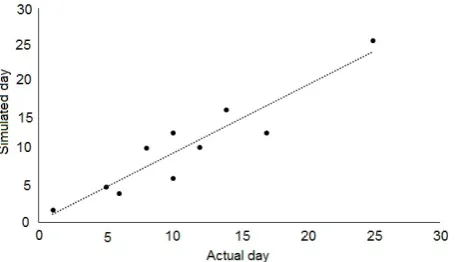
was finish day of each operation and subsequent-ly the length of operation for each machinery set. These results were verified with 10 different farm sizes (between 3–40 ha) during 9 years (2002– 2010). Data gathered from farm included field size, machinery set, operational conditions and start and finish days for every operation in each given

farm. The simulation model was run under these conditions and the results (the length of each op-eration) were compared with actual length of that farm operation with t-test in SPSS 16 at 5% prob-ability level. Results were shown in Fig. 4. Results obtained from t-test showed that there was no sig-nificant difference between simulated and actual farms and the correlation coefficient was 0.935.

Sensitivity Analysis. The analysis was performed

to measure the sensitivity of selecting the optimum set to changes in field size. For this purpose, field size was changed to 25 and 75-hectare and other parameters were not changed, then simulation model was run, and finish day of each operation was recorded. Finally, the total costs of each set were calculated using spreadsheets and the opti-mum set was found for every field size.

RESULTS AND DISCUSSION

Cost estimation of machinery sets

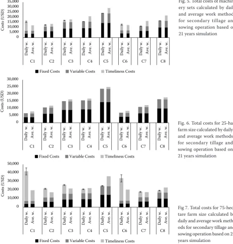
Fixed, variable and timeliness costs for both daily and average work methods and also standard de-viations for daily work method are shown in Fig. 5. The results showed that total costs were close to each other for C1, C6 and C7 sets. This was due to distribution pattern of costs that the large part of costs was related to timeliness costs in C1 and C6 sets and fixed and variable costs in C7 set. Finally, C1 and C7 sets were selected as optimum sets based on average work method and daily work method, respectively. Based on these results, costs of farm machdepended on distribution of fixed, variable and timeliness costs. So if a small set was selected, fixed and variable costs were low but timeliness cost was high while in a large set, fixed and variable costs were high and timeliness cost was low.

Sensitivity analysis of model

Results of simulation model for 25 and 75-hec-tare farms were shown in Figs 6 and 7. Timeli-ness costs due to early crop establishment were not considered in daily work method, and then total costs were larger in C4, C5 and C8 sets for average work method compared to daily work method in the 25-hectare farm. In this farm, the smallest set – C1 – was the optimum set in both methods (Fig. 6).

Fig. 5. Total costs of machin-ery sets calculated by daily and average work methods for secondary tillage and sowing operation based on 21 years simulation

Fig. 6. Total costs for 25-ha farm size calculated by daily and average work methods for secondary tillage and sowing operation based on 21 years simulation

Fig 7. Total costs for 75-hec-tare farm size calculated by daily and average work meth-ods for secondary tillage and sowing operation based on 21 years simulation 0 5,000 10,000 15,000 20,000 25,000 30,000 35,000 Daily w . Ave. w . Daily w . Ave. w . Daily w . Ave. w . Daily w . Ave. w . Daily w . Ave. w . Daily w . Ave. w . Daily w . Ave. w . Daily w . Ave. w .

C1 C2 C3 C4 C5 C6 C7 C8

Costs

(USD)

Fixed Costs Variable Costs Timeliness Costs

0 5,000 10,000 15,000 20,000 25,000 30,000 Daily w . A ve . w . Daily w . A ve . w . Daily w . A ve . w . Daily w . A ve . w . Daily w . A ve . w . Daily w . A ve . w . Daily w . A ve . w . Daily w . A ve . w .

C1 C2 C3 C4 C5 C6 C7 C8

Costs

(USD)

Fixed Costs Variable Costs Timeliness Costs

0 10,000 20,000 30,000 40,000 50,000 Daily w . Ave. w . Daily w . Ave. w . Daily w . Ave. w . Daily w . Ave. w . Daily w . Ave. w . Daily w . Ave. w . Daily w . Ave. w . Daily w . Ave. w .

C1 C2 C3 C4 C5 C6 C7 C8

Costs

(USD)

Fixed Costs Variable Costs Timeliness Costs

tal costs for C1 and C6 sets were larger in daily work method, because when the number of working days were increased, probability of working days were de-creased in the 75-hectare farm. In this farm, the C7 set was the optimum set in both methods (Fig. 7). As the results of model showed, when farm size increased, timeliness costs increased and this was due to con-fluence to bad weather conditions in late periods so farm machinery size should be increased. Rotz et al. (1983) showed that as the farm size was increased from 200 to 400 ha, sizes of machinery sets were in-creased by 30% to 40%. Haffar and Khouri (1992)

presented that as farm size was increased from 14 to 56 ha, the annual costs increased by 330%. Gunnars-son and HansGunnars-son (2004) also illustrated that increas-ing organic farm size, increased the farm machinery requirement for sowing and harvesting.

Effect of farm size to cost per hectare

were relatively equal for 50 and 75-hectare farms and in the other sets this relationship was not confirmed because of excessive timeliness costs for 75-hectare farm. This illustrated that these sets were not suitable for 75-hectare farm due to excessive timeliness costs. In average work method, except of C1 and C6, cost per hectare decreased when farm size increased. In C1 and C6 sets, excessive timeliness costs causing in-creasing in total costs and then cost per hectare due to not adequate capacity of them. In Rotz et al. (1983) study was shown that costs per hectare will decreased when farm size increased due to higher efficiency of farm machinery in large farms.

Comparison of daily and average work methods

In daily work method, since the output of model should finish every day of each operation and also given the start day, it is possible to determine time-liness costs based on daily basis, whereas in average work method, these costs are calculated for entire pe-riod. Moreover, using discrete event simulation needs to have detailed daily weather data, while only prob-ability of working days was needed for average work method. Timeliness costs for early crop establishment was not considered in daily work method however suitable management policies could compensated it.

CONCLUSION

In this study a simulation model for secondary tillage and sowing operations was developed by

employing discrete event simulation using Arena language. The outputs of model were completion dates of secondary tillage and sowing operations, so timeliness costs could be determined for a series of years on a daily basis. These findings were com-pared with results from the Average work method. Generally, the main conclusions are:

There was no significant difference between simu-lation model output and observed data in farm and present model showed an acceptable performance.

Daily work method requires more data compared with average work method, and its results are more detailed and comprehensive. Moreover, in compari-son with daily work method, average work method was not enabled to considered climate uncertainty among studied years. It could be more highlighted in areas with higher annual weather variation. Total costs depend on distribution of fixed, variable and timeliness costs. Thus, smaller machinery sets can have lower fixed and variable and higher timeliness costs.

If detailed historical data are available, the appli-cation of simulation techniques for farm machinery management could be used as a suitable tool for de-termination of total costs (fixed, variable and timeli-ness costs) and optimization of them.

Acknowledgments

The authors would like to appreciate the Research Station of Ferdowsi University of Mashhad for pro-viding the required data. We also like to thank Pro-fessor Alfredo de Toro for his valuable comments that greatly improved this manuscript.

Fig. 8. Costs per hectare for 25, 50 and 75-hectare farm calcu-lated by daily and average work methods for secondary tillage and sowing operation based on 21 years simulation

0 200 400 600 800 1,000 1,200

C1 C2 C3 C4 C5 C6 C7 C8

C

os

ts p

er

h

ec

ta

r

(U

SD

)

Machinery sets

25-hectar(daily w.)

50-hectar(daily w.)

75-hectar(daily w.)

25-hectar(aver.w.)

50-hectar(aver. w.)

References

Al-Hamed S. A., Al-Janobi A. A. (2001): An object-oriented program to predict tractor and machine system perfor-mance. Research Bulletin, King Saud University, 106: 5–24. ASAE (2006): Agricultural Machinery Management ASAE

EP496.3.

Bannayan M., Lakzian A., Gorbanzadeh N., Roshani A. (2011): Variability of growing season indices in northeast of Iran. Theoretical and Applied Climatology, 105: 485–494. Camarena E.A., Gracia C., Sixto J.M.C. (2004): A mixed in-teger linear programming machinery selection model for multifarm systems. Biosystems Engineering, 87: 145–154. Dash R.C., Sirohi N.P.S. (2008): A computer model to select

optimum size of farm power and machinery for paddy-wheat crop rotation in Northern India. Agricultural Engi-neering International: the CIGR Ejournal: 12.

Gunnarsson C., Hansson P.-A. (2004): Optimisation of field machinery for an arable farm converting to organic farm-ing. Agricultural Systems, 80: 85–103.

Haffar I., Khoury R. (1992): A computer model for field ma-chinery selection under multiple cropping. Computers and Electronics in Agriculture, 7: 219–229.

Koocheki A., Shabahng J., Khorramdel S., Azimi R., Aghel H. (2011): Documentation of farming management with GIS and ArcView: A case study for agricultural Research Station of Faculty of Agriculture, Ferdowsi University of Mashhad, Iran. Journal of Iranian Field Crop Research, 6: 909–919. (in Farsi). Kosari Moghaddam A. (2014): Optimization of tillage

ma-chinery selection in grain farms using discrete event simu-lation.[ Master’s Thesis.] Ferdowsi University of Mashhad (Iran) (in Farsi). Abstract available on http://thesis.um.ac. ir/moreinfo-56053-pg-1.html

Ministry of Agriculture (Iran) (2014): Agricultural Jihad Machinery Development Center. Estimation of Tariff of Mechanization Services in Iran.

Nazeri M.A., Abadi A. Z.F., Koohestani B., Mirak T.N. (2010): Investigation on the response of different wheat types in suitable and delayed sowing day in Mashhad climatic conditions. 11th Iranian Crop Science congress. Envi-ronmental Sciences Research Institute, Shahid Beheshti University, Tehran. (in Farsi).

Ogunlowo A.S. (1997): Machinery selection based on gross-margin costing analysis: a case Study of Abeokuta local government aeras in Nigeria. West Indian Journal of Engineering: 40–48.

Rotz C.A., Harrigan T.M. (2005): Predicting suitable days for field machinery operations in a whole farm simulation. Applied Engineering in Agriculture, 21: 10.

Rotz C.A., Muthar H.A., Black J.R. (1983): A multiple crop machinery selection algorithm. Transaction of ASAE: 1644–1649.

Sahu R.K., Raheman H. (2008): A decision support system on matching and field performance prediction of tractor-implement system. Computers and Electronics in Agri-culture, 60: 76–86.

Søgaard H.T., Sørensen C.G. (2004): A model for optimal selection of machinery sizes within the farm machinery system. Biosystems Engineering, 89: 13–28.

Statistical Center of Iran. (2014): Agricultural services costs and products prices. Available at http://www.amar.org.ir/ Portals/0/Files/reports/1393/g_ghmvhkhk_93.pdf (in Farsi). de Toro A. (2005): Influences on timeliness costs and their vari-ability on arable farms. Biosystems Engineering, 92: 1–13. de Toro A., Hansson P.-A. (2004): Analysis of field machinery

performance based on daily soil workability state using dis-crete event simulation or on average workday probability. Agricultural Systems, 24: 109–129.