Development and use of simulation models in Operational Research: a comparison of discrete event simulation and system dynamics

(1)

University of Warwick institutional repository: http://go.warwick.ac.uk/wrap

A Thesis Submitted for the Degree of PhD at the University of Warwick

http://go.warwick.ac.uk/wrap/2984

This thesis is made available online and is protected by original copyright. Please scroll down to view the document itself.

(2)

Development and use of simulation

models in Operational Research: a

comparison of discrete-event simulation

and system dynamics

by

Antuela Anthi Tako

A thesis submitted in partial fulfilment of the

requirements for the degree of

Doctor of Philosophy

University of Warwick, Warwick Business School

(3)

Table of contents

Figures

Figure 1-1: Process flow diagram of a simple bank system, where customers arrive, wait in the queue, are served at the till and then leave the system (adapted from

Robinson, 2004). ... 5

Figure 1-2: Information/action/consequences loop, based on (Coyle, 1996). ... 12

Figure 2-1: Simulation of a harvested fishery with stepwise changes in fleet size (Morecroft and Robinson, 2005) ... 42

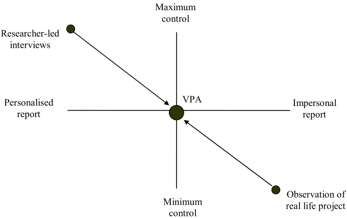
Figure 3-1: Configuration of methods by level of personalisation of reports and researcher control on data collection process. ... 72

Figure 4-1: Graphical representation of the historical & projected UK prison population size. ... 86

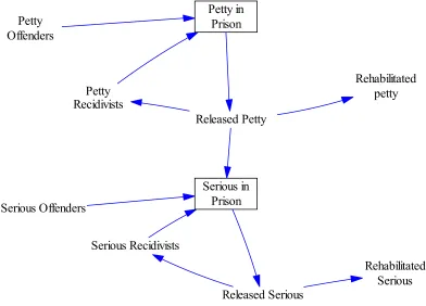
Figure 4-2: Graphical representation of prison system for the model building sessions. ... 89

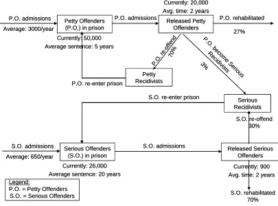
Figure 4-3: Graphical representation of the flow of prisoners in the model use case. ... 90

Figure 5-1: Number of words verbalised and modelling time for 5 DES and 5 SD modellers. ... 106

Figure 5-2: Speed of words verbalised per minute by the 5 DES and 5 SD modellers. ... 107

Figure 6-1: Correlation of the amount of verbalisation with length of modelling experience of the participant sample. ... 125

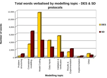
Figure 6-2: Total number of words verbalised by 5 DES and 5 SD modellers by modelling topic. ... 127

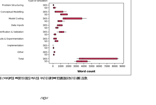
Figure 6-3: Box and whiskers plot of DES and SD modellers’ verbalisations by modelling topic. ... 130

Figure 6-4: Example of data verbalisations on problem structuring, illustrating how M, the greatest vertical difference is identified. ... 132

Figure 6-5: Average percentage of attention paid to the 7 modelling topics by DES and SD modellers. ... 134

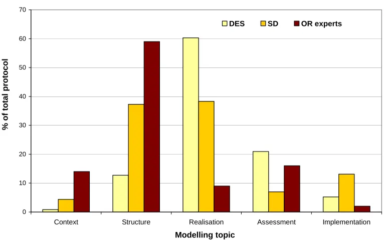
Figure 6-6: Comparing the distribution of attention to 5 modelling topics for DES, SD and Willemain’s OR experts. ... 137

Figure 6-7: Timeline plots for DES1and DES5 verbalisations. ... 141

Figure 6-8: Timeline plots for SD1 and SD4 verbalisations. ... 142

Figure 6-9: SD modelling as an iterative process (Sterman, 2000, pp. 87) ... 146

Figure 6-10: Key stages in DES modelling, as an iterative process, with verification & validation in the centre (Robinson, 2004). ... 147

Figure 6-11: Comparative view of the transition matrices for the combined DES and SD protocols, where each cell has been colour-coded depending on the number of transitions. ... 148

(8)

Figures

Figure 9-1: Feedback effects in the prison system ... 279

Figure 9-2: Process Flow Diagram - DES prison model ... 282

Figure 9-3: DES model representation in Witness, with the model on the left-hand side, input criteria in the top box on the right and in the box below model outputs. ... 283

Figure 9-4: DES model outputs ... 284

Figure 9-5: Causal loop diagram – SD prison model ... 286

Figure 9-6: SD model representation in Powersim. ... 287

Figure 9-7: SD model Control Panel, which included the user interface and model results page. This was the main working environment. ... 288

Figure 10-1: P-P plot on understanding of the relationship between variables, SD vs. DES answers, where 1 means understand very little and 5 understand very well. 312 Figure 10-2: P-P plot on understanding of how to use the model, SD vs. DES answers, where 1 means understand very little and 5 understand very well. Points 1 & 2 coincide with the origin of the coordinates (0, 0) because none of the respondents answered with: understand very little, and little, for either model. ... 313

Figure 10-3: Frequency diagram showing importance of animation and paper-based description as factors that helped user understanding of the model (DES & SD) . 314 Figure 10-4: P-P plot on level of detail of the model, SD vs. DES answers, where 1 means very detailed and 5 meant very high level. ... 316

Figure 10-5: P-P plot on model representativeness, SD vs. DES answers, where 1 means very little and 5 very much. Points 4 and 5 coincide because none of the respondents considered the models representative at level 5. ... 319

Figure 10-6: P-P plot on the capacity of the model to facilitate the communication of ideas, SD vs. DES answers, where 1 means very little and 5 very well. ... 320

(9)

Tables

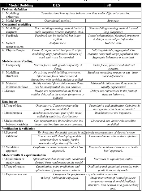
Table 2-1: Fundamental differences between DES and SD. ... 27

Table 2-2: Taxonomy of model structures (Brennan et al., 2006) ... 55

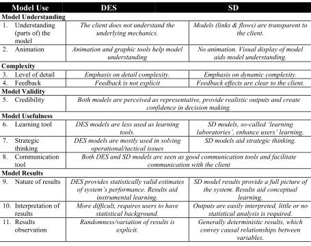
Table 2-3: Summary of comparison literature on DES and SD approach to model building. ... 58

Table 2-4: Summary of comparison literature on DES & SD modelling philosophy. ... 59

Table 2-5: Summary of comparison literature on the use of DES and SD models. . 59

Table 3-1: Hypotheses 1.1 – 1.3 on the comparison of the DES and SD model building process. ... 65

Table 3-2: Hypotheses 2.1 – 2.18 on the comparison of the DES and SD model building approach. ... 65

Table 3-3: Hypotheses 3.1 – 3.6 on the comparison of DES and SD modelling from the users’ point of view ... 68

Table 4-1: Initial assumptions/numbers suggested in the case study for model building sessions. ... 89

Table 5-1: Non testable and factual research hypotheses not verified in the study 117 Table 6-1: List of DES and SD modellers’ profiles ... 122

Table 6-2: DES and SD participants tabulated in groups of experience by software used. ... 123

Table 6-3: Average number of words and fraction of the standard deviation/mean calculated for each modelling topic for DES and SD protocols. ... 128

Table 6-4: The results of the Kolmogorov-Smirnov test comparing the DES and SD modellers’ verbalisations for 7 modelling topics and the total protocols. The significant differences are highlighted, based on the comparison of the greater vertical distance M to the critical value =0.8. ... 132

Table 6-5: DES and SD modellers’ verbalisations (number of words and proportion of attention) by modelling topic. ... 135

Table 6-6: Total number of transitions per linear strip in the DES and SD transition matrices ... 152

Table 7-1: Verification & Validation – division into two categories comparing the DES and SD modellers’ verbalisations (number of words and proportions) on verification & white-box validation and black-box validation ... 228

Table 7-2: Count of the times the keywords “equilibrium”, “steady state”, “stable” or “steady” appear in the 5 SD protocols. ... 234

Table 7-3: Type of results referred to by DES modellers ... 236

Table 7-4: Type of results referred to by SD modellers ... 238

Table 7-5: Scenarios considered by DES and SD modellers ... 240

(10)

Tables

Table 9-2: Comparison of DES and SD models outputs. ... 292

Table 9-3: Determining questions to be asked ... 294

Table 10-1: Sample representation by industry sector ... 307

Table 10-2: Sample representation by functional area ... 308

Table 10-3: Managerial level for each group ... 309

Table 10-4: Prior experience by management level (includes both DES and SD samples) ... 309

Table 10-5: Ranking of factors that helped user understanding of the models (DES & SD) ... 314

Table 10-6: Results from answers on type of outputs DES & SD users refer to when running the model ... 323

Table 10-7: Comparison of answers to open-ended question about the observation of trends in the graphs ... 325

(11)

Acknowledgements

I am indebted to many people for the help, advice and support provided during the process of completing this PhD thesis. I would like to dedicate this work to my mother, who has always given me the inspiration and the craving for learning. She has been and will always be my motivator in pursuit of knowledge.

Firstly, I would like to thank my supervisor, Professor Stewart Robinson for the continuous encouragement, support and guidance. I am extremely grateful for his direction and timely advice that has enlightened me throughout the process of compiling this work. I also appreciate the comments and the help provided by Professor Ruth Davies, my second supervisor. Thanks must also go to both my examiners, John Morecroft and Frances O’Brein, for having patiently read the thesis and for giving me constructive feedback.

(12)

Acknowledgements

Thanks must go to the participants of the two studies involved in this work. Even though their names are kept anonymous, I feel indebted to the expert simulation modellers who took the time to participate in the model building study. I now enjoy a good rapport with most of the participants, usually meeting with them in various conferences. I am also grateful to Dr. Susan Howick for her help in contacting potential participants. I would also like to thank the 2 groups of Executive MBA students for participating and completing the questionnaire survey involved in the model use study. Thanks go to the administrative staff at the Executive MBA programme at Warwick Business School, Karen Finlay and Irene Ioannou for their help and support with the preparations of materials for the model use sessions.

I would also like to thank Lanner Group for their help with using Witness.

I am also grateful for the various sources of funding which have enabled me to attend conferences which allowed me to gain a valuable insight into OR. These include: Operational Research and Management Sciences Group at Warwick, Warwick Business School, the UK OR Society, the International System Dynamics Society and the UK chapter of the System Dynamics Society.

(13)

Acknowledgements

secretaries of the Operational Research and Management Sciences group, Sue Shaw and Racheal Monnington for the animated chats and their support.

(14)

Declaration of authorship

I, Antuela Anthi Tako, declare that this thesis entitled:

“Development and use of simulation models in Operational Research: a comparison of discrete-event simulation and system dynamics” and the work presented are my own. I confirm that:

- This work was done wholly while in candidature for this research degree; - This thesis contains no material which has been accepted for the award of

any other degree or diploma in any university;

- I have acknowledged all main sources of help;

- The work described in this thesis has served the material for several published papers and conference presentations which are listed below.

Journal paper:

Tako A.A. & Robinson S. (2009) “Comparing discrete-event simulation and system dynamics: Users’ perceptions” Journal of the Operational Research Society, 60, (296-312), doi:10.1057/palgrave.jors.2602566.

Refereed conference proceedings:

“Model building in System Dynamics and Discrete-event Simulation: a quantitative comparison”, In the proceedings of the 26th International Conference of the System Dynamics Society, 20-24 July 2008, Athens, Greece. (The paper won the

(15)

Declaration of authorship

“Comparison of Model Building in Discrete-Event Simulation and System Dynamics”. In the proceedings of the 2008 OR Society Simulation Workshop (SW08), 1-2 April 2008, pp. 209-218, Worcestershire, UK.

“Towards an empirical comparison of DES and SD in the supply chain context”. In the proceedings of the 2006 OR Society Simulation Workshop (SW06), 28-29 March 2006, pp. 149-156, Leamington Spa, UK.

Conferences and presentations:

Presentation: “Comparing the Use of Discrete-Event Simulation and System

Dynamics Models”, PhD Colloquium in the Joint meeting of UK Chapter of the System Dynamics Society & OR Society SD+ Study Group, 7-8 February 2008, London South Bank University, London.

Workshop presentation: “Comparing SD & DES using prison population models”, in the Joint meeting of UK Chapter of the System Dynamics Society & OR Society SD+ Study Group, 7-8 February 2008, London South Bank University, London.

Poster presentation: “Comparing the Use of Discrete-Event Simulation and System Dynamics Models”, Winter Simulation Conference 2007, Washington D.C., 8-10 December 2007.

Presentation: “Discrete-Event Simulation & System Dynamics Models: Comparison from Users Point of View”, OR49 conference, OR Society, Edinburgh, 4-6

September 2007.

Presentation “Comparison of Discrete-Event Simulation and System Dynamics” at

Young OR15 conference (YOR15), OR Society, Bath, 28-30 March 2007.

(16)

Abstract

The thesis presents a comparison study of the two most established simulation approaches in Operational Research, Discrete-Event Simulation (DES) and System Dynamics (SD). The aim of the research implemented is to provide an empirical view of the differences and similarities between DES and SD, in terms of model building and model use. More specifically, the main objectives of this work are:

1. To determine how different the modelling process followed by DES and SD modellers is.

2. To establish the differences and similarities in the modelling approach taken by DES and SD modellers in each stage of simulation modelling.

3. To assess how different DES and SD models of an equivalent problem are from the users’ point of view.

In line with the 3 research objectives, two separate studies are implemented: a model building study based on the first and second research objectives and a model use study, dealing with the third research objective. In the former study, Verbal Protocol Analysis is used, where expert DES and SD modellers are asked to ‘think aloud’ while developing simulation models. In the model use study a questionnaire survey with managers (executive MBA students) is implemented, where participants are requested to provide opinions about two equivalent DES and SD models.

The model building study suggests that DES and SD modelling are different regarding the model building process and the stages followed. Considering the approach taken to modelling, some similarities are found in DES and SD modellers’ approach to problem structuring, data inputs, validation & verification. Meanwhile, the modellers’ approach to conceptual modelling, model coding, data inputs and model results is considered different. The model use study does not identify many significant differences in the users’ opinions regarding the specific DES and SD models used, implying that from the user’s point of view the type of simulation approach used makes little difference if any.

The work described in this thesis is the first of its kind. It provides an understanding of the DES and SD simulation approaches in terms of the differences and

similarities involved. The key contribution of this study is that it provides empirical evidence on the differences and similarities between DES and SD from the model building and model use point of view. Albeit the study does not provide a

(17)

Chapter 1

1. Chapter 1: Introduction

1.1 Introduction

This chapter introduces the topic of the thesis, setting the background of the work undertaken in the chapters to follow. For the readers who are not knowledgeable about simulation modelling, the discrete-event simulation and the system dynamics approach are initially described. A brief description of the thesis follows, which provides the reasoning behind and the initial thoughts that stimulated this study. This chapter ends with an overview of the chapters of the thesis.

1.2 What is simulation?

Talking about simulation as a tool in management science, Pidd (2003) explains that computer simulation is the use of a model to understand and experiment with a system. He also adds that a simulation model mimics the changes that occur through time in the real system. A more complete definition of simulation modelling is given by Robinson (2004), according to which simulation is the “experimentation with a simplified imitation (on a computer) of a […] system as it progresses through

(18)

Chapter 1

specific objective. The notion of simulation modelling in discrete-event simulation (DES) and system dynamics (SD) is fairly represented by the aforementioned definitions. A similar definition of SD modelling is given by Wolstenholme (1990), who defines SD as the study of the behaviour of physical and social systems over time through the creation of diagrammatic representations and computer simulations with the objective to understand system behaviour and to facilitate the design of the improved system. Therefore, when mentioning simulation throughout this thesis, both DES and SD are implied.

(19)

Chapter 1

The next distinction of simulation models, that of discrete and continuous systems is based on how time is handled in the system (Banks et al., 2001; Law, 2007). In discrete systems, state variables change in distinct time-steps (Δt) (i.e. the number of customers in a bank), while in a continuous system state variables change continuously (i.e. the amount of water flowing through a pipe). However, only few systems are completely discrete or completely continuous. For most systems one type of change predominates and it is therefore, possible to classify systems as either discrete or continuous based on the type of change that predominates (Banks et al., 2001; Pidd, 2004; Law, 2007). Hence, the decision as to the most suitable simulation approach to model a specific system varies.

Discrete-Event Simulation (DES) and System Dynamics (SD) are two popular simulation approaches used in Operational Research (Pidd, 2004). They are commonly used in business settings to support management learning and decision-making (Robinson, 2004). With these in mind, the two simulation approaches studied in this thesis, DES and SD are introduced in the next two sections.

1.3 Discrete-event simulation (DES)

(20)

Chapter 1

1.3.1 What is DES?

DES involves modelling of systems which consist of discrete entities going through specific states, which change at discrete points in time (Pidd, 2003). These points in time are the ones at which state changes (or events) occur. For example, if

customers arrive in a bank system at time 0, 3, 5, 8 and 11 then the model will progress by the corresponding time steps (Δt), 3, 2, 3 and 3.

(21)

Chapter 1

customer leaving the till) and so on. This illustrates how the simulation clock advances at unequal time slots, whenever an event occurs. Delay times in the form of periods of inactivity are also involved, which are skipped as the simulation clock jumps from one event time to another. An example of delay times is that of

customers waiting in the queue to be served.

Figure 1-1: Process flow diagram of a simple bank system, where customers arrive, wait in the

queue, are served at the till and then leave the system (adapted from Robinson, 2004).

The explanations provided in this section consist only of the basic principles involved in the logic of a DES model. For a more in-depth description of the

internal simulation logic the reader is referred to simulation textbooks (Banks et al., 2001; Pidd, 2004; Robinson, 2004; Law, 2007).

1.3.2 Main DES concepts

Entities are objects or components whose behaviour is tracked through the model as the simulation proceeds. Some examples of entities are: customers, patients and products. Entities go through a number of states, which represent their progression in the system. For example, in a bank customers go through a series of states: enter

Cashier Queue

Customer

(22)

Chapter 1

entity remains in a state for a period of time and whenever its state changes, an

event occurs. Events can be endogenous, i.e. to describe events that occur within the system (i.e. completion of a service) or exogenous to describe events in the

environment that affect the system (i.e. arrival of customers). Entities are given

attributes, which can be thought of as properties of each specific entity. Attributes are attached to the entities and these control various aspects such as: routing of objects, priority given to a customer waiting to be served, etc.

Activities are another important element in DES models. An activity takes a specific amount of time, which involves the time needed for an entity to change from one state to another. Typical activities include service times, inter-arrival times, or any other processing times defined in the simulation. In the bank example, an activity occurs throughout the time that the customer is in the ‘being served by the cashier’ state. An activity begins with an event and ends with an event. In the bank example, an activity occurs when a customer reaches the cashier (event 1) until they leave the system (event 2).

(23)

Chapter 1

following activity. However, conditional queues (or delays1) can also be specified, in which the progress of the entity through the process pauses until some simulated time interval has elapsed (Pidd, 2004).

A simulation control program maintains an event calendar which holds information regarding the state of all the entities in the system. This control program has a list of future events, ordered by time of occurrence. Every time an event occurs the

simulation control programme is updated with the current state of entities and also the time left for the entities to remain in a specific state.

From the point of view of DES modelling, most systems contain one or more sources of randomness. Therefore, a central aspect of DES simulation is the

inclusion of randomness or variability, from which DES gains its stochastic nature. Randomness is achieved with the use of random variables as inputs and sampling using random numbers. Random numbers consist of a sequence of numbers, integer or real, which appear in a random order. They are generated by a specific method2 and then used to determine the value of simulation variables from the probability function of empirical or statistical distributions. Two types of distributions are usually used discrete (binomial, Poisson, Bernoulli, etc.) or continuous (i.e.

exponential, gamma, uniform, etc.) distributions. For example, in a DES model of a bank typical random variables would be: customer arrivals and service times,

(24)

Chapter 1

represented by exponential and gamma distribution respectively. In stochastic models, outputs are presented as statistical estimates of the true system outputs, i.e. average number of customers waiting or average of customer waiting time, etc.

1.3.3 Evolution and applications of DES

The beginnings and evolution of the field of DES is related to the availability and developments in computing (Pidd, 2003; Pidd, 2004; Robinson, 2005). In the late 1950s and in the 1960s the first simulation models were developed in the form of computer code (Robinson, 2005). Later on, with the introduction of programming languages and more powerful computers, specialist simulation software were developed in the 1960s i.e. GPSS, SIMSCRIPT and SIMULA. At the same time, advances in simulation methodology were made with Tocher’s (1963) introduction to the three-phase approach in DES, which is still used by various DES packages.

(25)

Chapter 1

day and age, VIS is a common feature of most DES software. However, this was a breakthrough step at that time. This advancement was of course enabled with the rapid progress of computing and the spread of microcomputers. The first

commercial VIS software, SEE-WHY was developed in 1979, followed by other packages such as WITNESS, GENETIK, ProModel, etc.

In the 1990s further development of VIS continued, which consisted mainly of improvements in the software interface. Besides expensive simulation packages (WITNESS, Arena, Taylor II, AweSim, etc.), low cost packages were developed, Simul8, Extend, etc., which made simulation modelling more accessible to the wider user base. Some further developments in DES are: simulation optimisation, virtual reality, software integration and parallel distributed simulation (Robinson, 2005). Simulation optimisation became a significant feature in simulation, where the most commonly used optimisation approaches are: metamodelling, neural networks and metaheuristics. A number of simulation packages now incorporate some form of optimisation facility.

(26)

Chapter 1

users can interact with a gaming simulation model, models and software can be shared among distributed users, running model replications or scenarios across a number of distributed computers, etc. (Robinson, 2005).

DES has been traditionally used in the manufacturing sector, however, from the 1990s onwards it has been increasingly used in the service sector (Robinson, 2005). Some key DES applications include airports, call centres, fast food restaurants, banks, health care and business processes. Even though the developments of computing have to a great extent affected developments in DES modelling, Robinson raises awareness about the problems it can incur, including the

development of large and complex problems, with a knock on effect on the quality of the models. A lack of a wider methodology of DES modelling has also been pointed out (Robinson, 2005).

1.4 System dynamics (SD)

In the following paragraphs, a brief overview of the field of SD is provided, starting with the key concepts in SD modelling, followed by the applications and the

evolution of the field.

1.4.1 What is SD?

SD is a simulation approach with roots from engineering, cybernetics and

(27)

Chapter 1

behaviour and consequently to experiment with policies which will improve their behaviour. As its name implies, system dynamics studies dynamic behaviour of complex systems over time. The main interest of system dynamicists is the general dynamic tendency of the system as a whole, whether it is stable or unstable,

oscillating, growing or declining (Meadows, 1980). Hence, SD is considered to be taking a holistic, systems’ approach (Wolstenholme, 1990).

(28)

Chapter 1

Consequences (workforce level)

Action (Recruitment/ layoffs) Information (perceived

workforce level)

Figure 1-2: Information/action/consequences loop, based on (Coyle, 1996).

(29)

Chapter 1

competitors leave the market. Thus the number of competitors reduces, up to a point that the price reaches an equilibrium state.

Nonlinear relationships are an important feature in SD, which can affect the strength of feedback loops depending on the state of the system (Meadows, 1980; Sterman, 2000). In more complex models, the existence of several nonlinear relationships can result in a complex dynamic behaviour, which is more difficult to conceptualise and humans lack the cognitive ability to deduce the resulting dynamic behaviour

(Sterman, 2000). Therefore, computer simulation is considered necessary in order to deduce the system behaviour (Lane, 2000).

1.4.2 SD simulation concepts

(30)

Chapter 1

model, whereas information flows are not conserved, for example resources such as motivation are not limited in quantity.

In SD modelling two stages can be distinguished: qualitative and quantitative modelling (Wolstenholme, 1990; Coyle, 1996). Qualitative modelling involves building diagrams or conceptual models as a means of transmitting mental models, without necessarily using a computer. A number of tools are available such as: model boundary diagrams, sub-system diagrams, causal loop diagrams and stock and flow maps (Sterman, 2000). The latter 2 are the diagramming tools most often used in SD modelling.

Causal loop diagrams represent the feedback structure of the system using causal relationships between variables, starting from the cause and ending in the effect variable. Based on the type of effect, a positive or negative relationship between two variables can be determined. Stock and flow diagrams are a continuation of causal loop diagrams, where the physical processes occurring in the system are specified. Stock and flow diagrams represent the accumulation of resources into stocks, controlled by the flow rates (in-flows and out-flows) in the system, which may depend on information from auxiliary variables and other levels.

(31)

Chapter 1

over a period of time. SD is categorised as a continuous approach because the changes in the accumulated level are represented as continuous flows of material. The accumulated level served by a rate variable is equal to the area under the graph of the rate plotted over that period of time (Coyle, 1996). The progress of time in SD is based on advancement of the clock in equal small time-steps, called Δt, known as the ‘simulation’ interval. When building SD equation models, three points of time are of interest, the current point in time, the past point in time and the future point in time, all separated by the simulation interval (Δt).

1.4.3 Evolution and applications of system dynamics

Like DES, the field of SD came into being and evolved with the advent of

(32)

Chapter 1

(Hieber and Hartel, 2003). Forrester applied the SD approach in the social aspect and the problems involved in his subsequent studies of Urban Dynamics and World Dynamics. The main aspects involved are: population density, availability of jobs, migration and availability of housing.

The late 70s see a reduction in the number of SD applications, covering a wider range of academic disciplines, looking mainly at socio-economic problems

(Wolstenholme, 1990). At the same time, there has been a growing trend in moving away from quantified simulation models towards the qualitative (diagramming) approach. In the light of this, SD has been widely used to study ill-defined problems, forming epistemological and ontological assumptions that support the view that SD share common characteristics with soft systems methodology (Wolstenholme, 1990; Lane and Oliva, 1998). A significant advancement in the 80s was the emergence of user-friendly simulation software with advanced graphical user interfaces (STELLA, Powersim and Vensim) and the use of interactive simulation games (Forrester, 2007). From then onwards, applications of SD modelling have significantly expanded.

(33)

Chapter 1

1.5 What the thesis is about?

Practitioners and academics often get into discussions about which simulation approach is most suitable for modelling which problem. The choice between the two simulation approaches in practice is an on-going problem, however, in order to reach informed answers, a common understanding of the two simulation schools is needed. The current work contributes towards this aspect, looking into the

differences and similarities between DES and SD. Hence, the main research question that drives the work undertaken in the thesis is: “What are the differences and similarities between the DES and SD modelling approaches and the use of DES and SD models?”

In this thesis it is accepted that there are fundamental differences between DES and SD, which are derived from the technical concepts behind each simulation approach. It can be acknowledged that the two simulation techniques take different viewpoints to modelling and problem-solving. Whilst one might suppose that this makes them natural antagonists it can be argued that they complement each other (Morecroft and Robinson, 2005). Due to the limited literature and the lack of objectivity in the comparison criteria expressed in the literature so far, the scope of the thesis is to provide an empirical comparison of the two simulation approaches. More

(34)

Chapter 1

during the use of equivalent simulation models. The three main objectives of the thesis are:

1. To determine how different the modelling process followed by DES and SD modellers is.

2. To establish the differences and similarities in the modelling approach taken by DES and SD modellers in each stage of simulation modelling.

3. To assess how different DES and SD models of an equivalent problem are from the users’ point of view.

(35)

Chapter 1

Traditionally, since the beginnings of each field, there has been very little dialogue between the two modelling communities (Sweetser, 1999; Lane, 2000; Borshchev and Filippov, 2004; Morecroft and Robinson, 2005). Most recently some efforts are being made to create a bridge between the two simulation approaches. This is evidenced by the fact that a number of simulation experts from one area are attempting to enter into the other world. Furthermore the number of research projects3 currently under way reveals the increased interest shown in the

comparison of the two simulation approaches. This thesis also contributes towards this aspect, by representing the two worldviews and looking into how they can benefit from each other. Furthermore, DES and SD models of the same problem are developed.

1.6 Thesis outline

The rest of this thesis is organised in the following chapters.

3_{Herbert Daly, ‘Investigating Multi Method Modelling by Critical Comparison’, Brunel University;}

Jennifer Morgan, ‘Linking Discrete Event Simulation and System Dynamics in Healthcare’, University of Strathclyde (EPSRC case award);

EPSRC grant: ‘Multi-level simulation models (combining system dynamics and discrete-event simulation) for integrated strategic/operational modelling of health systems’, University of Southampton (EP/C531930/1);

(36)

Chapter 1

Chapter 2 introduces the existing literature on the comparison of the two simulation paradigms, discrete-event simulation (DES) and system dynamics (SD). The chapter discusses the key aspects considered in the comparison literature from the model building, modelling philosophy and model use point of view. A list of the key statements found in the literature is provided and conclusions are drawn with the view to specifying the objectives of the research undertaken.

Chapter 3 sets the scene for the empirical work undertaken in the thesis. The research question is discussed followed by the 3 key research objectives. The research hypotheses, based on the existing comparison literature are stated for the two different aspects of the comparison work undertaken, model building and model use. Furthermore, the research methodology is considered. The methods chosen for the model building and model use study, verbal protocol analysis (VPA) and survey questionnaire respectively, are explained.

In chapter 4, a case study on the UK prison population is presented. This case study serves as the research stimulus for both parts of the work undertaken and the

reasons for and the suitability of using it are discussed.

(37)

Chapter 1

process. An account of the pilot study implemented and the learning achieved is also provided.

The results of the quantitative analysis of the 10 verbal protocols derived from the model building study are presented in chapter 6. The aim of this chapter is to explore the differences and similarities in the DES and SD modelling process regarding the distribution of modellers’ attention to modelling topics and the sequence of attention among topics.

The results of the qualitative analysis of the 10 verbal protocols are provided in

chapter 7. The analysis is based on the testable research hypotheses stated in chapter 3. Thus DES and SD modellers’ thoughts relevant to the topic of each hypothesis are first presented followed by a comparison of the views expressed by the two groups of modellers. The findings from the quantitative and qualitative analysis (chapters 6 and 7 respectively), are further discussed in chapter 8.

Chapter 9 describes the study of model use based on the users’ perceptions of two equivalent DES and SD models. More specifically this chapter includes a

(38)

Chapter 1

(39)

Chapter 2

2 Chapter 2: A comparison of DES and SD in the literature

2.1 Introduction

In this chapter work on the comparison of two simulation approaches DES and SD is reviewed. The aim of this chapter is to provide an overview of the main issues discussed in the literature. The statements found in the comparison literature are considered with a view to specifying the aspects of DES and SD modelling to be investigated in the thesis.

The chapter starts with some general comments on the existing comparison literature, followed with a brief consideration of the technical differences between the two approaches. Then a list of the topics considered in the comparison literature is provided based on the aspects involved in the OR modelling process. Work on the choice of modelling approaches is also presented. The chapter ends with an overall summary of the topics considered in the comparison literature.

2.2 Overview of the comparison literature

(40)

Chapter 2

communication has been pointed out (Lane, 2000). In recent years, there has been some change with more academics and practitioners showing an interest in future collaboration between the two fields (Morecroft and Robinson, 2005). Therefore, the need for a comparative study is becoming more necessary.

Literature on the comparison of simulation approaches is scarce, consisting mainly of conference papers, which are not always publicly accessible. Work on the comparison of the two simulation techniques consists mostly of generally accepted statements (Brailsford and Hilton, 2001; Morecroft and Robinson, 2005). It mainly consists of authors’ personal opinions, which tend to be biased towards either the DES or SD approach, coming from their own area of expertise (Brailsford and Hilton, 2001). Furthermore, limited empirical work has been done to provide evidence certifying the existing statements in the literature. The only empirical study carried out to date is that of Morecroft and Robinson (2005). The authors built a step-by-step simulation model of a fishery, using SD (Morecroft) and DES

(Robinson) modelling, comparing model representation and interpretation. However, one could claim the existence of bias, as the two modellers were aware of each other’s views while creating their respective models.

(41)

Chapter 2

Rabelo, et al., 2005; Helal, et al., 2007). However, the technical differences between DES and SD modelling need to be acknowledged. These differences result from the underlying principles of each simulation approach and are briefly considered in section 2.3.

Literature on the comparison of DES and SD is distinguished in three main types of studies:

- Comparison of DES and SD models (Mak, 1993; Taylor and Lane, 1998; Sweetser, 1999; Lane, 2000; Brailsford and Hilton, 2001; Morecroft and Robinson, 2005).

- Combined use of DES and SD (Usano, et al., 1996; Petropoulakis and Giacomini, 1998; Music and Matko, 1999; Martin and Raffo, 2000; Donzelli and Iazeolla, 2001; Lee et al., 2002a; Lee et al., 2002b; Lakey, 2003;

Stchedroff and Cheng, 2003; Venkateswaran and Son, 2004; Greasley, 2005; Rabelo et al., 2005; Helal et al., 2007). The main areas of applications are: software development, manufacturing and production and supply chain.

(42)

Chapter 2

Work on the combined use of DES and SD is increasingly growing and emphasis is given on the complementary use of the two simulation approaches, where each one can be used to represent different aspects of the problem studied.

2.3 Technical differences between DES and SD

While an introduction to the DES and SD approach has already been provided in chapter 1, in this section the key technical differences between the two approaches are pointed out (Table 2-1).

DES views systems as a network of queues and activities, where state changes occur at discrete points of time. Whereas in SD, models are viewed as a system of stocks and flows where continuous state changes occur over time. In DES entities are individually represented and can be tracked through the system. Specific attributes are assigned to each entity, determining what happens to them throughout the simulation. On the other hand, in SD entities are represented as a continuous quantity, and are ‘indistinguishable’. Specific entities cannot be followed throughout the system.

(43)

Chapter 2

between the accuracy of the differential equations of the system versus the cost of computer time (Coyle, 1985). Furthermore, Coyle points out that time, as a variable is differently handled in the two modelling approaches. In DES time is usually incorporated as an implicit variable, which is usually of no direct interest to the modeller, while in SD modelling time is an explicit variable of direct interest (ibid). However, it can be argued that this depends on the specific problem situation modelled.

The underlying mathematics used in the equivalent simulation software differs. In DES, the underlying mathematics is part of the software language, of which the user has little understanding. SD models are based on differential equations

approximated in discrete time slices, which are entered by the modeller as part of the model building process. DES models are stochastic in nature with randomness incorporated through the use of statistical distributions. SD models are generally deterministic and variables usually represent average values.

Despite the above differences, it is claimed that the objective of models in both simulation approaches is to understand the way systems behave over time and to compare their performance under different conditions (Sweetser, 1999).

Table 2-1: Fundamental differences between DES and SD.

Fundamental differences DES SD

System representation Queues & activities Stocks & flows

State changes Discrete Continuous

(44)

Chapter 2

2.4 A taxonomy of topics considered in the comparison literature

After having discussed the fundamental differences between DES and SD, this section provides a review of existing comparison work, based on the specific issues raised in the literature. This section aims to represent the opinions expressed in the literature about DES and SD. These opinions are built around the model building process and the use of the respective simulation approaches in practice. The review of the existing comparison work is structured based on the aspects involved in the OR modelling process. Before exploring the specific topics found in the comparison literature regarding how the two simulation approaches compare, the stages of the OR model building process are identified as well as some general aspects regarding the simulation modelling process (sub-section 2.4.1). Then the comparison literature by modelling stage is discussed in the relevant sections (2.5 - 2.11), as well as the choice of simulation approach (section 2.12).

2.4.1 The model building process in DES and SD

The stages followed in generic OR modelling consist of the following (Hillier and Lieberman, 1990; Oral and Kettani, 1993; Willemain, 1995):

(45)

Chapter 2

- Model validity

- Model results and experimentation - Implementation and learning

In the respective DES and SD textbooks, teaching the art of simulation modelling, the steps suggested are equivalent to the stages followed during OR modelling, similar to the list provided above. This implies that both DES and SD modelling follow similar modelling stages.

Regarding the model building process followed, it is mentioned that in DES modelling emphasis is given in the development of the model on the computer (model coding). Baines et al. (1998) completed an experimental study of various modelling techniques, among others DES and SD, and their ability to evaluate manufacturing strategies. The authors commented on the time taken in building the DES model. The time taken in model building was considerably longer compared to SD and other modelling techniques. Furthermore, Artamonov (2002) developed two equivalent DES and SD models of the beer distribution game model and

commented on the difficulty involved in coding the model on the computer. He found the development of the model on the computer more difficult in the case of the DES approach, whereas, the development of the SD model was less troublesome. One possible explanation given by Baines et al (1998) is the fact that DES

(46)

Chapter 2

compared to the other techniques, which consequently results in a more detailed and complex model.

On the other hand, in SD modelling emphasis is given to understanding the system structure and the dynamic tendencies involved. Consequently, Meadows (1980) highlights that system dynamicists spend the most amount of modelling time specifying the model structure. The specification of the model structure consists of the representation of the causal relationships that generate the dynamic behaviour of the system. This is equivalent to the development of the conceptual model.

Another important feature of DES and SD modelling is the iterative nature of the modelling process. In DES and SD textbooks it is highlighted that simulation modelling involves a number of repetitions and iterations (Randers, 1980; Sterman, 2000; Pidd, 2004; Robinson, 2004). The sequence between modelling stages does not follow a linear progression from problem definition to conceptual modelling, model coding, etc. Regardless of the modeller’s experience, a number of repetitions occur from the creation of the first model, until a better understanding of the real life system is achieved. So long as the number of iterations remains reasonable, these are in fact quite desirable (Randers, 1980).

(47)

Chapter 2

2.5 Problem definition

DES and SD are two simulation approaches used to model social or managed systems with the view to understanding the system behaviour. As Sweetser (1999) mentions, both simulation approaches can be used to understand the way systems behave over time to compare their performance under different conditions. Despite the overall common objective, SD is inherently involved in studying the effect of policies on system behaviour. SD is viewed as a dynamic feedback system and studies the interaction of control policies or exogenous events and the model’s feedback structure in producing dynamic behaviour (Mak, 1993). It can also be used as a goal seeking tool in making decisions on a particular variable in the model in order to achieve a desired goal. In DES modelling the system under study is assessed with the view to improving system capacity, resource utilisation or

queuing time in the system. A ‘what if’ philosophy is used to answer questions like: “would additional resources in the system reduce the queue size?” (Mak, 1993)

Another facet tackled in the literature is the nature of problems modelled by each simulation technique, ‘strategic’ vs. ‘tactical/operational’. It is believed that SD focuses mainly on strategic policy analysis, while DES is generally used to study problems at an operational or tactical level (Taylor and Lane, 1998; Sweetser, 1999; Lane, 2000). Based on the differences of discrete and continuous systems,

(48)

Chapter 2

where events and decisions are seen in the form of patterns of behaviour and system structures (Richardson, 1991). Rabelo et al. (2005) point out some of the factors that make SD suitable for high level strategic modelling, including a number of

unsupported claims, which are generally accepted in the comparison literature. These consist of the following:

Takes a holistic approach of systems, integrating many subsystems Focuses on policies and system structure

Use of feedback loops to represent the effects of policy decisions

Represents a dynamic view of the cause and effect relationships among the system elements

SD has minimal data requirements to build a model.

(49)

Chapter 2

operational levels, DES for modelling at tactical level, while for modelling at strategic levels recommended the use of hybrid discrete and continuous simulation models. The same authors created a discrete event and a hybrid discrete-continuous simulation model of a supply chain and concluded that the discrete event model overestimated the outputs of inventory levels. The authors recommended the use of hybrid simulation models to model supply chain simulation models, which were shown to be neither completely discrete nor continuous systems.

On the other hand, various authors have expressed the view that, even though it has not yet been adequately exploited, SD can be successfully used in modelling operational systems. For example, Han et al. (2005) represented an operational SD model of an earth-moving system in a construction management study and

(50)

Chapter 2

intermediate stages of evaluation are: the simplicity of the data required, ease of building a simulation model and reduced execution time. Obviously, these are statements which represent authors’ opinions and have not been empirically verified for their accuracy.

In a study of a manufacturing plant, Greasley (2005) reports on the successful use of the DES approach to investigate the operational aspects of a production-planning facility. The outcome of the DES study was the recommendation of new production sequencing activities. In addition, as a result of the study, it emerged that the

disruptions in production planning in the manufacturing plant needed to be further considered. In this case, the SD approach was preferred in order to model the softer aspects related to the problem of disruptions. Greasley considered the SD approach useful in modelling the organisational context of the problem and so extended the already created DES model, using SD.

(51)

Chapter 2

2.6 Conceptual modelling

After articulating the problem, the next step in a simulation study is to define the conceptual model, derived from the modellers’ mental model of the system, which is then transferred into the simulation software. In SD this stage is also referred to as formulation of the dynamic hypothesis (Sterman, 2000). During this stage, based on the modelling objectives, the boundaries of the system are set by including, inputs, outputs, contents, assumptions and simplifications of the model. The aspects pertaining to conceptual modelling and which come up in the comparison of DES and SD are: diagramming methods, system representation, representation of people and feedback effects. These are discussed in the following paragraphs.

2.6.1 Diagramming

Some diagramming methods used to define SD conceptual models are: model boundary charts, subsystem diagrams, causal loop diagrams, stock and flow diagrams and policy structure diagrams (Sterman, 2000). However, causal loop diagrams or influence diagrams are most often used in practice. Conceptual

diagrams are used in order to understand the feedback structure of the system. These diagrams are used to understand the broad system structure and are therefore, kept intentionally simple (Pidd, 2003). These are also called qualitative models

(52)

Chapter 2

With respect to DES modelling, it is suggested that there are no set diagramming methods for representing models (Morecroft and Robinson, 2005). They vary from activity cycle diagrams, process mapping/process flow diagrams, logic flow

diagrams, to Petri nets, unified modelling language (UML), digraphs, object models, event graphs, etc. (Robinson, 2004; Onggo, 2007; Onggo, et al., 2008). The most frequently used diagramming methods are process flow diagrams and activity cycle diagrams4. Creating a conceptual model is considered beneficial in DES modelling in order to keep the model focused on project objectives and to ensure that the model achieves its requirements (Robinson, 2004).

Mak (1993), in her doctoral thesis, investigated the conversion of DES activity cycle diagrams into SD stock and flow diagrams. She developed a set of conversion guidelines, which were incorporated in the prototype automated conversion

software she developed. DES process flow diagrams, which could be considered as more close to stock and flow diagrams were not included in the study. Mak pointed out that SD modelling structures are more flexible than DES Activity Cycle

Diagram modelling. In a SD casual loop diagram, one can add as many auxiliary variables and as many information links as necessary in order to represent a situation. While in a DES activity cycle diagram only alternating activities and queues are allowed. However, at a later point, Mak (1993) comments on the flexibility of DES modelling, which allows the modeller to manipulate the events

4_{The activity cycle diagram describes the logic of the simulation model and shows the life cycle of}

(53)

Chapter 2

and hence its flexibility in representing different components and activities in the model.

2.6.2 Feedback effects

In SD, models are viewed as closed systems, where the outputs have effect on the input and are represented by “a series of stocks and flows” (Brailsford and Hilton, 2001). The system’s behaviour is determined by the internal structure of the system, the causal relationships of endogenous variables incorporated into feedback loops (Sweetser, 1999; Morecroft and Robinson, 2005). In SD modelling, the focus is on the feedback processes affecting the changes to the outputs of interest (Taylor and Lane, 1998). Therefore, feedback is an important part in SD modelling. On the other hand, in DES, systems are viewed as “networks of queues and activities” (Brailsford and Hilton, 2001). It is generally claimed that DES follows an open loop structure and feedback is not modelled (Coyle, 1985). It has been argued, however, that feedback is involved in DES models (Sweetser, 1999; Lane, 2000; Morecroft and Robinson, 2005). Robinson (2004, pp.7) explains how feedback effects are present in a DES model, taking a simple example of a Kanban system, where a machine feeds a buffer. The rate at which the machine works affects the number of parts in the buffer, which in turn affects the speed at which the machine works. However, all these effects are hidden behind the computations of the simulation software and are not specifically considered by the modeller or the user. Hence, even though

(54)

Chapter 2

modellers are less interested in the events that cause the changes (Sweetser, 1999; Lane, 2000; Morecroft and Robinson, 2005).

2.6.3 System representation

With respect to the representation of systems, it is generally accepted that DES takes an analytic view, whereas SD takes a holistic view of a system’s performance. It is believed that SD tends to represent abstract and general systems, while DES can evaluate a variety of issues at a low level of detail (Baines et al., 1998) and so models tend to have a narrower focus (Sweetser, 1999). These beliefs can be explained by the respective philosophy taken during modelling by each simulation approach.

(55)

Chapter 2

In DES however, a reductionist approach is taken (Han et al., 2005), where system understanding is achieved in terms of its components. DES models break a system down into its constituent parts (Lane, 2000). DES is more oriented to representing distinct objects/people, scheduled activities, queues and decision rules (Brailsford and Hilton, 2001) in the system and the associated interdependencies. Efforts in conceptual modelling do not focus on identifying the interrelationships between the parts of the system. It is hence suggested that DES is more suitable in representing detailed and well-defined processes (Baines et al., 1998). This approach typifies an analytic way of thinking.

2.6.4 People

In SD models, the entities are ‘indistinguishable’ (Borshchev and Filippov, 2004) and the aggregate behaviour of the system population is examined. The SD

approach is particularly preferred in the case of models with a very large population (Brailsford, et al., 2004). On the contrary, in DES the entities are distinctly

represented and their behaviour in the system is individually modelled. The

(56)

Chapter 2

2.7 Model coding

Model coding involves the conversion of the conceptual model into a computer model. In DES and SD modelling, model coding involves creating the model using the relevant computer software. In this section, statements made regarding aspects of DES and SD model coding on the computer, are discussed. These are: model complexity, modelling structures and other model elements.

2.7.1 Model complexity

Looking at both simulation approaches in terms of model complexity, it is maintained that DES is more concerned with detailed complexity, while SD with dynamic complexity (Taylor and Lane, 1998; Lane, 2000). This is due to their inherent features, where DES can model great complexity and detail, representing specific individuals and the subsequent interactions, while SD represents the aggregate picture of the system.

In DES, complexity is the result of multiple random processes and the endogenous structure of the system (Lane, 2000; Morecroft and Robinson, 2005). DES models represent systems of small operational tasks or individual items, which comprise distinct entities with multiple attributes, individually defined. Complexity results from the interconnections and effects between variables. In SD, a model’s

(57)

Chapter 2

contain relatively few attributes, resulting in low detail complexity). Consequently, dynamic complexity arises due to “non linear, delayed and accumulative/draining causal relationships” (Lane, 2000). Therefore, SD models produce counter-intuitive behaviour.

Let us consider the dynamic complexity resulting from the existence of several nonlinear relationships in a SD model. In this type of system, under a set of conditions, one part of the model becomes more active and under other conditions another part dominates. For illustration purposes, let us consider the well-known fishery example (Morecroft and Robinson, 2005). There are two main non-linear loops in the system, the reinforcing loop of natural fish regeneration and the balancing loop of fish catch depending on the ship fleet size (Figure 2-1).

(58)

Chapter 2

Fish stock

Fish density

Harvest rate Fish

regeneration

Catch

Ships at sea +

+

+ +

-+

Figure 2-1: Simulation of a harvested fishery with stepwise changes in fleet size (Morecroft and Robinson, 2005)

Taking a philosophical view at model representation, Morecroft and Robinson (2005) in their empirical study of a fishery model, maintain that SD deals with ‘deterministic complexity’, whereas DES with ‘constrained randomness’. While in the SD model the system’s behaviour is predetermined by the feedback structure, the interaction among endogenous, deterministic variables, the system’s future behaviour is unknown to the subjects in the system. In the DES model, system behaviour is affected by “endogenous factors and also by random operational factors”. The future behaviour “is assumed to be partly and significantly a matter of chance” and consequently complexity arises from multiple random processes. This represents different worldviews taken inherently by each approach, which results in the specific modelling practice followed (Morecroft, 2007). While in SD the system behaviour is explained by determining the underlying feedback structure and

(59)

Chapter 2

2.7.2 Modelling structures

(60)

Chapter 2

2.7.3 Other model elements

Another aspect of interest in SD modelling is the handling of delays. Both DES and SD represent delays in social systems. However, this may have different meanings to DES and SD modellers. In DES delays are represented in the form of queues or buffers, where elements or parts of the system wait until the next activity (work-centre or machine) becomes available. In SD delays are represented in the form of the time lag between taking a decision and its effects on the state of a system (Sterman, 2000). As a result, referring back to the information/action/consequences loop (Figure 1-2), decision makers continue to intervene to correct the perceived discrepancies by recruiting people, even after sufficient action has been taken to restore equilibrium in the system. Due to the fact that new recruits undertake training which is an example of a delay, the results of the action taken, that of recruitment, is not instantly obvious in the system. Consequently, there will be more employees than desired, which will influence the occurrence of lay-offs in the future. Therefore, delays can cause instability (overshoot or oscillation) in the system, and a further slow down in the rate of learning (Sterman, 2000). The simplest type of delay is the exponential delay, which is represented by the fraction of the stock level and the length of the delay time.

(61)

Chapter 2

include information flows, which can be part of the feedback loops, whereas, in DES models information flows can be incorporated with the use of priority rules or attributes, but these are not obvious to the users (Mak, 1993).

2.8 Data inputs

(62)

Chapter 2

eaten and hunger can be represented in a graphical form, based on the amount of food in the stomach, the more we eat, the less hungry we feel (ibid).

It is believed that DES is more suitable in modelling ‘hard’ data in great detail, while SD modelling is more appropriate in representing systems at a higher scale involving some level of aggregation. For example, in his study Greasley (2005) found the DES model useful in completing a ‘hard’ technical analysis of the production system, however, in order to deal with the softer issues related to the organisational context of the problem, that of reduced delivery performance, the SD approach was preferred. Furthermore, Rabelo et al. (2005) point out that SD is more suitable in modelling continuous and qualitative parameters, which is the case with top level management decisions, whereas others believe that DES modelling faces challenges in dealing with these sorts of variables, while it is suggested to be better at dealing with a high level of granularity, involving detailed and accurate data (Helal et al., 2007).