Directional Data Analysis for Line Segments
Yoshitomo Akimoto, Takenori Sakumura, and Toshinari Kamakura
Abstract—We will derive the LM test statistic for the con-ditional von Mises distribution for detecting non-uniformity of line segments spread on the two dimensional plane, which has relatively high performance even for small samples as the extension of V-test to half circle. We illuminate the performance of this test by conducting simulation studies and also apply to Japanese active faults. Finally, we will propose a new non-hierarchical clustering method based on angular dispersions. Index Terms—angular data, Rayleigh test, LM test, von Mises distribution,k-means.
I. INTRODUCTION
I
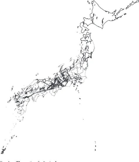
N Japan, we have so many earthquakes including smaller ones. On occasion of the 2011 Tohoku earthquake and the Great Hanshin earthquake, we had the great loss of human life in these disaster. The precise prediction of earthquakes has been expected for many years, but it is very difficult to include the estimations of locations and magnitudes. In the recent studies on the earthquakes, active faults are useful for estimating locations and magnitudes of earthquakes. Active faults are the discontinuity of strata which has the distortion of each rock plane. If the active fault breaks the stress, the accumulated geological energy will cause the earthquakes. In this article we investigate the distribution of active faults focusing on angles of faults devising the new test statistic with high performance even for small samples.The research on active faults and earthquakes has been studied for a long time. Especially the investigation into active faults and outbreak probabilistic model is also studied and discussed in Japan. We use the active fault database col-lected by National Institute of Advanced Industrial Science and Technology[1]. The table I shows the specifications of the active faults in Japan. We should explore the property of active faults for anti-disaster from the statistical view-point.
TABLE I
SPECIFICATIONS OF THE ACTIVE FAULTS INJAPAN
Number of faults named 559
Number of the sum of elements by segment 3069
Total length [km] 10803
II. TESTING FOR DIRECTIONAL UNIFORMITY
In the first place, we shall be aware of dangerousness of the active faults in the same directions, and we are interested in
Manuscript received July 23, 2015, revised July 28, 2015. This work was supported by JSPS KAKENHI Grant Number 26240003.
Y. Akimoto is with Graduate School of Science and Engineering, Chuo University, 1-13-27 Kasuga, Bunkyo-ku, Tokyo 1128551, Japan. e-mail: [email protected]
T. Sakumura is with Department of Science and Engineering, Chuo University, 1-13-27 Kasuga, Bunkyo-ku, Tokyo 1128551, Japan. e-mail: [email protected]
T. Kamakura is with Department of Science and Engineering, Chuo University, 1-13-27 Kasuga, Bunkyo-ku, Tokyo 1128551, Japan. e-mail: [email protected]
testing uniformity of the directions of faults against the uni-form directions. Mardia[2] described the Rayleigh test when mean direction is given based on von Mises distribution ([3], [4]), whose density function is expressed by the following:
f(θ;µ, κ) = 1 2πI0(κ)
exp(κcos(θ−µ)).
Whereκandµdiscribe the parameter of concentration and mean direction respectively. The score statistic is is obtained using the convenient parameter transformation,
ω= (κcosµ, κsinµ)T.
Uniformity is corresponding toκ= 0, and the transformation gives rise to ω = 0, which can give us very simple score statistics free from any evaluation of parameter estimation.
S1 = 2nR 2
.
Another test is a just variant of the above test statistic, which is also known as Rayleigh test or V-test ([5], [6], [7], [8], [2], [9], [10], [11], [12], [13]):
S2 =
2
n { n
∑
i=1
cos (µ−θi) }2
.
The parameterµincluded in the statisticS2is replaced by the specified directionθ0. In our study we replacedθ parameter by theoretical mean value of uniform distribution on(0,2π), E(θi) =π. In our experiencesS1statistic does not have good performance in that it does not assure that α-critical levels and high powers against alternatives (smallκ) especially for small samples. In this article we will propose the new test statistic based on the LM test and investigate the behavior of this statistic and apply this test to active faults data in Japan. The normal von Mises distribution is defined on(0,2π), but our directions of active faults must be the distribution defined on(0, π). We consider the following conditional distribution,
f(θi;µ, κ) =
1
2πI0(κ)exp(κcos(θi−µ))
∫ π
0 1 2πI0(κ)
exp(κcos(θ−µ))dθ . (1)
(0≤θ, µ < π, κ≥0)
Tedious calculations of likelihoods give us the following new test statistic:
S3 =
{
−2n
π sin ˆµ+ n ∑
i=1
cos (ˆµ−θi) }2
n
2 − 4n π2 sin
2µˆ
.
Fig. 1. The active faults in Japan
III. SMALL SAMPLE BEHAVIOR OF THE TEST STATISTICS
We study the small sample behavior of the test statistics based on the random segment spread on the two-dimensional space. The test statistic S3 is basically explain to the half angular space (0, π). For comparison of these statistics we generate the uniform random numbers on(0, π), and we use the 2×θi for S1 andS2 andθi for S3, because the former two statistics are ones designed for testing for the uniformity of(0,2π). In our study we need just test statistic defined on half circle (0, π). The Table II and Table III show that our proposed statistics conditioned on the half circle based on the conditional distribution has moderately good performance. We can say that the performance of the test statistics are as follows:
S1≺S3≈S2.
However, as we conventionally use the test statisticsS1and
S2 defined on full circle, and we must use theS3 from the conditioned distribution.
TABLE II
THE NOMINAL AND THE ACTUAL LEVELS OF SIGNIFICANCE(RANDOM SAMPLE SIZE OFnFROM THE CONDITIONAL VONMISES DISTRIBUTION
κ= 0)
n 1% 2.5% 5% 10%
3
proposed A 0.005 0.027 0.067 0.142 proposed B 0.000 0.001 0.016 0.141 proposed C 0.007 0.017 0.035 0.097 Rayleigh test 0.000 0.000 0.001 0.106 V-test 0.000 0.072 0.174 0.298
5
proposed A 0.015 0.035 0.067 0.128 proposed B 0.001 0.014 0.060 0.156 proposed C 0.007 0.020 0.046 0.100 Rayleigh test 0.001 0.016 0.043 0.095 V-test 0.028 0.076 0.144 0.274
10
proposed A 0.012 0.027 0.053 0.107 proposed B 0.008 0.028 0.065 0.135 proposed C 0.009 0.023 0.048 0.100 Rayleigh test 0.007 0.021 0.046 0.098 V-test 0.032 0.078 0.147 0.264
20
proposed A 0.009 0.024 0.049 0.099 proposed B 0.011 0.030 0.062 0.124 proposed C 0.009 0.024 0.049 0.100 Rayleigh test 0.008 0.023 0.048 0.099 V-test 0.034 0.079 0.146 0.261
50
proposed A 0.010 0.025 0.049 0.099 proposed B 0.011 0.029 0.058 0.113 proposed C 0.010 0.025 0.050 0.100 Rayleigh test 0.009 0.024 0.049 0.100 V-test 0.035 0.081 0.146 0.259
100
proposed A 0.010 0.025 0.050 0.100 proposed B 0.011 0.028 0.054 0.107 proposed C 0.010 0.025 0.050 0.100 Rayleigh test 0.010 0.025 0.050 0.100 V-test 0.036 0.081 0.147 0.259
Athe proposed statisticsS
3(the width of sample range for ˆ
µ).
Bthe proposed statisticsS
3(the sample mean forµˆ).
Cthe proposed statisticsS
3(the theoretical mean forµˆ).
TABLE III
THE POWERS OF THE TEST(RANDOM SAMPLE SIZE OFnFROM THE CONDITIONAL VONMISES DISTRIBUTIONκ= 1)
n 1% 2.5% 5% 10%
3
proposed A 0.008 0.123 0.234 0.366 proposed B 0.000 0.004 0.053 0.277 proposed C 0.012 0.029 0.054 0.114 Rayleigh test 0.000 0.000 0.001 0.194 V-test 0.000 0.139 0.292 0.441
5
proposed A 0.144 0.244 0.338 0.450 proposed B 0.008 0.069 0.208 0.380 proposed C 0.015 0.034 0.065 0.123 Rayleigh test 0.007 0.067 0.145 0.256 V-test 0.105 0.218 0.336 0.506
10
proposed A 0.249 0.344 0.433 0.537 proposed B 0.114 0.233 0.353 0.496 proposed C 0.021 0.045 0.080 0.142 Rayleigh test 0.100 0.196 0.303 0.442 V-test 0.249 0.397 0.532 0.676
20
proposed A 0.305 0.401 0.489 0.591 proposed B 0.310 0.453 0.571 0.689 proposed C 0.032 0.063 0.106 0.178 Rayleigh test 0.325 0.470 0.594 0.721 V-test 0.535 0.683 0.787 0.876
50
proposed A 0.343 0.447 0.540 0.644 proposed B 0.738 0.830 0.888 0.933 proposed C 0.068 0.121 0.186 0.281 Rayleigh test 0.858 0.923 0.957 0.980 V-test 0.943 0.974 0.988 0.995
100
proposed A 0.401 0.515 0.613 0.716 proposed B 0.966 0.983 0.991 0.996 proposed C 0.141 0.227 0.319 0.437 Rayleigh test 0.997 0.999 1.000 1.000 V-test 0.999 1.000 1.000 1.000
Athe proposed statisticsS
3(the width of sample range for ˆ
µ).
Bthe proposed statisticsS
3(the sample mean forµˆ).
Cthe proposed statisticsS
IV. THE APPLICATION TO ACTIVE FAULTS DATA
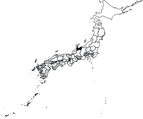
[image:3.595.45.293.184.390.2]As we mentioned in the previous section, the active faults in the same direction may be dangerous. We test the uniformity of direction of line segments approximating the faults by picking up both ends of observed faults. The Figure 2, Table IV and Table V show the q = 1−p-value. Thick color is corresponding to higher value of q. The high q -values indicates possibilities of non-uniformity of directions of faults.
Fig. 2. The non-uniformity of the active faults in Japan
TABLE IV
THEPREFECTURES WHOSEq-VALUE IS LARGER
Prefecture q-value Toyama 0.956
Osaka 0.836
Yamanashi 0.455 Fukuoka 0.359
Tokyo 0.351
TABLE V
THEPREFECTURES WHOSEq-VALUE IS SMALLER
Prefecture q-value Hokkaido <2e-16 Yamagata <2e-16 Akita <2e-16 Oita <2e-16 Nagasaki <2e-16
A. generalized test
In addition, we consider that directional data exist in the restricted range (c1, c2). We derived the former conditional distribution function in (2).
f(θi;µ, κ) =
1
πI0(κ)
exp(κcos(2θi−µ)) ∫ c2
c1
1
πI0(κ)exp(κcos(2θ−µ))dθ
.(2)
(c1≤θ, µ < c2, κ≥0)
Therefore, we get LM test statistic LM′ is (3).
LM′=
{∑n
i=1cos (µ−2θi)−
n[sin(µ−2c1)−sin(µ−2c2)]
2(c2−c1)
}2
n{sin[2(µ−2c1)]−sin[2(µ−2c2)]}−4c1+4c2
8(c2−c1)
−n{sin(µ−2c1)−sin(µ−2c2)}2
4(c2−c1)2
. (3)
V. CLUSTERING
In this section, we consider the problem on clustering line segments based on the angular data. Here we note that the angular data are obserbed just in (0, π), that is we cannot abtain the directions of the segments. Then, we must classify these data using the restricted method of k-means to a half circle. We propose the following method considering the measure of angular distanceθandα.
arg min
α1,α2,...,αK
n ∑
i=1 min
j [1−cos (2θi−2αj)]. (4)
Algorithm 1directional clustering Input:
K (number of clusters)
Θ ={θ1, θ2, . . . , θn} (directional data of line segment) Output:
A={α1, α2, . . . , αk}
l(i)|i= 1, . . . , n(cluster labels ofθi)
A← chooseK αj’s from angular data sample Θas the nodes randomly
repeat
Aprevious←A fori= 1tondo
l(i)←arg min
j
[1−cos (2θi−2αj)] end for
forj= 1tok do
A←mean.direction({θi} |l(i) =j)from (5) end for
[image:3.595.297.549.302.607.2]untilAprevious̸=A
Figure 3 shows the result of clustering Japanese active faults.
Fig. 3. The result of clustering Japan active faults
[image:4.595.54.279.561.763.2]Fig. 4. The result of clustering Fisher’s lineament data (proposed method)
Fig. 5. The result of clustering Fisher’s lineament data (normalk-means)
VI. DISCUSSIONS
We derived the LM test statistic for the conditional von Mises distribution which has relatively high performance even for small samples as the extension of V-test to half circle, we could find the areas of non-uniformity of active faults. We also proposed the new method of clustering technique for angular data. Further investigations will be needed considering locations and length of the active faults.
APPENDIXA
DERIVATION OFLMTEST STATISTIC
Likelihood function and Log likelihood function of the conditional von Mises distribution (1) is
L(θi;µ, κ) = n ∏
i=1
f(θi;µ, κ),
l =
n ∑
i=1
logf(θi;µ, κ)
=
n ∑
i=1
[κcos(θi−µ)−logI0(κ)−
log(2π)−logZ(µ, κ)],
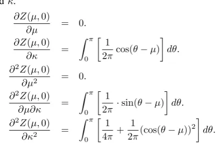
where I0 denotes the modified Bessel function of the first kind and order0, andZ(µ, κ)can be defined by
Z(µ, κ) =
∫ π
0 1 2πI0(κ)
exp(κcos(θ−µ))dθ.
andκ.
∂Z(µ,0)
∂µ = 0.
∂Z(µ,0)
∂κ =
∫ π
0
[
1
2πcos(θ−µ) ]
dθ.
∂2Z(µ,0)
∂µ2 = 0.
∂2Z(µ,0)
∂µ∂κ =
∫ π
0
[
1
2π·sin(θ−µ) ]
dθ.
∂2Z(µ,0)
∂κ2 =
∫ π
0
[
1 4π+
1
2π(cos(θ−µ))
2
] dθ.
Thus, substitute each partial differentiation for this result whereA(κ) =I1(κ)/I0(κ).
∂l ∂µ = n ∑ i=1 [
0·sin(θi−µ)−
1
Z(µ,0)
∂Z(µ,0)
∂µ ]
= 0. ∂l ∂κ = n ∑ i=1 [
cos(θi−µ)−A(0)−
1
Z(µ,0)
∂Z(µ,0)
∂κ ] = n ∑ i=1
[cos(θi−µ)]−
2n π sin(µ).
∂2l
∂µ2 =
n ∑
i=1
[−0·cos(θi−µ)
−
(
−1
Z2(µ,0)
(
∂Z(µ,0)
∂µ )2
+ 1
Z(µ,0)
∂2Z(µ,0)
∂µ2
)]
= 0. ∂2l
∂µ∂κ =
n ∑
i=1
[sin(θi−µ)
−
(
−1
Z2(µ,0)
∂Z(µ,0)
∂κ
∂Z(µ,0)
∂µ
+ 1
Z(µ,0)
∂2Z(µ,0)
∂µ∂κ )] = n ∑ i=1
[sin(θi−µ)]−
2n π cos(µ).
∂2l
∂κ2 =
n ∑
i=1
[
−A′(0)−
(
−1
Z2(µ,0)
(
∂Z(µ,0)
∂κ )2
+ 1
Z(µ,0)
∂2Z(µ,0)
∂κ2
)]
= 4n
π2sin
2(µ)−n 2.
Finally, calculate the score statistic by Lagrange multiplier using Hessian matrix. we call this statistic LM test statistic.
H =
[
H11 H12
H21 H22
] =−
∂2l
∂µ2
∂2l
∂µ∂κ ∂2l
∂µ∂κ ∂2l ∂κ2
.
J = [ d1 d2
] = [ ∂l ∂µ ∂l ∂κ ] .
LM = dT2(H22−H12t H− 1 11H21)−
1
d2.
S3 =
{
−2n
π sin ˆµ+ n ∑
i=1
cos (ˆµ−θi) }2
n
2 − 4n π2sin
2µˆ
a
∼χ21.
APPENDIXB DIRECTIONAL STATISTICS
In directional statistics, we cannot calculate arithmetic mean, then the mean direction θ is often used [9]. the mean direction is angle of resultant vector of observations. description of this in complex plane is (5),
θ = arg
n ∑ j=0
cosθj+i n ∑
j=0 sinθj
. (5)
Also,R that is the length of resultsnt vectorR is used for a measure of concentration of a data set.
R =
( n ∑
i=1 cosθi,
n ∑
i=1 sinθi
) .
R = ∥R∥
n .
RResultant vector
θ1
θ2
[image:5.595.57.281.61.205.2]θ3
Fig. 6. The resultant vector which indicated the mean direction
REFERENCES
[1] G. S. of Japan of National Institute of Advanced Industrial Science and T. (AIST), “Active fault database of Japan,” https://gbank.gsj.jp/ activefault/index e gmap.html.
[2] K. Mardia,Statistics of Directional Data, ser. Probability and Mathe-matical Statistics a Series of Monographs and Textbooks. Academic Press, 1972.
[3] S. Jammalamadaka and A. Sengupta,Topics in Circular Statistics, ser. Series on multivariate analysis. World Scientific, 2001.
[4] R. Von Mises, “ ¨Uber die“ganzzahligkeit”der atomgewichte und verwandte fragen,”Phys. z, vol. 19, pp. 490–500, 1918.
[5] E. Batschelet, Circular Statistics in Biology, ser. Mathematics in biology. Academic Press, 1981.
[6] J. Davis,Statistics and Data Analysis in Geology. Wiley, 2002. [7] D. Durand and J. A. Greenwood, “Random unit vectors ii: Usefulness
of gram-charlier and related series in approximating distributions,”The Annals of Mathematical Statistics, vol. 28, no. 4, pp. pp. 978–986, 1957.
[8] J. A. Greenwood and D. Durand, “The distribution of length and components of the sum ofnrandom unit vectors,”Ann. Math. Statist., vol. 26, no. 2, pp. 233–246, 06 1955.
[9] K. Mardia and P. Jupp, Directional Statistics, ser. Wiley Series in Probability and Statistics. Wiley, 2000.
[10] L. R. F.R.S., “Xii. on the resultant of a large number of vibrations of the same pitch and of arbitrary phase,”Philosophical Magazine Series 5, vol. 10, no. 60, pp. 73–78, 1880.
[12] M. A. Stephens, “Tests for randomness of directions against two circular alternatives,”Journal of the American Statistical Association, vol. 64, no. 325, pp. 280–289, 1969.
[13] S. M. Swan, A. R. H., “Introduction to geological data analysis,” International Journal of Rock Mechanics and Mining Sciences and Geomechanics Abstracts, vol. 32, no. 8, p. 387A, 1995.