Fault Localization in Distributed Adaptive Systems
by
Amit Raj, M-Tech.
Supervisor : Prof. Siobh´an Clarke
PhD Thesis
University of Dublin, Trinity College
Contents
List of Tables vi
List of Figures vii
Chapter 1 Introduction 1
1.1 Motivation . . . 1
1.2 Problem . . . 2
1.3 Challenges . . . 3
1.3.1 Inaccessible Faulty Components . . . 4
1.3.2 Inaccurate Diagnosable Information . . . 4
1.4 An Overview of Research . . . 6
1.5 Thesis Contribution . . . 9
1.6 Thesis Structure . . . 10
1.7 Chapter Summary . . . 11
Chapter 2 Related Work 13 2.1 Causal Graphs Models . . . 14
2.2 Bayesian Networks . . . 15
2.3 Program Slicing Techniques . . . 17
2.4 Ontology-based Models . . . 18
2.5 Structural and Statistical Equation Models . . . 20
2.6 Probabilistic Ranking . . . 21
2.7 Fault Localization in Practice . . . 25
Chapter 3 System Model and Fault Management Scope 31
3.1 Terminology and Scope . . . 31
3.1.1 Distributed Adaptive System . . . 32
3.1.2 Dynamic Adaptation . . . 32
3.1.3 Propagated Faults . . . 35
3.2 Problem Statement . . . 37
3.3 Existing Solutions . . . 40
3.3.1 Design-time Techniques . . . 40
3.3.2 Run-time Techniques . . . 42
3.4 Design Objectives . . . 45
3.5 Design Decisions . . . 48
3.5.1 Fault Localization in Adaptive Context . . . 48
3.5.2 System Monitor . . . 50
3.5.3 Knowledge-base . . . 52
3.5.4 Suspicious Components Isolation . . . 53
3.5.5 Faulty Candidates Localization . . . 55
3.5.6 Root Cause Analysis Integration . . . 58
3.5.7 Design Decisions Summary . . . 59
3.6 Chapter Summary . . . 60
Chapter 4 FaLDAS Fault Localization 62 4.1 System Execution . . . 63
4.1.1 Data Transformation . . . 64
4.1.2 Failed Execution . . . 65
4.2 Data Monitoring . . . 66
4.2.1 Data Monitoring Tool . . . 67
4.3 Fault Propagation Graph (FPG) . . . 70
4.3.1 FPG Model . . . 70
4.3.2 FPG Construction . . . 71
4.3.3 FPG Nodes Tagging . . . 73
4.3.4 FPG Analysis . . . 73
4.4 Fault Localization . . . 74
4.4.2 FaLDAS Ranking Algorithm . . . 75
4.4.3 FPGNode Health Determination . . . 78
4.4.4 FPGNodes Sorting . . . 78
4.5 Root Cause Analysis . . . 79
4.5.1 Existing Mechanisms . . . 79
4.5.2 FaLDAS RCA Integration . . . 80
4.6 Chapter Summary . . . 81
Chapter 5 Evaluation 83 5.1 Evaluation Parameters . . . 83
5.2 Related Algorithms . . . 84
5.3 System and Experimental Setup . . . 85
5.3.1 Experiments . . . 85
5.3.2 Data Generation . . . 86
5.4 Bootstrapping input data . . . 87
5.5 Time Efficiency . . . 88
5.5.1 Knowledge-base Construction . . . 89
5.5.2 Fault Localization . . . 93
5.5.3 Results . . . 94
5.5.4 Time Complexity . . . 95
5.5.5 Time Efficiency Significance . . . 95
5.6 Inaccessible Components . . . 96
5.6.1 Experiment . . . 97
5.6.2 Results . . . 102
5.7 Inaccurate Monitored Information . . . 103
5.7.1 Inaccurate Knowledge-bases . . . 104
5.7.2 Experiment . . . 108
5.7.3 Results . . . 108
5.8 Chapter Summary . . . 111
Chapter 6 Discussion and Future Work 113 6.1 Discussion . . . 113
6.1.2 Experiments Data Generation . . . 115
6.1.3 Fault Localization . . . 116
6.1.4 Multi-tenant Systems . . . 117
6.2 Future Work . . . 118
6.2.1 Inaccurate Information . . . 118
6.2.2 Accurate FPGNodes Isolation . . . 119
6.2.3 FPG Update . . . 119
6.2.4 Failure Classification . . . 121
6.2.5 Distinguish Propagated Faults . . . 121
6.2.6 Multiple Root Causes . . . 121
6.3 Chapter Summary . . . 122
Chapter 7 Conclusion 123
Appendix A Taint Analysis 126
Appendix B BARINEL Methodology 127
Appendix C Pinpoint Methodology 129
Appendix D Bayesian Belief Networks Methodology 131
List of Tables
2.1 The notations used in the computation of Similarity coefficient. . . 22
2.2 A sample hit spectra. . . 23
4.1 Hit Spectra of the sample system . . . 75
5.1 Experimental Setup . . . 86
5.2 Time efficiency significance in the context of adaptive systems . . . 96
5.3 TRANSFoRm System Faulty Candidates . . . 100
5.4 TRANSFoRm’s Hit Spectra . . . 102
5.5 TRANSFoRm pass/fail spectra . . . 102
5.6 Average Wasted effort for inaccurate input data . . . 109
6.1 Four cases related to input output values and faulty components . . . . 114
B.1 Probability of error for faulty candidate d2. . . 128
List of Figures
2.1 State of the art evaluation. . . 29
3.1 Example of component insertion adaptation pattern. . . 33
3.2 Example of component removal adaptation pattern. . . 34
3.3 Example of server reconfiguration adaptation pattern. . . 35
3.4 An example of propagated fault. . . 36
3.5 Problem description in a sample DAS before and after adaptation . . . 38
3.6 (a) Fault Propagation Map resulted from fault injection (b) Current system after adaptation. . . 41
3.7 Stack traces in the logs of components ‘C20’, ‘C7’ and ‘C21’ - After Adap-tation. . . 42
3.8 An excerpt of a Bayesian Belief Network for the sample DAS. The symbol p(X|Y) represents the posterior probability of hypothesis variable X for the evidence Y. . . 43
3.9 Example of incorrect BBN . . . 45
3.10 Example of inaccurate spectra . . . 46
3.11 Design Objectives to address the target system characteristics . . . 48
3.12 Overview of fault localization and root cause analysis in the context of adaptive system management. . . 49
3.13 Interceptor-based Monitoring Mechanism . . . 51
3.14 Description of the suspiciousness of a component in the context of dif-ferent output variables . . . 55
3.15 Process flow to identify and sort the faulty candidates. . . 55
3.17 An overview of design decisions to address the design objectives . . . . 59
4.1 An overview of the FaLDAS Fault Localization Approach . . . 63
4.2 An example system and execution . . . 63
4.3 State transformation of a sample system. . . 64
4.4 Description of Inaccessible Component . . . 67
4.5 Interceptor- and messaging bus-based software architecture . . . 68
4.6 An interceptor-based monitoring example with Apache Camel Messaging Infrastructure . . . 68
4.7 UML Metamodel of Components’ Run-time I/O values (IOV) . . . 69
4.8 Step by step execution of Algorithm 1. The left hand side represents an execution and the right hand side represents the corresponding FPG. . 72
4.9 Five executions of the sample system. . . 75
4.10 Three different traversed paths for three different execution along with their spectra. . . 77
4.11 Root Cause Analysis Flow . . . 80
4.12 Path-based root cause analysis. Image source: [69] . . . 81
5.1 Executions required to produce accurate results. . . 88
5.2 Data collection for FaLDAS . . . 90
5.3 Example of hit spectra construction from logs. . . 91
5.4 Example of pass/fail spectra construction from logs. . . 91
5.5 Example of BBN nodes and edges construction from logs. . . 92
5.6 Knowledge-base construction time. . . 92
5.7 Time Measurements of fault localization . . . 94
5.8 Overall time efficiency of approaches. . . 94
5.9 Example and effect of an inaccessible component. Component C1 is the actual faulty component but has inaccessible logs. (a) shows how FaL-DAS can access information even when component is inaccessible. (b) shows that other approaches are not able to access logs of an inaccessible component. (c) shows the FPG Spectra for FaLDAS. (d) shows spectra for BARINEL and Pinpoint with missing entry. . . 98
5.11 Wasted effort when actual faulty component is inaccessible in
TRANS-FoRm System. . . 103
5.12 Examples of FPG Spectra with correct and incorrect tags . . . 105
5.13 FPG Spectra representing the wrong tags of actual faulty node . . . 105
5.14 Inaccurate hit spectra. . . 106
5.15 Inaccurate pass/fail spectra. . . 107
5.16 Inaccurate BBN. . . 107
5.17 Wasted Effort analysis on simulated systems for inaccurate knowledge-base109 5.18 Wasted Effort analysis on TCAS systems for inaccurate knowledge-base 110 5.19 An example to show the impact of inaccurate information on fault lo-calization . . . 112
6.1 A component participating in more than one system. . . 118
6.2 An example of FPG with variable dependencies information . . . 120
6.3 An example of difference between FPGs before and after an adaptation 120 A.1 Taint Analysis: (a) Sample code for Taint analysis from [29], (b) Vari-ables composition . . . 126
B.1 BARINEL’s step by step execution. . . 127
C.1 Step by step exeuction of UPGMA [97]. . . 130
Abstract
Modern systems that execute in ubiquitous environments must be adaptive in or-der to maintain an acceptable quality of service. As in traditional distributed systems, faults in such systems are likely to propagate across several components and become manifest as apparently unrelated faults in components other than the responsible one. An efficient and accurate run-time root cause detection mechanism is required for fault recovery, which has been solved for non-adaptive systems. However, it is non-trivial in a distributed adaptive system (DAS) because of the changing nature of the system’s structure and behavior, the potential inaccessibility of adapted system components, and the potential for inaccurate diagnosable information about the system.
The key driver of this research is the observation about a debugging expert’s wasted effort in finding the root cause within a component where a fault’s symptom was ob-served. However, the root cause may exists in another component. The key idea is to pinpoint the actual faulty component. This thesis presents FaLDAS, a fault local-ization approach to find actual faulty components responsible to originate propagated faults in DAS. The contribution of the work are: (i) A novel fault propagation graph and its construction using components’ names and their run-time input/output values, (ii) Faulty Candidates’ detection which returns a sorted list of potentially faulty candi-dates, and (iii) A fine grained fault analysis which enables to find the potentially faulty corrupted variable, of a faulty component, whose propagation has caused a propagated fault.
run-time input output values enable the fault diagnosis of components whose internal designs e.g., source code, test cases, data flow, etc., are inaccessible. Unlike existing mechanisms which fail to diagnose inaccessible components, FaLDAS show substantial success in their diagnosis. In addition, detection of corrupted variable of a faulty com-ponent enables a debugging expert to find a specific root cause in a specific part of the component, which reduces root cause analysis effort.
FaLDAS’s fault localization algorithm finds a set of potentially faulty candidates. A candidate is a node in FPG (FPGNode) which has a reference to a potentially faulty component. In addition, FaLDAS sort the candidates according to their probability of being faulty. The final output of FaLDAS is the sorted list of candidates, which is a recommended order for a debugging expert to prioritize components for root cause analysis.
Chapter 1
Introduction
1.1
Motivation
Modern software systems play a crucial role in our daily life. Common systems in daily use are email, phone calls, traffic management, medical services, air traffic control, security, etc. Users are so dependent on software systems that any fault in such systems may result in loss of money and sometimes may cause death. For example, a technical malfunction in a Chinook helicopter ZD576 killed 29 people on board [108]. A software fault in computerized radiation therapy machine ‘Therac-25’ results in many deaths and serious injuries [75]. The Edwin I. Hatch nuclear power plant was forced into an emergency shutdown after a software update installed on a single computer [66]. Many software systems are so critical to our life that they must be robust, reliable and adaptive to automatically recover from a fault.
Faults in software systems are unavoidably introduced and to recover from a fault is costly. A NIST report estimates that software faults cost the U.S. economy $59.5 billion annually, approximately 0.6 percent of U.S. gross domestic product (GDP) [95]. A recent Cambridge University Research report states that the global cost of software faults has risen to $312 billion annually [44]. Moreover, this study found that approximately 50% of a software developer’s time is spent on finding and fixing faults. An efficient and accurate fault analysis and recovery mechanism is required to deliver a fault tolerant software system. Faults and their effects must be thoroughly analyzed and root cause analysis mechanisms must identify the faults efficiently and accurately.
1.2
Problem
Modern distributed systems are frequently composed of a range of components that collaborate in a potentially complex manner to achieve the overall systems’ goals. To maintain an acceptable quality of service for such systems in dynamic environments, individual components may be adapted i.e., upgraded, removed, replaced or reconfig-ured, at runtime, without interrupting the systems’ execution [102] [62]. For example, Popescu et al. [101] describe a crisis management system case study where differ-ent compondiffer-ents are imported to the system when the environmdiffer-ent or requiremdiffer-ents change. Such systems are referred to as Distributed Adaptive Systems (DAS). In a DAS, several components interact to provide a service, creating dependencies among the components. When a fault occurs, a dependency emerging through component interactions may cause the fault to propagate among inter-connected components [13]. Thus, the original fault becomes manifest as an apparently unrelated fault in compo-nents other than the responsible one [68] [70]. Such faults are referred to aspropagated faults (orexternal faults [13]). One of the important challenges in a DAS is to efficiently determine the root cause of a propagated fault.
further propagate to other components, say component B, which receives services from component A. The propagation of an fault from component to component is known as external propagation [13]. External propagation emerges in this example because the output of component A has deviated from correct output, causing incorrect input to component B, which results in a propagated fault to B. Propagated faults may further propagate to other components. In short, corrupted inputs and outputs between components cause fault propagation, and this thesis concentrates on supporting the identification of the root cause of such faults.
Beizer highlighted and analysed several different kinds of faults in a software sys-tem, in particular functional faults, structural faults, data faults (incorrect input and output), implementation faults, integration faults and architectural faults [16]. In this work’s occurrence frequency analysis, the frequency of data faults was estimated at 22.4%, the second most abundant in a software system. Also from Beizer’s analysis, a typical software program contains 50% lines of data declarations and assignments. Such program statements have the potential to become major sources of data faults, which in turn may cause propagated faults, and may severely impact the execution of a system. While the data fault frequency of 22.4% does not capture the majority of overall faults in a system, analysis of such faults is nonetheless potentially very time consuming, and is a substantial research field in its own right [41] [10] [8] [14].
1.3
Challenges
When a fault propagates and manifests as an unrelated fault in a component other than the responsible one, a two step fault diagnosis process is carried out as described below:
1. Fault Localization: The process for identifying the component responsible for gen-erating a fault [137] [132] [116] [110] [106].
2. Root Cause Analysis (RCA): The process for identifying the root cause of the fault within an identified faulty component [70] [69].
where the challenges presented by system adaptation are primarily manifest. Although Fault Localization is an extensively studied area, locating faulty components in a DAS remains challenging for reasons as follows:
1.3.1
Inaccessible Faulty Components
The diagnosis information needed about a component can be obtained by having: (i) ac-cess to the machine on which the component is hosted or (ii) acac-cess to the component’s diagnosable information such as logs or (iii) access to remote debugging capabilities for the component or (iv) access to the component’s source code or detailed internal design. When an adaptation imports components for which the DAS administrator (automated or not) has none of these access levels (i.e., the components are inaccessible), fault lo-calization is more challenging. In practice, such situations occur when Commercial Off-The-Shelf (COTS) components, Component Object Model (COM) components or any other blackbox components are included in a DAS. The designer has limited (or no) control that enables finding the information needed to analyze the root cause of a fault within the components [19]. Dependency analysis of such components is likely to be non-trivial [11]. Their failure semantics may be different from those of the other components in the system, so applying homogeneous failure analysis may not be suit-able [109]. Moreover, applying probes such as embedding a sensor or an agent inside such components may not be allowed.
1.3.2
Inaccurate Diagnosable Information
failure or success status of all 20 components is logged for a failed execution. In this case, a log has 20 lines, each with a <component name, success/fail indicator> pair for the execution under consideration. If any of the components either do not log success/failure at all, or log this incorrectly, then this will negatively impact the result.
Gap In Literature
To overcome such challenges in a DAS, the required input data must be dynamically generated and collected as existing data becomes inconsistent with the adapted system. In a DAS, obtaining a new configuration’s data at runtime is likely to be inefficient and the results may be incomplete or inaccurate. It has been observed that existing techniques use logs and error messages as preferred information to diagnose a fault [20] [17] [104]. Where logs are used to analyze faulty components, collective analysis of logs from multiple components, while possible, is non-trivial. This is because different logs may have different granularities, syntax and semantics [77]. Advanced logging techniques have been proposed to improve logging, but it remains difficult to correlate an error message with source code using logs [1] [139] [28]. For example, even knowing a component’s source code, a propagated fault’s error message “Exception in thread main: service endpoint not available” may not help to locate the actual faulty com-ponent and root cause within it. Developers also throw custom error messages which may be irrelevant or voluminous [77]. Moreover, a component’s log may not outline the execution context relevant to another component, as they may be loosely coupled and correlating different logs is a time consuming process. Overall, using logs is limited for faults’ correlation analysis and root cause determination.
1.4
An Overview of Research
A novel approach for fault localization has been designed to cope with the challenges of an adaptive system (Section 1.3). Based on valuable insights from existing ap-proaches, this thesis explores the possibility of constructing a knowledge-base about a system under consideration when the system exhibits the challenges described earlier. A heuristics statistical technique has been designed which reasons over the knowledge-base to locate the fault. The purpose of this approach is to provide an efficient fault localization useful for debugging experts to effectively identify the root cause of a prop-agated fault in a DAS.
Assumption This thesis makes the following assumptions about the environment in which debugging experts face challenges in analyzing the root cause of propagated faults.
1. The actual faulty component activates the fault within itself and cannot prevent it reaching the component’s interface. As a result the fault propagates, in the form of corrupted output data, to other components dependent on the actual faulty component. The other components receive corrupted input from the actual faulty component and may manifest it as a visible fault such as a system failure, outage, inconsistency, service unavailable, webpage not found, etc.
2. Components are loosely coupled in that they are independently developed and a component does not have information (internal structure and behaviour e.g., data flow, source code, test cases) about other components. They interact through well defined interfaces such as ESB communication bus.
3. The system’s operating environment is highly dynamic where components are frequently adapting (components’ addition and removal). An adaptive system re-configures itself at runtime in such a way that a number of components are added and deleted, and placed in a topology which cannot be foreseen at design-time.
the fault or its symptom appears. However, the debugging expert’s efforts are wasted when the fault’s root cause exists in another component. When the expert realizes that the root cause exists in another component, the expert finds the actual faulty compo-nent by analyzing other compocompo-nents and their diagnosable data. However, the actual faulty component may be inaccessible or the required information may be inaccurate or the system adapts so frequently that the expert has a limited time to analyze the fault. This means it is difficult for a debugging expert to efficiently identify the root cause of a propagated fault at runtime.
HypothesisThis thesis investigates how to identify the components actually respon-sible to originate a propagated fault. It frames its hypothesis as follows: The use of components’ real-time input output values enable to reduce the search space of finding the actual faulty candidate responsible for a propagated fault, to diagnose inaccessible components, and to identify actual faulty component even if its information in the knowledge-base is inaccurate.
the faulty components for a specific failed execution. This helps debugging experts to precisely identify the root causes for a particular failed run, efficiently. BARINEL’s output i.e., a set of faulty components, are not necessarily responsible for all failed ex-ecution. Different failed execution may have different sets of faulty components [112].
RequirementsA number of requirements analyzed for a fault localization mechanism to support the identification of an actual faulty component responsible for a DAS:
• Adaptation: The mechanism should be capable of identifying the fault in an adaptive system where components may adapt (add or remove) at runtime. Oth-erwise, an adaptation may occurs such that no faults traces, logs, or other ev-idences remains. Without evev-idences, fault analysis is difficult and the fault re-mains unresolved.
• Inaccessible Components: A mechanism should produce substantially correct results even if a DAS has several inaccessible components. A major impact of inaccessible components may be the inaccessibility of diagnosable information required for fault localization. As a result of inaccessible information, overall knowledge-base to reason about faults could be inaccurate or incomplete.
• Distributed Systems: A mechanism should work in a distributed system which may have several unknown components whose internal structure and behavior may be unknown, which impacts the fault localization. Otherwise, such compo-nents, which may be actually faulty one, remains undetected.
• Root Cause: In a DAS, a fault localization mechanism should be capable of identifying the actual root cause of a fault, i.e., faulty statements or corrupted variable responsible to cause a fault. Otherwise, fault recovery cannot be planned and applied. However, root cause analysis is not in thesis’s scope.
1.5
Thesis Contribution
This thesis investigates how an adaptive system’s run-time data can be used to effi-ciently identify the root cause of a propagated fault in a system. This research provides the following contributions to the knowledge:
Fault Propagation GraphExisting fault localization approaches generally use com-ponents’ runtime information, made available in logs. However, access to logs may be blocked in COTS components or time consuming to access and analyze. This the-sis describes a novel mechanism to construct a fault propagation model by analyzing only the real-time inputs and outputs of the components in the system. Even when the components are inaccessible, their requests and responses can be intercepted to read their inputs and outputs. This thesis describes an extension to directed acyclic graphs to represent an innovative fault propagation graph. An algorithm to construct a fault propagation graph from real-time inputs and outputs is presented, which has not been previously investigated. Generating the model in this manner supports ad-dressing adaptive system challenges and enables an efficient way to isolate suspicious components for a failed execution.
Faulty Candidates’ Detection Existing related mechanisms find a common set of faulty candidates as the root cause for multiple faults, which is not the optimal set of candidates responsible for individual faults [112]. This thesis describes an algorithm to efficiently isolate the faulty candidates responsible for a specific failed execution. The algorithm’s underlying statistical mechanism sorts the candidates according to their probability of being faulty. This algorithm innovatively finds the faulty candidates for a target failed execution, which has not been discussed by existing mechanisms.
faulty component along with its corrupted output variable. It helps a debugging expert to analyze only a part of the component, which has effected the computation of the corrupted output variable; likely to increase root cause analysis efficiency.
To compare the effectiveness of FaLDAS with that of other related approaches, a number of experiments carried out on simulated systems, TCAS [67] and TRANSFoRm [37] systems to investigate its diagnostic quality and time efficiency. The evaluation results show that FaLDAS achieves time efficiency up to two orders of magnitude while maintaining best diagnostic quality1 in finding inaccessible faulty component.
How-ever, FaLDAS does not performs best when information is inaccurate.
As a demonstration of how FaLDAS fits into an overall Root Cause Analysis process, FaLDAS is integrated with an existing RCA technique, which works with individual components in the ranked list. Le et al. [69] present an RCA mechanism which identifies the program statements responsible for corrupting an output variable. This mechanism was suitable to integrate with FaLDAS because FaLDAS identifies a faulty component along with its corrupted output variable, which might have propagated the fault. A debugging expert, using Le et al.’s approach, can identify the program statements, in the component, responsible for the corrupted output variable.
1.6
Thesis Structure
State of the art Chapter 2 analyses how existing mechanisms carry out run-time fault localization in adaptive system. In particular, the study explores the underlying data models and the reasoning algorithms used to find the faulty candidates. The chapter also identifies some mechanisms that can be applied to adaptive systems e.g., Spectra-based Fault Localization (SFL).
Design Chapter 3 discusses the basic terminologies used and describes the scope of this research. It then illustrates the problem statement with a detailed example and
analyses a number of existing mechanisms to solve the problem such as BARINEL [4] [2], Pinpoint [27] and Bellur et al.’s approach [17]. It then returns to the challenges of fault localization in adaptive system outlined in section 1.3 and describes the design objectives and design decision of this thesis which underlie the fundamental structure of the desired approach.
Approach Chapter 4 describes a detailed overview of the FaLDAS approach. It in-cludes the monitoring of an adaptive system, construction of a knowledge-base (i.e., fault propagation graph), a statistical mechanism and algorithm to localize the faulty components and finally ends with the description of FaLDAS’s integration with an existing root cause analysis mechanism.
Evaluation Chapter 6 evaluates FaLDAS’s time efficiency and diagnostic quality by comparing with that of other related approaches. It first describes the experimental set-up, in particular simulation-based system and the TCAS system. The time efficiency evaluation illustrates that FaLDAS achieves the significant gain (up to two orders of magnitude) over other approaches. However, the diagnostic quality evaluation illus-trates that FaLDAS achieves best accuracy to diagnose inaccessible components but not when information is inaccurate.
DiscussionChapter 7 summarizes FaLDAS and its achievements. It highlights a num-ber of scenarios where this research can be useful and not. A numnum-ber of limitations are discussed targeting the potential areas for future work.
1.7
Chapter Summary
effective fault localization mechanisms are required to analyze the faults.
A fault propagates among inter-connected components and becomes manifest as an apparently unrelated fault in components other than the responsible one. Analyz-ing the root cause of a propagated fault is a complicated problem. It becomes even more complicated in Distributed Adaptive System (DAS) where components adapt at runtime. Root cause analysis of a propagated fault is complicated in DAS because (i) inaccessible components may be adapted at runtime whose access to required informa-tion may be blocked, and (ii) the complicated and dynamic configurainforma-tion of a system limits the monitoring mechanisms to monitor accurate information of the system.
This thesis develops an approach to efficiently and effectively localize the faulty components responsible to originate a propagated fault. It presents a novel mechanism to construct a fault propagation graph using component’s real-time inputs and outputs. In addition, this thesis develops an algorithm which reasons the graph to analyze actual faulty component(s). The approach is evaluated for its diagnostic quality and time efficiency to compare with other related approaches. The results illustrate that the FaLDAS mechanism is two orders of magnitude efficient and achieves best quality to diagnose inaccessible faulty components.
Chapter 2
Related Work
Fault localization is an established field for non-adaptive systems, with considerable successes reported. A number of such techniques are included here, and while many of them were not designed for adaptive systems, both their capabilities in this regard are considered, and also the challenges they face even within non-adaptive systems. A number of more closely-related techniques for adaptive systems are also emerging, which have provided this thesis with useful insights.
Fault Localization approaches use a system’s data to construct fault propagation model which is analyzed to localize a fault. A Directed Acyclic Graph (DAG) is one of the popular techniques to represent the causal relationships between faults. Section 2.1 investigates approaches where a DAG is used to represent causal relationship between faults, dependencies between components, propagation of faults, etc., for fault localiza-tion. A variant of DAG i.e., Bayesian Belief Network (BBN) provides the probabilities of causality between software entities e.g., faults. Section 2.2 investigates BBN-based approaches which use probabilistic inferences to conclude the actual cause of a fault.
a component’s activities to conclude a list of potential faulty components. However, not all components in the list are actually faulty, they are sorted according to their probability of being faultiness. Section 2.6 analyzes such ranking mechanisms which sort the faulty candidates according to their faultiness for a failed execution. Lastly, section 2.7 presents existing fault analysis techniques currently used in the software industry.
2.1
Causal Graphs Models
A causal graph model represents the causal relationship between entities of a software system. This section analyzes graph-based fault localization techniques to localize faults in a DAS.
Candea et al. [21] describe an automatic failure-path generation technique that automatically generates fault propagation information of a system at design-time. They inject faults in one component and analyze their effects in other components. A fault is manually injected into a component. A monitoring mechanism detects the fault propagation across several other components. The system need to reboot for each fault injection and its propagation analysis. The mechanism does not require prior information about the components, but the process takes considerable time to run, and requires several reboots which is not possible in adaptive systems. Moreover, fault propagations analyzed at design-time becomes invalid after an adaptation as new component may be added and an existing one may have removed. In addition, it is difficult to inject faults into components at runtime, when the components are inaccessible, to manipulate the source code.
retrieving the faults from an inaccessible component is non-trivial. The identified rela-tionships between faults may be incorrect which results in incorrect fault localization. Moreover, in a DAS, such matrices would have to be re-generated after each adaptation, which becomes a performance bottleneck.
Yemini et al. [135] describe an event correlation technique in real-time. They consider a set of symptoms as a code that is decoded to analyze the problem. The technique uses the topology of the system to create a bipartite graph that is required to generate the code. In a DAS, the topology of the system changes, thus bipartite graph changes and hence the code is required to be regenerated. It limits its applicability in adaptive systems.
Le et al. [69] discuss a fault correlation technique based on the fault propagation paths. The premise of the approach is that when two faults occur in a single execution path, they are correlated. However, several faults are latent faults whose error or evidences do not appear or are difficult to detect. Where the root fault is a latent one, this mechanism is not likely to find the root fault and its root cause.
Several other graphical models exist to visualize large complicated systems. For example, Feng-wu et al. [131] describe a diagnostic tree, which effectively is an extended version of a fault tree, to analyze system-level faults. Another version of a DAG is Bond graphs in which arcs are bidirectional. These graphs are used to identify the bi-causality between two faults [83] [18]. These graphs, when compared to a DAG, provide more detailed information, particularly quantitative information. On the other hand, a DAG is mainly concerned with the qualitative characteristics of a system such as dependencies, fault propagations, data flow etc., which also can be easily visualized. Thus, a DAG is more widely used research and industry [133].
2.2
Bayesian Networks
A Bayesian Belief Network (BBN) is a probabilistic directed acyclic graph where nodes denote random variables and edges represent the conditional probabilities. It is a casual graph except that the nodes and edges support conclusions about the posterior probabilities. Let us assume a BBN where a nodef has a directed edge to nodeswhere
Bellur et al. [17] construct a BBN of faults. They use Jex tool [107] to discover and analyze a system’s call traces to generate components’ dependencies and to analyze fault occurrence evidences. Correspondingly, BBN nodes (<component, fault>) are constructed. Their assumption, if a component A uses component B then A’s exception E1 triggers B’s exception E2, is used to create edges between BBN nodes. However,
call traces, to construct BBN, are not always available for inaccessible components in a DAS. Motivated by this approach, FaLDAS constructed and used FPG where a node in FPG represents (<component, output variable>).
Joshi et al. [59] identify a fault using probabilistic inferences. At design-time, they determine a set of faults that can occur in a system. Such sets are characterized by a fault hypothesis e.g., a fault F occurrence corresponds to fault hypothesis ‘Server has crashed’ [59]. Bayesian probabilistic inferences are used to determine the responsible fault for each fault hypothesis. These pre-determined inferences are used to identify the actual cause of a system’s failure evidence i.e., a fault hypothesis, at runtime. However, such pre-determined probabilistic inferences are invalid after adaptation. Moreover, analyzing faults and their failures in an adapted systema priori is difficult as a DAS may adapt unknown or inaccessible components. Similarly, Lo et al. [82] create a Bayesian network where nodes represent components and edges represent the causal connection of components’ faults. When a fault evidence is detected, the Bayesian network inferences are used to locate the actual faulty component.
2.3
Program Slicing Techniques
Program slicing is a well known technique to analyze program statements, particularly in the field of fault localization [114] [73] [9] [74]. Program slicing divides a program into a group of statements responsible for a specific computation. These groups of statements are known as program slices. A software developer analyzes the data and control flow between slices to effectively pinpoint a slice which effects a program’s output, in particular a corrupted output value.
A number of specialized program slicing techniques exist such as static slicing, dynamic slicing, intra-procedural slicing, backward slicing, etc., [114]. A static program slice corresponding to a variable contains all the execution statements that may effect the variable’s value. The fault domain search is reduced to the slices which contain that variable [6]. Since, the program slices are constructed statically, they may not be the most optimal slices in a dynamic environment because the identified slices responsible for a corrupted variables may also include slices which should not be included [128]. Moreover, fault localization using static slicing is limited to the available test cases which may not cover all possible inputs to a DAS at runtime [128].
To construct an effective set of program slices, researchers have used an advanced technique with dynamic program slicing [73] [9] [74]. Lei et al. [74] present their approximate dynamic backward slicing technique which manages the trade-off between the size and accuracy of a slice to create an effective set of slices. The approach presents an algorithm that automatically analyzes the statements which directly or indirectly effects the output value of a variable. The set of slices is fed as input to their slice-based statistical fault localization tool which assigns different probabilities to slices based on their suspiciousness of being faulty.
Mariani et al. [84] produce code fixes for known problems, requiring the program’s bug-raising lines of code as input. This fault analysis approach is based on pass/fail tests, which needs a diverse set of test cases and a significant amount of execution time. However, obtaining the bug-raising lines of code is one of the biggest challenges for inaccessible components. Where the components are accessible, researchers have generated a knowledge-base of faults and apply expert systems for fault localization. Expert system approaches involve rule-based reasoning [35], model-based reasoning [85] or case-based reasoning [115]. These techniques work well for either small or static systems, though must be customized to a specific system. Also, a noisy or incorrect knowledge-base is likely to negatively impact the fault localization results.
In the program slicing literature, program slicing-based fault localization techniques generally depend on the test cases coverage [114] [73] [9] [74]. However, in a DAS that was composed dynamically at runtime, running test cases and obtaining their coverage is non-trivial. Another major problem with the program slicing techniques is access to the source code which may not be available for DAS components because several components may not be accessible, or if accessible, source code access may be blocked. Even if the source code of a components is accessible, the discussed mechanism do not specify how to use program slicing at the system level that includes several components. Moreover, in large-scale systems with a large code-base, there may be a large number of slices that need to be examined, which is not efficient [128].
2.4
Ontology-based Models
de-scribed in web resources. This information can be represented in a variety of formats. To describe an RDF document, RDFS (RDF Schema) presents an XML vocabulary to define RDF elements and relationship between those elements.
An ontology represents the fundamental objects and their relationships in a partic-ular domain. Objects are nouns and their relationships are verbs. For example, ‘bank has ATM’ represents ‘bank’ and ‘ATM’ as nouns and ‘has’ is a verb which represents the relationship between the two nouns. Web Ontology Language (OWL) is used to represent the formal semantics of an ontology. OWL is built upon RDFS objects. OWL is more powerful than XML in that it represents the semantics for encoding and ex-changing ontologies between different user groups, machines, languages etc. The OWL data model consists of several triplets having subject, predicate and object. A triplet is represented in XML syntax. A subject represents a particular resource of a domain which has a property denoted by predicate where object is the instance value of that property.
Zhou et al. [142] describe a fault propagation analysis in networked control sys-tems. Zhou et al. describe an approach to capture the entire structural and behavioral information of a system in ontology-based models. They describe two types of ontol-ogy of a system: centered ontolontol-ogy and system-centered ontolontol-ogy. The object-centered ontology represents the semantics of fundamental components of a system whereas system-centered ontology represents the semantics of the interactions between the components. When a fault occurs, fault and effect traces are used to reason about the ontology model. The outcome of such reasoning indicates the fault propagation paths. However, adaptive system challenges−inaccessible components and inaccurate information − restricts the construction of such ontology models in entirety. Inaccu-rate models negatively impact the outcome of the approach. Moreover, constructing ontologies after every adaptation is a time consuming and complicated process.
recovery action instead of finding the actual cause of the fault. The ontology of that component is sent across all the members so that a new member (added in place of a failed member) can understand this ontology and perform collaborative actions to tolerate the fault.
In ontology-based fault analysis, fault models are constructed using system ontology over which inferences are conducted. In such mechanisms, a system’s knowledge-base is represented in the form of an OWL ontology. Several tools exist to construct and store such ontologies such as protege, MediaWiki, etc. As these ontologies are constructed as an RDF data model, effectively in XML syntax, and queries can be formulated to conduct inferences. SPARQL, RDQL Versa and several other query languages exist to query an OWL ontology. SPARQL is one of the predominantly used languages and recommended by W3C.
In a DAS, a major challenge is the unavailability of the internal design of a compo-nent, and so constructing a detailed ontology of a component is non-trivial. Moreover, no ontology-based fault localization mechanism exist which works on real-time data. Most of the techniques work on structural information of a system and identify the structural faults.
2.5
Structural and Statistical Equation Models
Abreu et al.’s [4] mechanism is limited. Whereas FaLDAS can be used to find the faulty candidates for a specific failed execution. In addition, the evaluations shows that BARINEL is not as efficient as FaLDAS.
Similarly, in the Pinpoint algorithm, Chen et al. [27] create a program spectra which captures the failed or success status obtained from the logs of individual components, for a set of executions. Chen et al. track request/responses relating to individual components for a particular execution. They apply the Unweighted Pair-Group Method using Arithmetic Averages (UPGMA) algorithm on the spectra to identify the faulty components. This is likely to work for a DAS because diagnosable information is collected at runtime. However, the evaluations show it is computationally expensive and more in-efficient than FaLDAS.
Statistical equation models are also used to represent the causal relationship be-tween two variables. For example, equation z = x + y represents causal relationship of z with x and y. Baah et al. [14] present a probabilistic graphical model to rep-resent the causal relationship between the variables of a program. The probabilistic reasoning is used to rank the program statements identified as faulty. A limitation of such statistical techniques is that the program variables should be identified in advance to construct the hypothesis. However, where a DAS brings unknown and inaccessible components in the system, identification of such variables is not possible.
Such equation models require a detailed quantitative information about a system to effectively carry out Fault Localization. In a real-world large complicated system, it is a challenging task. It becomes more challenging when the system structure and behavior adapts at runtime. As discussed, other qualitative models exist such as directed graphs, dependency graph, topologies, etc., whose construction is easier as they represent high level qualitative information of a system.
2.6
Probabilistic Ranking
candidates with higher probability are analyzed prior to the ones with lower probability. To rank candidates, techniques generally use the concept of similarity (i.e., similarity coefficient) between a software entity behavior and error occurrences.
Similarity Coefficient
Fault localization techniques generally use systems information such as execution traces, logs, dependencies, etc. Such information e.g., execution traces, is used to identify the faulty candidates through analyzing the differences between correct execution informa-tion and failed execuinforma-tion informainforma-tion. A mechanism is required that can differentiate correct executions’s information from failed executions’s information. In other words, a mechanism is required to assess the similarity between two sets of information.
A statistical measure used to compare the similarity or diversity between two sets is called similarity coefficients. In data clustering area, similarity coefficient is measured on binary, nominally scaled data sets such as{0, 1, 0, 0} and {0, 1, 1,1}. Given any two such sets, a similarity coefficient calculates the overlap between the sets. To express the similarity, each combination of values in the two sets can be represented in four notations as described in Table 2.1.
Notation Set1 Set2
a11 1 1
a10 1 0
a01 0 1
[image:33.595.253.389.449.524.2]a00 0 0
Table 2.1: The notations used in the computation of Similarity coefficient.
The similarity coefficients are mostly used in spectrum-based fault localization tech-niques [138]. Several similarity coefficients exist out of which Jaccard [54] [27], Taran-tula [58] [112] and Ochiai [87] are most widely used in spectrum-based techniques [138]. A detailed description of these coefficients is given below (sj is the value of similarity
coefficient):
• Jaccard Coefficient: sj = a11+aa1101+a10
• Tarantula Coefficient: sj =
a11
a11+a01 a11
a11+a01+
a10
• Ochiai Coefficient: sj = √ a11
(a11+a01)∗(a11+a10)
As an example of how a similarity coefficient helps fault localization, a sample hit spectra is used [3] where ‘1’ and ‘0’ represents whether a software entity is used or not, respectively (Table 2.2). This spectra illustrates that software entity 4 is the mostly likely to be faulty because its information set has maximum similarity with the error set. In other words, a fault occurs only when software entity 4 was involved in the execution. The following section analyzes a number of spectrum-based fault localization techniques which rank the faulty candidates through a similarity coefficient.
Software Entities
input 0 1 2 3 4 5 error
S1 1 1 1 1 0 1 0
S2 1 1 1 1 1 1 1
Table 2.2: A sample hit spectra.
Ranking Faulty Candidates
Several static approaches use the pass/fail status of test cases to identify and rank faults [46] [130] [136] [4]. Existing techniques instrument a monitoring agent inside the code to obtain the runtime information about test suites [58] [79]. The instrumented monitor is responsible for tracking the executing entities such as suspicious program statements, suspicious components, inputs and outputs, pass/fail status of test cases, etc. The collected information is used in statistical techniques to compute the heuristic measure of suspicious entities. The heuristic measure indicates the probabilities of being responsible for test case failures. The suspicious entities are sorted according to their probabilities to indicate the level of likelihood for being faulty.
In addition, they performed experiments to evaluate its efficiency in which Tarantula was found six orders of magnitude faster than other techniques.
Abreu et al. [4] present an algorithm BARINEL and compared it with Tarantula. BARINEL is a fault localization algorithm that produces a sorted list of faulty can-didates. It takes the hit spectra [49] of a system as an input to the algorithm. The hit spectra captures the involvement of individual components in an execution through flags. The flag value ‘1’ and ‘0’ represents that the components was used and not used in an execution, respectively. An algorithm STACCATO [2], as a part of BARINEL, isolates the faulty components. The isolated components are further sorted according to components Bayesian probability of being faulty. Abreu et al. states that Bayesian probability is the foundation for the derivation of diagnostic candidates in any rea-soning approach. However, Bayesian probability calculation may become an NP-hard problem (Section 2.2).
Abreu et al. [4] found, in their experiments, that BARINEL outperforms the Taran-tula technique. BARINEL find 60% of the faults by examining less than 10% of the source code. With the same effort, the Tarantula technique finds only 46% of the faults. Moreover, in terms of effort required to identify the actual fault, BARINEL was found better than Tarantula. Overall, Abreu et al. concluded that BARINEL is an improvement over Tarantula approach for fault localization.
Gopinath et al. [45] illustrate a fault localization technique that includes spectra-based and specification-spectra-based analysis. It uses SAT technology to assess the satisfi-ability of correctness specifications to identify the faulty statements and to generate test cases for spectra-based fault localization. Correctness specifications are effectively first-order relational logic on the object of a program. Such specifications are written in the Alloy specification language [53]. In addition, it uses traces of a failed execu-tion to determine the list of statements which violated the correctness specificaexecu-tions. Such statements are further used in spectra-based localization to obtain their faultiness ranking.
is a contradiction to the reality of how large-scale software systems are developed. Moreover, constructing thorough test cases becomes more difficult in adaptive systems where the system’s structure and behavior is decided at runtime.
2.7
Fault Localization in Practice
The global software development community still see fault analysis as a significant challenge [38]. Organizations use customized fault analysis techniques sufficient to meet their current quality of service requirements. Still, failures effect their services’ availability. Fiondella et al. [38] report outage incidents for large companies such as Google, Rackspace, Microsoft, etc., where Rackspace has encountered 80, Google - 45 and Twitter - 33 outages. To prevent such outages, Naksinehaboon et al. [94] suggest rejuvenation of systems to improve availability. Many industrial practices mimic the whole system as a scaled-down version, to speed the faults analysis process. However, such scaled systems may not sufficiently exhibit the size and complexity properties of the original system [78].
Large companies, e.g., Google, have a significant dependency on the analysis of exe-cution traces in logs to identify faults in the servers [104] [105]. Where logs are used to analyze faulty components, collective analysis of logs from multiple components, while possible, is non-trivial. This is because different logs may have different granularities, syntax and semantics [77]. Advanced logging techniques have been proposed to improve logging, but it remains difficult to correlate an error message with source code using logs [1] [139] [28]. For example, even knowing a component’s source code, a propagated fault’s error message “Exception in thread main: java.lang.NullPointerException” may not help to locate the actual faulty component and root cause within it. Developers also throw custom error messages which may be irrelevant or voluminous [77]. More-over, a component’s log may not outline the execution context relevant to another component, as they may be loosely coupled and correlating different logs is a time consuming process. Overall, using logs is limited for faults’ correlation analysis and root cause determination.
components may be blocked and even if possible, the component structure may change while these processes are executing [88] [71]. Several mechanisms apply design-time techniques for Fault Localization in static systems [106] [116] [132] [110] [137], which could also be applied in a DAS where a new system configuration is known a priori [69] [21] [76]. However, it is not generally the case that all possible configurations of an adaptive system will be known at design time [111]. Nagappan et al. [93] use execution traces to create operational profiles for diagnostic tools. Nagappan et al. use regular expressions to extract log messages of interest. However, analyzing logs/traces in this manner requires an extensive set of regular expressions, which may not be feasible and may be difficult to maintain.
2.8
Summary
The Causal Graphs Models section investigates a number of causal graph-based fault localization techniques. Researchers have used graphs to analyze causal rela-tionships between several types of software entities. For example, a fault propagation graph represents causal relationship between faults, dependency graph represents data or control relationship between components, petri-nets were used to identify the data propagation, fault-testcase dependency matrix was used to analyze the faults that may caused test case failure. Another form of graph, i.e., Bond graph, was discussed to analyze the bi-directional relationship between faults. It was found that graphs are predominantly used in fault localization techniques because of its ability to represent the relationship between any type of entity. Moreover, it is simple and efficient in that several graph traversal techniques exist which are highly efficient. A system’s design e.g., fault propagations, dependencies between components, etc., can be represented in a graph and an offending entity can be identified through a graph traversal technique.
computa-tionally expensive and inference time may be exponential. In a DAS where system information is partially available, which is also a case with many real-world systems, several BBN nodes remain uninstantiated and BBN inferences become an NP-hard problem.
The Program Slicing Techniquessection investigates a number of program slicing techniques in the context of fault localization. These techniques divide a program’s statements into a group of statements corresponding to a variable, called slices. When a corrupted variable’s value cause an execution to fail, slices corresponding to the vari-able are identified as faulty. A major drawback to such technique is the requirement for access to source code, which may not be possible in a DAS because of inaccessible components. Moreover, the related literature indicates that such techniques generally work on test case coverage. However, running test cases at runtime in a dynamically assembled DAS is non-trivial. The number of program slices could be extremely large when a large-scale system has a large code-base. As a result, numerous slices need to be examined.
The Ontology-based Modelssection investigates a number of ontology-based tech-niques for fault localization. An ontology is the representation of the semantics of business terms and their relationships. OWL is an XML-based language to define the ontologies. Researchers have used detailed information about the structure and be-havior of systems to define ontologies. In addition, they use a reasoning engine which reasons over the corresponding ontology to analyze the fault for a given symptom. In dynamic environments where a system changes at runtime, the ontology needs to be regenerated, which is cumbersome and time-consuming. Moreover, it was found that where detailed information about a system is not available (of inaccessible com-ponents), the corresponding ontology is inaccurate and the reasoning engine produces incorrect results, i.e., the wrong root causes of faults.
about involved software entities. Obtaining such detailed data in a DAS is non-trivial because of the dynamically changing structure and behavior of the system. Moreover, in a large-scale system with large number of software entities, statistical techniques may be time consuming.
The Probabilistic Rankingsection describes the fault localization techniques where faulty candidates are sorted according to their probability of being faulty. Spectrum-based fault localization (SFL) is a popular technique (Section 2.6). It employs a statis-tical technique to which a number of inputs can be applied such as test case coverage, component;s involvement status, components failure/success status for a request, etc. Where SFL uses test case coverage, such techniques are impractical for a DAS as run-ning test cases in a dynamically assembled system is non-trivial. Moreover, a number of techniques indicate that they read the required input data from logs which could be extremely large for large-scale systems and impacts efficiency. To sort the candidates, probabilities are calculated based on the similarity of a component’s behavior to error occurrence behavior. The Ochiai similarity coefficient performs better than others such as Tarantula and Jaccard.
Fault Localization in Practicesection describes the current practices of fault local-ization in industry. Software developers rely on debugging the code through putting checkpoints in the source code and analyzing the variables’ real-time values at those checkpoints. Advanced logging and log analysis technologies are not generally used. Developers manually analyze the logs and call traces to find the root cause of a fault. Where components are distributed, developers communicate over emails or attend physical meetings to analyze the root cause of a fault.
carefully design FaLDAS and to compare with other existing approaches. The diagram highlights the following findings:
Figure 2.1: State of the art evaluation.
1. Existing techniques are inadequate to work when the components adapt at run-time. Techniques specify the collection of required information for fault localiza-tion assuming a static system. However, it is not menlocaliza-tioned that how to cope when such an information becomes invalid after an adaptation.
2. To the best of our knowledge, no mechanism exist that address the problem of inaccessible components. Existing mechanisms assume that the required infor-mation about all components is available, which is not the case in real-world systems. Existing fault localization mechanisms are effected when information is unavailable for actual faulty component.
invest a substantial amount of time in finding the actual root cause in a faulty component.
Chapter 3
System Model and Fault
Management Scope
This chapter introduces the basic terminologies, problem, and design objectives and decisions of FaLDAS outlined in this thesis. Firstly, it introduces the terminologies related to distributed adaptive systems, dynamic adaptation and faults in Section 3.1. Section 3.2 describes the problem with an illustrative example of a DAS. Section 3.3 assesses a number of existing solutions to solve the problem. Useful insights from existing techniques analysis guided the formulation of the design objectives (Section 3.4). This chapter ends with the description of the design decisions made to fulfill the design objectives (Section 3.5).
3.1
Terminology and Scope
3.1.1
Distributed Adaptive System
FaLDAS assumes a distributed, component-based system model, where components are subject to change at runtime, and faults may propagate across the system as a whole.
Definition 3.1.1. A Component is the building block of a DAS, and encapsulates a unit of functionality (either business or technical). A component is a unit of distribution and configuration, and can be independently developed and reused [65].
Definition 3.1.2. A Distributed Adaptive System (DAS) is a distributed system con-sisting of a set of interacting components, to which new components can be added, or any participant components can be deleted, or updated or their relationships with other components changed, at runtime. Any of these actions means that the DAS as a whole has been adapted.
A DAS may be composed of several software and hardware components such as a middleware, remote objects, databases, Java beans, application servers, etc. To maintain an acceptable quality of service, such components must be adapted. For example, a Tomcat application server is removed and IBM websphere is added or an existing Java bean is removed and a new Java bean is deployed in the software. The next section describes the considered adaptations, with examples.
3.1.2
Dynamic Adaptation
Component Insertion Adaptation Pattern
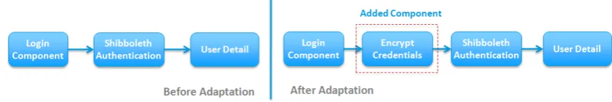
[image:44.595.96.537.312.386.2]The component insertion pattern describes the process of adding a new component into an existing target system [102]. An application of this pattern on a sample system is illustrated in Figure 3.1. This sample system is an access controller system on which a user enters their login details and the system authenticates the provided details using the Shibboleth authentication mechanism [90]. The system initially consists of three components: (i) A Login component which allows users to enter their login details, (ii) The Shibboleth Authentication component, which authenticates the login details, and (iii) A User Detail component which shows the logged in user’s details.
Figure 3.1: Example of component insertion adaptation pattern.
Component Removal Adaptation Pattern
[image:45.595.104.549.291.360.2]TheComponent removal pattern describes the process of removing a component from an existing target system. In real-world systems, an adaptation framework generally use state-based decision making to remove a component [43] [102]. To remove a compo-nent from a system, the framework checks if the compocompo-nent is inactive state, i.e., the component is doing a computation. When the component completes its computation, it is inpassive state. The adaptation framework performs the reconfiguration in which a passive state component is removed and dependencies are re-configured.
Figure 3.2: Example of component removal adaptation pattern.
As an example, let us re-consider the sample system where login details were trans-ported in encrypted form. The system is required to adapt to allow unencrypted data transportation between Login and Shibboleth components. The adaptation framework waits for these components to complete their current computations after which the Encrypt Credentials component is safely removed as shown in Figure 3.2.
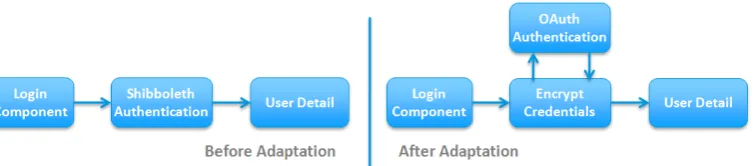
Server Reconfiguration Adaptation Pattern
The purpose of the server reconfiguration adaptation pattern is to add, remove and reconfigure the components. This adaptation pattern in turn is a combination of ponent insertion and component removal patterns [43] [102]. To reconfigure the com-ponents safely, the framework [42] wait for all the concerned comcom-ponents to complete their current computations and the new requests are redirect to a temporary buffer, to not loose them. The components are added, removed and reconfigured at runtime, and restarted to process requests.
dis-Figure 3.3: Example of server reconfiguration adaptation pattern.
cussed above. To the system reconfiguration adaptation pattern was applied which in turn applied insertion pattern to add ‘Encrypt Credentials’ and ‘OAuth Authentica-tion’ components, and applied removal pattern to remove ‘Shibboleth AuthenticaAuthentica-tion’ component. In addition, the dependencies among components are reconfigured as shown in Figure 3.3.
3.1.3
Propagated Faults
A fault is a system state where a required system constraint is violated [13]. Any system is likely to have vulnerabilities, which may activate and cause a fault such as buffer overflow, null pointer exception, etc. A fault prevents a component to produce the desirable output. The corrupted output in turn causes another fault in a different component dependent (directly or indirectly) on the actual faulty component. It causes a fault to propagate from one component to another component.
Definition 3.1.3. A propagated fault is a fault in a component where the root cause of the fault is in a different component. A propagated fault may have originated from one or many components, in which case it may have one or many root causes.
Definition 3.1.4. A faulty component is a component which has originated a gated fault. In particular, the component corrupted an output, which further propa-gates and causes a propagaed fault.
Definition 3.1.5. The root cause of a fault is the erroneous program statement(s) in the system where a system constraint was first violated, further causing faults in connected component(s).
[image:46.595.136.514.137.220.2]‘Shibboleth Credential’, which are responsible for taking user credentials as input, encrypting details and checking access, respectively. The dashed arrows from one com-ponent to another show the data flow between comcom-ponents. In ‘Login Comcom-ponent’, the variable ‘currentUser’ is set to ‘null’ which is sent to ‘Encrypt Credential’ com-ponent as a part of the request. ‘Encrypt Credential’ encrypts the user details and puts the encrypted data in variable ‘emap’ which is securely sent to ‘Shibboleth Au-thentication’ to assess user access. The user details are retrieved from the request and stored in variable ‘currentUser’. This variable is used to obtain the corresponding authentication code from an authentication store. However, this task encounters a fault ‘java.lang.NullPointerException’ because ‘currentUser’ is ‘null’ as shown in Figure 3.4. This fault is a propagated fault because its root cause is in the ‘Login Component’. The root cause is the ‘null’ assigned to ‘currentUser’ in ‘Login compo-nents’. In this case, ‘Login Component’ is the faulty component and statement ‘User currentUser = null’ is the root cause. The component ‘Encrypt Credential’ is not the faulty component because it does not modify the user details being transported, rather it just encrypt whatever it receives.
Figure 3.4: An example of propagated fault.
In the above discussed example, only one faulty component was responsible for originating the propagated fault. However, there may be situations where a propagated fault may have originated from one or many components, in which case it may have one or many root causes, respectively.
Definition 3.1.7. Multiple Components Faults. Where the vulnerabilities in more than one component causes the faults to propagate, resulting in a failed execution [27].
3.2
Problem Statement
Faults are inevitable in a system. This is partly due to increasing business pressure to release a software component to hard deadlines [92]. To achieve the deadlines, developers write a limited number of test cases, which may miss the testing of a number of potential faults. A component developed under such conditions is likely to cause a fault in a system. State-of-the-art fault localization techniques report a number of reasons for a fault (potential faulty components) and require substantial manual effort to correctly diagnose the actual faulty component and root cause within it [4].
Fault localization is even more complex because the root cause may not exist in the same component where the fault occurred. Fault activation while a system is running is likely to cause an error that may propagate and cause the failure of a service [13]. A component’s fault first causes an error within itself, which does not propagate to other interacting components until it leaves the boundary of the component. In fact, several faults may be handled within the component successfully. For example, the Java pro-gramming language provide constructs to catch Java exceptions in atry-catchblock. However, this is not always the case [57]. It is not always possible to provide a catch-ing mechanism for all possible faults in a system because of the system’s complicated structure and behavior [57]. Even if all exceptions are caught, it is unlikely that the component still produces the desired output. When a fault is not handled successfully within a component, the resulting errors propagate to the component’s interface. As a result, the service provided to other dependent components fails. The dependent components may receive corrupted input data that results in another fault unrelated to the original fault [13]. Effectively, a fault is propagated from one component to another component.
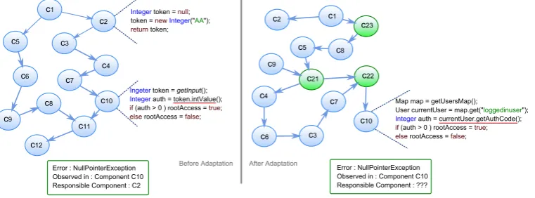
actual faulty component and potential root cause of a propagated fault in a DAS even when the DAS has inaccessible components or the system’s information is inaccurate. To explain the problem in detail, Figure 3.5 illustrates the problem using an example fault propagation in a sample DAS. Figure 3.5 shows an extended version of the sample DAS (discussed in Section 3.1.1) to introduce the complexities of a real-world system. This DAS is a distributed authentication framework that provides functionality to assess if a user is allowed root access to a secured resource. The example is motivated from real-world authentication systems such as Shibboleth [90] and OpenID [103], which provides federated authentication to several organizations such as the IEEE Institutional Login.
The left hand side of Figure 3.5 shows the sample DAS, before an adaptation, and is composed of a set of components (C1...C12). Two code snippets are illustrated: a fault
activates in co