Forecasting bus ridership with trip planner usage data : a machine learning application

(1)

Forecasting bus ridership with

trip planner usage data

a machine learning application

(2)

(3)

MSc thesis, March 2019 Program Industrial Engineering & Management Track Production & Logistics Management University of Twente

Author

Jop van Roosmalen

Supervisors:

dr. Chintan Amrit - University of Twente

dr. Engin Topan - University of Twente

dr. Niels van Oort - Delft University of Technology

Stephan Metz - OV-bureau Groningen Drenthe

Roy van den Berg - Translink

(4)

Management Summary

Public transport gives much attention to environmental impact, costs and traveler satisfaction. Good short-term demand forecasting models can help improve these performance indicators. It can help prevent denied boarding and overcrowding in buses by detecting insufficient capacity beforehand. It could be used to operate more economically by decreasing the frequency or the bus size if there is

overcapacity. It could help operators plan their buses during incidental occasions like big public events where little information is known and it can finally be used to reliably inform the travelers on the current crowdedness (Ohler et al., 2017; Van Oort et al., 2015a; Pereira et al., 2015).

This study investigates the usefulness of a new data source; the usage data of a trip planner for public transport. In the Netherlands there are multiple planners available to help find the most optimal (multimodal) travel advice. These trip planners require a date, a time, an origin and a destination, based on which they are able to construct multiple alternative journeys from which the user can choose. The usage data of these planners could potentially be very insightful, the main research question therefore is: Can one forecast short-term ridership of buses using data containing the consulted travel advices from a widely used trip planner for public transport and what accuracy can one achieve in different scenarios?

Literature

During the literature review no research was found using trip planner usage data for forecasting public transport demand. However, we found multiple factors which are interesting to include. We will include factors from the groups: Temporal, Demand characteristics, Weather, Event, Holidays and Transit characteristics.

Case study

For the study we used data of 20 lines (urban and regional) operated by Qbuzz in Groningen and Drenthe for the first three months of 2017. The time period is too short to investigate holidays and large public events.

Data

(5)

regression analysis is used to determine the forecasting potential of the trip planner usage data. This data is regressed towards smart card transaction data.

A few challenges had to be overcome in order to perform the study. Firstly, the data that is logged by 9292 is not optimized to be used for forecasting demand: It is unknown if two requests are made by the same person (viewing an alternative journey plan is logged as a separate request) and there is no identifier for the bus trip stored (only a line number). It is also difficult to match the trip planner trips with bus trips, since, over time, the 9292 private bus stops database evolved differently and there is no information stored on the actual delay although they are used during the construction of the travel advices.

Secondly, everyone has his own strategy (for different scenarios) in planning a trip and will use the planner differently to fulfill his needs. The user interface design and functionality of the trip planner influence this behavior and therefore directly impact the usage data. Furthermore, it is unknown if a travel plan is made for one person or for a group of people.

Methodology

We developed a model for forecasting the number of people boarding and a model for forecasting the number of people alighting at a certain stop. These forecasts are defined at the vehicle-stop level. By counting the number of people boarding and subtracting the number of people alighting along the trip, the forecasted number of passengers after a stop can be calculated (Ohler et al., 2017).

We compare five different machine learning models: multiple linear regression, decision tree, random forests, neural networks and support vector regression with a radial basis kernel (Zhang et al., 2017; James et al., 2013). We compare these models with two simple rules: 1 predict the same number as last week, and 2 predict the historic average as number. The models are implemented in the Scikit-Learn library of Python (Pedregosa et al., 2011) and the data is stored in a PostgresSQL database.

(6)

forests model. Finally, the hyperparameters of the models are tuned and the optimal configurations are stored. The scores are validated by using cross validation.

Results

We used the trips of one route during the morning peak to test our models. We used different kind of data partitions to train these models. All models are constructed with a planning horizon of 15 minutes. In most cases the best performing model used 20 features, the maximum number that was allowed.

The random forests model predicted the number of people boarding most accurate with a Root Mean Squared Error (RMSE) of 2.55 (R2 of 0.76). The random forests model forecasted the number of people alighting most accurate as well, with an RMSE of 2.20 (R2 of 0.76). The lower RMSE indicates that the number of people alighting is more predictable. In both cases the best version of the other models outperformed the forecasts of rule 1 and 2. It was discovered that subsampling had a slight negative effect.

When combining the boarding and alighting model, random forests outperforms the other machine learning models with an RMSE of 8.72. However, rule 2 has an RMSE of 8.603. When looking at the percentage of trips correctly forecasted within an absolute error of 5 passengers, rule 2 outperforms the random forests model with 84.08% against 58.9%. Thus, rule 2 outperforms the machine learning models when it comes to forecasting the number of passengers. Combining the best performing boarding and alighting model does not lead to the best forecast for the number of passengers. When looking at the percentage of correct maximum number of passengers predictions of trips – the most important indicator for adjusting the size of the bus –, the forecasts of rule 2 and the random forests model severely underestimated (more than 10 passengers lower as the real value) the maximum number of passengers for more than 27% of the trips.

(7)

Conclusion and recommendation

The trip planner usage data is an interesting source to detect the number of

additional people boarding or alighting. Especially since this process could be fully automated. However, the different organizations should adjust their data structures in order to construct more useful features, do more valuable analysis and to streamline the whole data preprocessing process of merging the different datasets.

(8)

Preface

This master thesis is the final stage of my master studies Industrial Engineering & Management with specialization Production and Logistics Management. It marks the end of my studies at two different universities.

I would like to thank Niels, Roy, Susan and Stephan who initiated the project and who gave me the opportunity to execute it. Furthermore, I would like to thank them, as well as Chintan and Engin, for their involvement, enthusiasm and

feedback without which this project would not have been possible. I also want to thank all the people at OV-bureau Groningen Drenthe for a welcoming working environment.

(9)

Table of figures

Figure 2.1: Framework of factors affecting transit use. ... 14

Figure 3.1 Left: Number of habitants per postcode-4; right: the postcode-4 areas with over 5000 habitants ... 17

Figure 3.2 Rate of habitants per urbanization category in the Netherlands and the provinces Groningen and Drenthe ... 18

Figure 3.3: Network map of the train, Qliner and Q-link. ... 20

Figure 3.4 The bus schedule for 2017. ... 22

Figure 4.1: The information streams between the different datasets. ... 25

Figure 4.2 Histogram of the recorded punctuality distribution for all recorded stop passages. ... 31

Figure 4.3 Distribution of the recorded delay aggregated over hours ... 31

Figure 4.4: Visualization for the different variants of line g554. ... 32

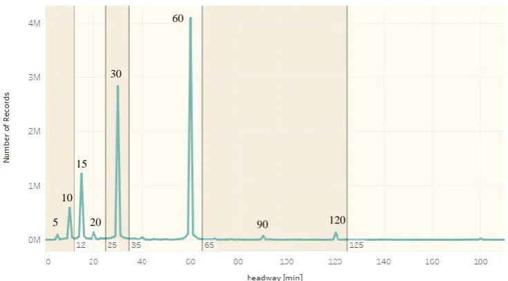
Figure 4.5: The distribution of the headway. ... 33

Figure 4.6 Homescreen of the webbased trip planner of 9292 with the trip planner magnified... 35

Figure 4.7 Travel suggestions in the web-based version of the 9292-trip planner. . 36

Figure 4.8: Difference between a journey question and its journey parts. ... 38

Figure 4.9 Requests per request interval ... 41

Figure 4.10 Number of requests aggregated over minutes after the hour ... 43

Figure 4.11 Number of departures aggregated over minutes after the hour ... 43

Figure 4.12: Flow of the smart card transaction data. ... 45

Figure 4.13: The number of check ins per date ... 51

Figure 4.14: The distribution of the frequency the smart card is used for a(n unchained) trip with Qbuzz ... 51

Figure 4.15: The distribution of the frequency the smart card is used for a similar trip ... 52

Figure 4.16: The 8 used weather stations and their id with the weights for bus stop Groningen Hoofdstation ... 53

Figure 4.17: A sample of the rainfall and duration of the rainfall per hour for 2 weather stations. ... 54

Figure 4.18: The distribution of the rain duration. The rain duration is stored per 6 minutes. ... 54

Figure 4.19: The 6 dimensional problem of matching the request to an actual bus trip ... 56

(13)

Figure 4.21: Grouping requests based on request interval. ... 58

Figure 4.22: Number of trips matched versus the allowed difference between start and end time for method 1 and method 2. ... 61

Figure 4.23: Departure time overlap according to the matched 9292 trips versus the sum of the absolute time differences ... 62

Figure 4.24: The number of transaction matched relative to the maximum summed absolute difference between departure time and check in time and arrival time and check out time ... 64

Figure 4.25: The relative trip frequency starting in a given hour. ... 66

Figure 4.26: The number of requests per check in or check out on weekdays ... 67

Figure 4.27: The number of requests per check in or check out on Saturdays ... 67

Figure 5.1: An example for the derivation of the number of passengers onboard from the forecasts of the two models. ... 74

Figure 5.2: The influencers of the forecasting performance ... 75

Figure 5.3: The line configuration g554-1-0 from Roden to Beijum with the corresponding stops ... 78

Figure 5.4: A distance-time diagram for the bus trips of data partition 1 ... 78

Figure 5.5: Cross validation set up ... 84

Figure 6.1: Feature importance of the boarding model for the line variant g554-1-0 and during a workday ... 93

Figure 6.2: Feature importance of the alighting model for the line variant g554-1-0 and during a workday ... 94

Figure 6.3: The RMSE of predicting the number of people boarding for trips of line variant g554-1-0 around 8 AM ... 96

Figure 6.4: The RMSE and the R2_{for the prediction of number of people boarding} ... 98

Figure 6.5: The RMSE and the R2_{for the prediction of number of people alighting} ... 102

Figure 6.6: The RMSE for predicting the number of passengers for g554-1-0 trips during morning peak ... 104

Figure 6.7: The predictions for the number of people onboard versus the real number ... 105

(14)

1

Introduc

(15)

1 Introduction

1.1 Research motivation

One of the main challenges in public transport is matching transport demand and supply given budget constraints. A mismatch in demand and supply leads to extended travel times, delays and less comfort in the short-term, which can have effect on the mode choice in the long-term. Ohler, Krempels and Möbus (2017) and Oort et al. (2015a) present multiple reasons why good demand forecasting is important. For instance, forecasts can be used to allocate buses to prevent

cramming in buses which results in more favorable travel conditions for travelers. By allocating buses where needed, no capacity will be wasted. Furthermore, this will prevent delays which are caused by extended alighting and boarding times during peak demands. Moreover, in the current high-tech era, travelers expect advanced accurate traffic information about expected arrival and departure times.

The fact that demand is fluctuating short term and long term, makes planning for sufficient capacity a complex task. For example, since travelers have different habits and activities over space and time, their need for public transport varies and is temporal and spatial dependent. Transit operators try to cope with fluctuations in demand by updating their network and timetable design one or two times a year. These reparations to the bus schedule involve high costs because of a snowball effect upon changes to underlying operations. During the year, some reinforcement buses are available at all time to be assigned if needed. However, insufficient supply is often detected too late. Sometimes this results in measures taken by traffic control, for example by sending (additional) buses. If insufficient supply could be forecasted, efficient matches in demand and supply could be realized. This can also avoid inconvenience for travelers.

(16)

effectively while delivering a higher quality of services. Big data can help to solve these contradicting requirements (Van Oort et al., 2015a; Van Oort et al., 2015b).

A big data source that could be interesting for forecasting public transport demand is the usage data of trip planners for public transport. Public transport trip planners are electronic tools where travelers can request a travel plan for a given time and date and origin and destination. The usage data consists of these user requests in combination with the travel plans which are consulted by the user.

Previous research into trip planners (e.g. Brakewood & Watkins, 2018) shows that trip planners reduce the (perceived) waiting time of their users, reduce the (perceived) travel time of their users and increase the public transport demand. Brakewood & Watkins (2018) also show that these kinds of real time travel information systems influence different choices like travel, mode, route, boarding stop and departure time. We did not find research focused on forecasting ridership with trip planner usage data. However, trip planner usage data could provide valuable information on the (short-term) transport demand.

This explorative research investigates the predictability of ridership of public transport by using trip planner usage data. The log data of the trip planner are fused with the transaction data of smart cards to investigate the correlation between consulted trips and trips made.

We will utilize a case study for this research. The case study consists of the bus network in Groningen and Drenthe. The network is planned and scheduled by OV-bureau Groningen Drenthe and operated by Qbuzz. For this study the data of 9292 was used. 9292 is one of the major trip planners in the Netherlands and includes all public transport modes for the whole country. The 9292 data is fused with the transaction data of the OV-chipkaart, the Dutch smart card valid for all public transport modes across the country. This transaction data represents the realized demand.

(17)

transport as a whole. For instance, there was an unexpected peak in passenger after the spring break in 2018 on lines with schools, which resulted in denied boarding and an article in the regional newspaper with the heading "Buses still on holidays, but pupils and students not" (Trimbach, 2018). In this case, OV-bureau was misinformed by one of the schools, but still held all the blame.

A second possible application of the new prediction method could be the planning of buses during large public events. Large public events or multiple smaller ones cause high variance in transport demand. As information on most events is limited and not centralized, their influence on the system is hard to predict (Pereira et al., 2015). The demand varies with the attractiveness of the event, the weather, whether the event is at night and whether people have to work the next morning. These buses are scheduled by OV-bureau based on trial and error and historical data. OV-bureau hopes to identify shortcoming supply before it happens and thus preventing inconvenience to passengers by forecasting the ridership. Unfortunately, the time period of the provided datasets does not include large events. Therefore, we cannot analyze the predictability of the demand in the scenario of a large event.

A third application is assigning the bus type dynamically. Changing to a smaller bus size could decrease the costs but also the carbon footprint.

Finally, the forecasts could be used to give more reliable information on the crowdedness in the bus. For instance, via the trip planner of 9292.

1.2 Research objective

The objective of this exploratory research is to determine whether usage data of a major trip planner can be used to predict the ridership of bus trips. There should be a correlation if the trip planner in question is widely used among the public

transport user: If there are more travel advices consulted for a particular hour, it is likely there are more travelers intending to use public transport during that hour. However, for the forecast to be valuable to the transit operator, this correlation should have a certain accuracy for time and space. More specifically, the operator should be able to predict the ridership for a certain bus trip. Otherwise, the log data of a trip planner are not an effective new information source for forecasting shortcomings in bus transportation supply.

1.3 Research questions

(18)

Can one forecast short-term ridership of buses using data containing the consulted travel advices from a widely used trip planner for public transport and what accuracy can one achieve in different scenarios?

By answering the following questions, the main research question will be answered.

1. What internal and external factors cause fluctuations in bus transport demand according to literature?

This question helps to get a better understanding about varying public transport demand. Transport demand varies with time and space. But other internal factors like fares and the type of buses can also influence the demand. The result of this question is a list of factors which influences the transit demand in Groningen and Drenthe per bus line.

2. What are the opportunities and challenges of using log data from the

9292-trip planner for forecasting ridership?

9292 is one of the major trip planners in the Netherlands and includes all public transport modes for the whole country. 9292 has designed algorithms to construct travel advices and a platform to communicate these advices with travelers. These designs effect which trips the traveler gets to choose from, which in turn effect the log data. This question investigates the consequences of selecting the log data of 9292 instead of other available trip planners. Furthermore, a list of requirements for trip planner data is derived.

3. What are the opportunities and challenges of using OV-chipkaart

transaction data to represent ridership?

The OV-chipkaart is the Dutch smart card valid for all public transport modes across the country. Travelers use the OV-chipkaart by tapping in and tapping out at the start and end of their journey and each time they change between operators or vehicles (except for trains and metros). However, this dataset is not all encompassing; there are still some other fare paying methods available. Therefore, it might be that some extra attention is needed when using data from a smart card. By answering this question, we create a better understanding on how to use the transaction data to represent ridership. We will also create a list of requirements for the smart card transaction data.

(19)

By answering the last research question, we get a better understanding of the relation between 9292 and the ridership. With this understanding we can answer the main research question.

1.4 Outline

The remaining chapters in this report are as follows: In chapter 2 the literature will be reviewed to answer the question: Which scenarios cause fluctuations in bus

transport demand in Groningen and Drenthe? Chapter 3 will discuss the used case

study in three parts. In the fourth chapter the different data sources and used datasets will be introduced. The fifth chapter explains the used methodology. Chapter 6 will introduce the results. The discussion of these results can be found in chapter 7. The final chapter includes the conclusion to the research questions and implications and recommendations for practice and science.

(20)

2

Literature revie

(21)

2 Literature review

A literature review is conducted to answer research question 1: What internal and external factors cause fluctuations in bus transport demand according to literature? Internal factors are factors that can be regulated by the transit operator, like fare and frequency. External factors are all other factors.

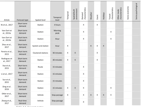
The literature search is conducted as recommended by Webster & Watson (2002). The exact used methodology can be found in Appendix B. The found literature is presented in the concept matrix shown in Table 2.1. The concept matrix shows the forecast type, aggregation level and concepts (types of used factors) extracted from the respective article. A concept is only attributed to an article if the article actively included the concept.

Article Forecast type Spatial level

Temporal

level Tem

p o ra l Sp at ia l/ b u ilt en vi ro n m en t D em an d ch ar ac teri st ic s W ea th er Ev en t Ho lid ay s Tr an si t ch ar ac teri st ic s O th er m o d e ch ar ac teri st ic s So ci o -ec o n o m ic So ci o -p sy ch o lo gi ca l

De Palma and

Rochat, 1999 Survey - - X X

Khattak and De Palma,

1997

Survey - - X X

Chakrabarti,

2016 Mode choice - - X X X

Hensher and

Rose, 2016 Mode choice - - X X X

Spears et al., 2013

Long term

demand - - X X X

Upchurch and Kuby, 2014

Long term

demand Station

Average

weekday X X X

Brakewood et al., 2015

Long term

demand Route

Average

weekday X X X X X

Kuby et al.,

2004 Long term Station

Average

weekday X X X X

Stopher, 1992 Long term

demand Route

Average

time period X X X X

Choi et al., 2012

Long term demand

Station to station (OD pair)

Average

time period X X X

Doi and Allen, 1986

Medium term

demand Route Month X X X

Tsai et al., 2009

Medium term

demand Station Month X X

Kalkstein et al., 2009

Short term

demand System Day X

Guo et al., 2007

Short term

demand System Day X X

Li et al., 2014 Short term

demand Average route Average day X X X X

Jiang et al., 2014

Short term

(22)

Article Forecast type Spatial level

Temporal

level Tem

p o ra l Sp at ia l/ b u ilt en vi ro n m en t D em an d ch ar ac teri st ic s W ea th er Ev en t Ho lid ay s Tr an si t ch ar ac teri st ic s O th er m o d e ch ar ac teri st ic s So ci o -ec o n o m ic So ci o -p sy ch o lo gi ca l

Ni et al., 2017 Short term

demand Station 4 hours X X

Van Oort et al., 2015a

Short term

demand Station

Morning

peak X X

Van Oort et al., 2015b

Short term

demand Station Hour X X

Zhou et al., 2017

Short term

demand System and station Hour X X X X

Pereira et al., 2015

Short term

demand Clustered stations 30 minutes X X X

Rodrigues et al., 2017

Short term

demand Station 30 minutes X X X

Xue et al., 2015

Short term

demand Route 15 minutes X

Li et al., 2017 Short term

demand Station 15 minutes X

Sun et al., 2015

Short term

demand Station 15 minutes X

Ding et al. 2016

Short term

demand Station 15 minutes X X X X

Ohler et al., 2017

Short term

demand Vehicle Stop passage X X X X X X

Zhang et al., 2017

Real-time demand

Vehicle Stop passage

[image:22.595.31.505.68.428.2]

X

Table 2.1: Concept matrix

Existing researched transit demand forecasting models can be categorized based on the length of the prediction horizon. Long-term models - with a prediction horizon of a year - are mainly used to help decide on capital-intensive transit-oriented investments and to investigate the impact of major changes in service and environment. Short-term models – with a prediction horizon of days or hours - can be used by public transport operators to increase/decrease supply (dynamic traffic management) and to timely notify travelers on possible crowding (Pereira et al., 2015). Most models focus on predicting regular demand (Li et al., 2017). Beside the development of demand forecasting models, surveys are used to investigate the stated preference of travelers regarding varying factors (Khattak and De Palma, 1997; De Palma and Rochat, 1999) and to develop mode choice models

(Chakrabarti, 2016; Hensher and Rose, 2016).

(23)

vary from system wide to vehicle-stop passage level. Temporal levels vary from month to single stop passages.

There is a consensus in research in the influence of time and date. Research shows effects of seasonality, type of day and time of day. Xue et al. (2015) observe that the AM peak is sharper than the PM peak since schools and jobs start at the same time but end at different times. Some researchers cope with these fluctuations in demand by calibrating a model per time period. For instance, Stopher (1992), calibrated a separate model for peak (combination on AM and PM peak), day and night for weekdays and Li et al. (2014) developed a model per season. Others tried to forecast the impact of time by including dummy variables for type of day and time period (Ohler et al., 2017). Tsai et al. (2009) coped with seasonality in the data by using a moving average. Some tried to cope with these fluctuations by converting the variables to relative ones. For instance, Zhou et al. (2017) utilizes the ridership for a given hour and weekday compared to the monthly average for that hour and weekday. This way the intraday trends and patterns in ridership are accounted for.

Spatial features (synonym for attributes or variables) are also considered important. In some articles this feature is avoided. For example, by only forecasting the ridership on route-level for one route. Other models use spatial features like built environment to denote the attractiveness of a stop or route for travelers. For instance, Kuby et al. (2004) included variables indicating the

intermodal connectivity of a station, such as accessibility, connecting services, park spaces, neighboring airports, type of station and variables as population and

employment within walking distance.

Another used explanatory variable for ridership is historic demand. Xue et al. (2015) used lagged demand with a week, day and 15 minutes interval to forecast ridership. Li et al. (2017) also uses lagged demand augmented by lagged demand of 18 other major stations in the system to predict the number of passengers alighting major metro stations in Beijing during special events. Ding et al. (2016) uses passenger counts of nearby bus feeder services to predict short term ridership for the metro. Van Oort et al. (2015a) and Van Oort et al. (2015b) used historic demand to represent the demand in the base scenario.

(24)

destination. It is possible that the people that change from public transport to private mode to avoid long walking in bad weather cancel out the people that go from private to public transport to avoid congestion. Furthermore, Kalkstein et al. (2009) conclude that the effect of seasons is little. Ridership is more dependent upon relative weather conditions. A travel survey conducted by De Palma and Rochat (1999) in Geneva shows that around 40% of the commuters are influenced by adverse weather conditions in their travel choices. They report that departure time choice was more affected as mode and route choice. These results are similar to the travel survey conducted by Khattak and de Palma (1997) in Brussels. Li et al. (2014) observed a negative influence of humidity, wind speed, rainfall and temperature on bus ridership in a region in Shanghai. They used absolute values of the weather variables but note that this approach may introduce influences not solely based on weather but also on seasonality due to the presence of a weather pattern throughout the year. Guo et al. (2007) utilizes relative weather variables for this reason. In their research they also noted that the weather-ridership relationship is more complex because it is based on how individuals perceive and prepare for the weather, the presence of a lagged effect and because some weather variables correlate while others are synergetic. Li et al. (2014) also observe that there is no consensus on the specific influence of weather variables. For instance, some studies showed a positive correlation between temperature and ridership whereas other studies showed the opposite. As stated in their paper, it could be that some study areas have a higher active mode share than others, resulting in a modal shift to walking and cycling when the temperature rises. Beside the direct influence of weather on travelers, it also has an indirect influence on the journey. For instance, adverse weather lengthens running times, dwell times and disrupts service

reliability (Guo et al., 2007).

Research agrees that events cause additional ridership. Kalkstein et al. (2009) stated that during events and festivals the ridership significantly changes. Rodrigues et al. (2017) tried to model this change utilizing information from the internet obtained via scraping and APIs on events to forecast the additional demand. Pareira et al. (2015) also scraped the information from the internet. They researched if the impact of an event could be predicted by including event

(25)

of events and holidays and therefore select a timespan in which they don't occur (Zhou et al., 2017).

Holidays also impacts ridership. Doi and Allen (1986) observe less demand during the summer holiday. Ohler et al. (2017) included three different type of holidays: public holidays, school holidays and semester breaks of the local

university. They researched two versions of representing these factors: via a binary dummy variable and via four dummy variables (days since the start, days left, days until next and days since previous). They propose the latter more elaborate way since they observe that demand also shifts just before and after a holiday. This demand shift was also observed by Kalkstein et al. (2009). To avoid these influences, they discarded these days from the dataset.

The characteristics of the public transport system also impact the ridership. Van Hagen (2011) adapted the pyramid of Maslow towards customer needs. The adapted pyramid consists of the layers (in order of importance); safety & reliability, speed, ease, comfort and experience. Li et al. (2014) use a cluster analysis to develop 3 clusters based on average headway, route length, number of bus stops, type of route (within district, urban-suburban and between districts) and crowdedness. Per cluster they developed different forecasting models. They observe that the influence of other variables is dependent on the bus route type. Brakewood et al. (2015) show that the introduction of real time travel information coincided with an increase in ridership. Stopher (1992) utilizes buses per hour, a measurement for the number miles driven in the service period and the time of one round trip. Kuby et al. (2004) incorporate station spacing. Upchurch and Kuby (2014) use a centrality measure to denote the average travel time to all other stations. On a larger scale they incorporate a variable denoting the urban area the total system coverages. Van Oort et al. (2015a) forecast the short-term demand using seat and crush capacity and Van Oort et al. (2015b) use other characteristics like the travel time.

Li et al. (2014) suggest that depending on the trip distance, external factors have a different level of impact. Guo et al. (2007) reasons that weather has an influence depending on infrastructure, trip characteristics, service characteristics and socio-economics. Travelers make certain travel decisions based on perceived comfort. This could depnd on the shelter at stops and stations, climate control systems in vehicles, headways, purpose and access to other modes.

(26)

a modal shift from car to transit. Doi and Allen (1986) included gasoline prices and bridge toll prices in their forecasting model. And Chakrabarti (2016) used the travel time by transit compared to the travel time by car as input variable.

Socioeconomic variables are also widely used to explain transport flows and mode choices: Spears et al. (2013) and Chakrabarti (2016) use the number of cars per household as an input variable and Li et al. (2014) recognize the impact of socioeconomics features on total ridership. They kept their dataset within a year to limit the impact of a change in these factors.

Spears et al. (2013) also utilizes sociopsychological factors to explain ridership. Amongst these factors are attitudes towards transit and perceived safety.

(27)

[image:27.595.191.507.77.342.2]

Figure 2.1: Framework of factors affecting transit use. Adapted from (Spears, Houston and Boarnet, 2013).

2.1 Conclusion

The variables used in the different studies differ a lot. Depending on the time, location and level of temporal- and spatial aggregation, the impact of variables differs. The used spatial and temporal level is generally chosen so that the input variables fluctuate. Long term demand forecasting models use variables that only change slowly over time. Medium term demand forecasting models use variables that change per month or season. Short term demand forecasting models use variables that change with the time unit used in the forecasting method, such as lagged demand, occurrence of events and weather.

The different variables can be categorized in the following groups: Temporal, Demand characteristics, Weather, Event, Holidays, Transit characteristics, Other mode characteristics, Spatial/built environment, economic and Socio-psychological. The first six of these groups can be useful to predict short term demand. Variables form the last four groups vary mostly only on the long-term. Depending on the location, time and aggregation level different variables are used.

(28)

3

Case

s

(29)

3 Case Study

For this master thesis we will utilize a case study in order to answer the main research question.In this section we will describe this case study and its scope. First, we will describe the spatial setting, followed by the public transport network, and finally we will discuss the temporal setting.

3.1 Region

The case study consists of the provinces Groningen and Drenthe, which are in the North-East of the Netherlands. To get a better understanding of the line network and the demand characteristics and to make it comparable to other researches in other cities, regions and countries, we will discuss some general statistics for these two provinces.

Groningen has a land area of 2,333 km2 _{and Drenthe has a land area of 2,639} km2_{(see Appendix I for a map). These provinces consist of 68 municipalities of} which Groningen is the largest and most well-known. Around 1 million habitants lived in these provinces in 2016, 490 thousand in Drenthe and 580 thousand in Groningen. About 19 percent of the habitants lived in the municipality of Groningen. The four biggest municipalities are in order of number of habitants: Groningen, Emmen, Assen and Hoogeveen. These four municipalities cover around 40 percent of the habitants (Central Bureau for Statistics, 2018a).

Figure 3.1 left shows the number of habitants per postcode-4 area1_{. The right} side of Figure 3.1, shows the postcode-4 areas with over 5000 habitants, as can be seen these areas are limited and clustered around a few corridors. Thus, most areas have less than 5000 habitants.

1_{The postcode (postal code) system is used in the Netherlands to indicate groups of}

(30)

Figure 3.1 Left: Number of habitants per postcode-4; right: the postcode-4 areas with over 5000 habitants (Central Bureau for Statistics, 2017a)

Figure 3.2 shows the rate of habitants per urbanization category for the Netherlands and the provinces Groningen and Drenthe. Following this figure, Drenthe has a different distribution of urbanization than average in the

Netherlands. Where on the national level the rates for high and strong urbanization are slightly higher as the rest, the rates in Drenthe show a steap curve with almost no highly urbanized areas and a clear peak of areas with no urbanization.

Groningen shows a similar trend to Drenthe, but the trend is less distinct and Groningen has a peak at high urbanization, caused by the city of Groningen. From this picture we can conclude that in Groningen and Drenthe a large portion of people are living in less urbanized areas.

Legend

(31)

Figure 3.2 Rate of habitants per urbanization category in the Netherlands and the provinces Groningen and Drenthe using the average area addresses density (AAD) as measure (Central Bureau for Statistics, 2018b): Highly urbanized – AAD of 2,500 or more addresses per km²; Strongly urbanized - AAD between 1,500 and 2,500 addresses per km²; Moderately urbanized - AAD between 1,000 and 1,600 addresses per km²; Little urbanized - AAD between 500 and 1,000 addresses per km²; Not urbanized - AAD of less than 500 addresses per km².

3.2 Public transport network

In the case study we will use data from all the bus lines operated by the bus operator Qbuzz in Groningen and Drenthe. In this section these lines and the overall network is discussed. This will give a better overview of the network and will help understand certain travel behavior (demand pattern and trip planner usage) caused by the network characteristics. For instance, a frequent service (every 10 minutes a bus) connecting two stops results in less need for making a pre-trip plan by travelers and a faster connection with fewer transfers (e.g. more comfort and less transfer/waiting times) and therefore is more attractive for potential travelers. Thus, it is important to understand with what kind of network we are dealing with.

The basic dilemma of constructing a public transport network is to find a balance between travel times and operation and investment. Travelers value a short travel time. In a full connected network, a network where all stops are directly connected by a bus, the travel time is the shortest. However, the operational costs involved for such a network are high: It would either require a high (expensive) capacity to ensure acceptable frequencies or the frequencies would be low resulting in long waiting time. An optimal network for the operator would be one with a minimal spanning tree, but this would result in larger travel times. Thus, the goal is to connect the stops optimally, resulting in minimal waiting and in-vehicle time,

0% 10% 20% 30% 40% 50%

H

ab

ita

n

ts

Urbanization rate

Highly urbanized Strongly urbanized Moderately urbanized

(32)

given financial and operational constraints. Egeter (1993) summarized this in four design dilemmas’:

1. Stop density (the number of stops per square kilometer): A network with a high stop density results in a lower access and egress time. However, more stops result in more stopovers for buses and thus longer in-vehicle times. 2. Network density (the total length of used links per square kilometer): A

network which is more connected results in lower in-vehicle times. However, the same number of buses have to be divided over more links, thus the network is less frequent, and the waiting time increases.

3. Line density (the total length of lines per square kilometer): A network with a higher line density result in fewer transfers. However, the frequency per line will be lower which result in higher waiting times.

4. Number of network levels, (e.g. national, regional, urban, etc.): Multiple network levels result in lower travel time as each network level can serve a specific trip length best. However, by introducing more network levels, you also introduce transfers.

It is also important to note that the network design is limited by the existing spatial structures in cities and regions. Therefore, line spacing is limited by the road spacing. And special buildings like the hospital and university, might influence the network.

3.2.1 Network levels

In this section we will explore the current public transport network in

(33)

Figure 3.3: Network map of the train, Qliner and Q-link. Retrieved from https://qbuzz.nl/GD/onderweg/ waarmee-reis-ik/qliner/

The public transport network in Groningen and Drenthe has multiple network levels. The NS (the biggest Dutch railways operator) operates trains nationally. These trains are called intercitys. Intercitys connect the major cities directly. NS operates one intercity line in Groningen and Drenthe: From the city Groningen directly to Assen and continuing south west. Along the way these intercitys also stop at transfer stations, which make it possible to transfer to intercitys and regional trains to other parts in the country. Because of this direct service, the stations of Assen and Groningen act as the main access/egress points for public transit users exiting and accessing the provinces of Groningen and Drenthe.

NS also operates regional trains which serve the smaller stations on the same corridor as the intercitys. In addition, Arriva (railway and bus operator) operates a regional train service between Leeuwarden and Groningen, two services from Groningen to the north, one from Groningen to the south East and a regional service between Emmen and Zwolle.

(34)

and in the weekends the lines are operated less frequent. Some lines are operated off-peak hours by a LijnBelBus (literally: line-phone-bus, a smaller bus which you have to book by calling them) (Qbuzz, 2018).

The regional level can be divided further in the Qlink and Qliner, see Figure 3.3. Qlink exists of 7 lines. 6 Lines are between the bigger living- and workplaces in the region and Groningen. And one line is between Groningen central station and Zernike (a major workplace). These lines have a higher operating speed, because of less stops and some dedicated lanes, have a high operating frequency - during peak period every 10 minutes or more often - and are more luxurious (Qbuzz, 2018).

The Qliner operates fast direct routes between the bigger cities and villages and Groningen. The routes are thus longer than the Qlink routes, but other than that the Qliner is similar to the Qlink (Qbuzz, 2018). As you can see in Figure 3.3, the line network of the Q-link, Qliner and train has a star shape with Groningen in the middle.

One network level further are the city buses. In Groningen, Assen, Emmen, Hoogeveen, Meppel and Veendam lines are operated on a city level. These lines stop often and have a frequency of two buses (or more) per hour (Qbuzz, 2018). The last network level contains the buurtbus (english: neighbourhood-bus) which is organised locally and is operated by volunteers. Other options, like FlixBus, are left out of the scope.

3.3 Time period

For the case study we will use data from the first few months of 2017 between January 1st_{and March 31}st_{. This was the most recent data available at the time. The} last change in bus schedule was on December 11th_{, 2016. During this period of time} there was no extreme weather, strikes or other significant disturbances for daily operations.

Time and day have a significant influence on the demand and type of traveler, as was shown in the literature study. On weekdays there are relatively more commuters whereas in the weekend, during holidays and in the evenings relatively more trips are made by travelers with recreational objectives. To adjust the supply as much as possible to the demand OV-bureau works with 6 types of days:

1. Weekdays (Monday till Friday) 2. Saturdays

(35)

5. Weekdays during the summer holidays

6. Saturdays during the summer holidays (for Groningen city)

See Figure 3.4 for the annual planning of the operational day schedules. In our research period the Saturdays and Sundays have their corresponding day schedule. There are two small holidays: the first week of the dataset (which started a week earlier) and between Monday 20February and Friday 24 February. The rest of the weekdays are scheduled as ordinary weekday.

Figure 3.4 The bus schedule for 2017. Image adapted from

https://qbuzz.nl/GD/files/3414/8007/6387/Buskalender_2017_def_v5.pdf accessed 26-06-2017

All days in a category have the same planned day schedule. However, it could be that because of some roadworks or because of extra demand due to a public event bus routes are changed or additional buses are used. These changes are known beforehand and can therefore be anticipated. The used time period does not contain major events which require extra buses. There are two events for which some extra buses are planned: the open house of the University of Groningen on Friday February the 3rd_{and the Monnikenloop on Saturday March 25}th_{. Thus, we} cannot investigate the usefulness of trip planner usage data for large events.

3.4 Conclusion

(36)

4

Data p

reparat

(37)

4 Data preparation

We will predict the ridership of buses in the provinces Groningen and Drenthe using the usage data of 9292 (a major trip planner for public transport in the Netherlands) and the transaction data from the OV-chipkaart (the Dutch smart card which is valid for all public transport in the Netherlands). In this chapter we will describe the context of these datasets. This will help to make sense of trends and artefacts in the datasets.

To forecast the ridership of buses we need data on the number of people

boarding and alighting a stop and the number of people that got the advice to board and alight a bus at that stop, see Table 4.1 for an example. More specifically, we want this data at the vehicle-stop level.

Date Bus line

Bus

trip Bus stop

Stop order Number of people boarding Number of people alighting Number of people boarding according to 9292 Number of people alighting according to 9292 01-2017

g554 1002 Roden, Dorth

1 4 0 6 0

01-2017

g554 1002 Roden, Kastelenlaan

2 1 0 0 3

Table 4.1: An example of the desired final dataset at the vehicle-stop level.

(38)

bus data, contains information on the position and time of buses, the timetable and the delays. The last dataset contains data on the weather which will be used to investigate the influence of the weather. This last dataset will be included since the literature review suggested the existence of a correlation between weather and public transport demand.

The first three datasets are somewhat related to each other, since they use the data from the same organization: NDOV (National Databank Public Transport). Information about the bus timetable and the current bus status are used by different organizations. These data and other related information are collected by NDOV and are publicly made available via different two portals. One of the portals is maintained by 9292 and is accessible via

https://www.reisinformatiegroep.nl/ndovloket/. These data are made available via different interfaces (koppelvlakken). For instance, koppelvlak 1 (KV1) contains the timetable. Data of KV1 do not change much over time. Koppelvlak 6 (KV6) is used for sending information during the bus trip about the execution of this bus trip. There are constantly messages coming in directly from the buses via this KV. Furthermore, via other koppelvlakken of NDOV, operators are able to communicate with dynamic displays which are present at some stops to inform the travelers.

9292 is one of the users of these koppelvlakken (interfaces). To access the timetable, to account for any current delays and to get information on the fare. Figure 4.1 shows a scheme of the information flow.

Figure 4.1: The information streams between the different datasets.

The outline of this chapter is as follows; First we will discuss how we will handle noise in section 4.1. Sections 4.2 to 4.5 discuss the four datasets in 4 steps; 1: What entails the dataset, 2: How is the data collect, 3: How is the data

preprocessed and 4: What trends are visible in the data. In section 4.6 we discuss NDOV

OV-bureau

bus data

Qbuzz buses

9292

trip planner

Translink

smart card

Timetable Timetable

&

delay

Delays

Check ins

&

Check outs

(and their

location and

time) Timetable

(39)

how we merged the datasets. Section 4.7 highlights trends in the combined dataset and in section 4.8 the features are discussed.

4.1 Handling noise

Before we elaborate on the four datasets and the merging of these datasets, we will discuss how we will handle the encountered noise. Noise handling is an important step during data preprocessing.

Van Der Spoel et al. (2012) differentiates between 3 types of noise: sequence noise (noise in the order of events), duration noise (missing or wrong timestamps) and human noise (noise due to human error). It is not likely to encounter sequence noise during this study since the order of events is stated by the bus timetable. However, it is likely that both duration noise and human noise occur.

Teng (1999) enumerates three methods of handling noise. The first method is keeping the noise to prevent the predictive model from overfitting. The second method is to discard the noise beforehand. The third method is to find the noise and try and correct it. We will first try to find and correct the noise and if it turns out to be impossible, we will discard the data.

4.2 Dataset 1 - Bus data

The first dataset we will discuss is the bus data dataset. We will use this dataset for the public transport supply. The dataset is provided by OV-bureau which maintains a database with data extracted from NDOV.

4.2.1 Description

The bus data dataset contains detailed information about all the trips on the vehicle-stop level. This information includes the route, the stop order, the planned time of arrival and departure, the current delay, if the bus was cancelled, etc. Thus, this dataset contains valuable information on the timetable and the execution of this timetable.

OV-bureau has contracted two operators: Qbuzz and Arriva Touring. For this case study we will only use the data of Qbuzz, since they operate on the major part of the network and only the smart card data for this operator are available.

4.2.2 Data collection

(40)

[image:40.595.84.486.229.753.2]

The data were provided by OV-bureau by means of a flat table. This flat table contains 17,094,510 records which represent all the bus passages of stops between 12 December 2016 and 17 May 2017 for the concession GD (Groningen Drenthe).

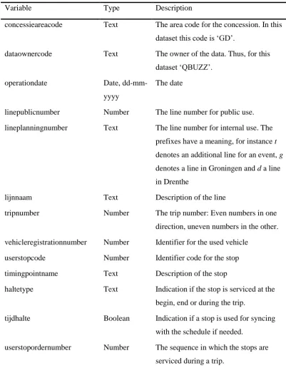
Table 4.2 lists the fields and their description as obtained from OV-bureau. An example of this data can be found in Appendix C. This dataset has to be

preprocessed in order to make it suitable for matching. For further processing, the dataset was loaded into a SQL table.

Variable Type Description

concessieareacode Text The area code for the concession. In this dataset this code is ‘GD’.

dataownercode Text The owner of the data. Thus, for this dataset ‘QBUZZ’.

operationdate Date,

dd-mm-yyyy

The date

linepublicnumber Number The line number for public use. lineplanningnumber Text The line number for internal use. The

prefixes have a meaning, for instance t

denotes an additional line for an event, g

denotes a line in Groningen and d a line in Drenthe

lijnnaam Text Description of the line

tripnumber Number The trip number: Even numbers in one

direction, uneven numbers in the other. vehicleregistrationnumber Number Identifier for the used vehicle

userstopcode Number Identifier code for the stop

timingpointname Text Description of the stop

haltetype Text Indication if the stop is serviced at the begin, end or during the trip.

tijdhalte Boolean Indication if a stop is used for syncing with the schedule if needed.

(41)

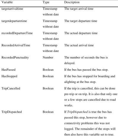
Variable Type Description targetarrivaltime Timestamp

without date

The target arrival time

targetdeparturetime Timestamp without date

The target departure time

recordedDepartureTime Timestamp without date

The actual departure time

RecordedArrivalTime Timestamp without date

The actual arrival time

RecordedPunctuality Number The number of seconds the bus is delayed.

HasPassed Boolean If the bus has passed the bus stop. HasStopped Boolean If the bus has stopped for boarding and

alighting at the bus stop.

TripCancelled Boolean If the trip is cancelled, this can be done pre-trip or on trip. It is also that only one or a few stops are cancelled due to road works.

[image:41.595.142.541.72.529.2]

TripDispatched Boolean If TripDispatched is true the bus has passed this stop, however due to connectivity problems this was not logged. The remainder of the stops will then also have this variable set to true.

Table 4.2: The fields of the bus data set as provided by OV-bureau

4.2.3 Data preprocessing

A few steps are needed before this dataset is ready for usage; First we rectify the noise in the data where possible. Next we trim the data in order to fit the study area and the time span. We conclude by augmenting the dataset with useful features

(42)

have to be converted to calendar dates before they can be used to append the target and recorded times. For most records this is rather easy; If a target time or a recorded time is between 00:00 and 04:00, the operation date plus 1 day should be added to the time, otherwise just the operation date is sufficient. Four bus lines start before 04:00 and end after 04:00. For these bus lines all the datetimes of the

records are increased with 1 day. These four bus lines are: 402 - Groningen - Vries [Nachtbus], 417 - Groningen - Roden - Leek [Nachtbus], 418 - Gieten - Groningen [Nachtbus] and 419 - Assen - Groningen [Nachtbus].

Also, the denotation of no recording for a departure time or arrival time was ambiguous. If there was no record these times were saved as '00:00:00' instead of a null value. Therefore, an extra step was needed to detect the records where

'00:00:00' was the actual recorded time.

Furthermore, the field 'recordedpunctuality', which represents the observed delay, is not reliable. Most often this variable describes the number of seconds between the planned departure time and the real departure time. However,

sometimes when the real departure time was missing, the recorded punctuality was based on the real arrival time. There are also lots of instances where there is a recorded punctuality, but no real arrival or departure time. For those instances the recorded departure time is calculated using the recorded punctuality and the target departure time.

There is noise in the data. The found anomalies are listed in Appendix D. Most anomalies are infrequent. However, it can be determined that the fields, especially those which are extracted from Koppelvlak 6,are not 100% reliable. These fields give feedback on how the bus executed the bus trip and are sent by the buses while on trip. It is not possible to precisely determine when the fields are erroneous. The occasions which are listed in the table stand out, because of the extremeness of the error. But less extreme errors are impossible to find easily and even when found it is unknown which field is erroneous. The biggest errors are rectified, but for the rest the dataset is used as is, while keeping in mind the possible errors in the data.

(43)

The dataset is augmented with the travel time since the last stop, the departure time of the last stop and the departure time of the next stop. The travel time since the last stop is used for exploratory data analysis. The departure time from the previous stop and the departure time at the next stop are used for the trip matching step as discussed later. The departure time is used since this is more frequently logged than the arrival time. If there is no recorded departure time available at the previous or next stop the target departure time is taken. In case the stop has no previous or next stop available the own recorded departure time was used plus or minus 30 minutes.

Moreover, the different datasets use different identifiers and aggregation levels for the stops. 9292 has defined the stops at one aggregation level higher in clusters, where stops with the same name are in the same cluster. For this analysis we will use the aggregation level used by 9292. Therefore, the records are also augmented with the 9292 stop clusters. The step where the bus data stops are matched to the 9292 clusters is described in Appendix F.

4.2.4 Data exploration

In this section we will highlight some key characteristics for this dataset.

(44)

[image:44.595.89.455.73.316.2]

Figure 4.2 Histogram of the recorded punctuality distribution for all recorded stop passages. X= punctuality, in seconds

Figure 4.3 Distribution of the recorded delay aggregated over hours

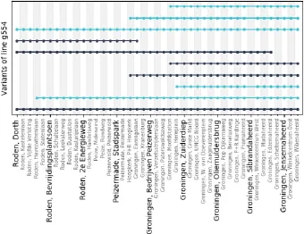
[image:44.595.91.376.365.682.2]

(45)

[image:45.595.170.511.236.498.2]

of lines as described in section 3.2.1. However, some lines do not have AVL data available or do not have a smart card reader device, for example lines which contain a belbus. These lines are later ignored. Unfortunately, most lines have a few trips that are serviced by a belbus, for instance in the off-peak period. This might provide problems since these trips provide noise to the dataset. Figure 4.4 shows an example of how the variants of a line are constructed: a variant is unique in the stops, stop order (implicitly also includes direction) and the line planning number.

Figure 4.4: Visualization for the different variants of line g554. The color of the line represents the direction and a node represents that the bus does service that stops. Some variants are longer as others.

(46)

[image:46.595.88.456.108.311.2]

own bin. The last bin (> 125 min) also contains the records without a headway, since a headway of over 125 is similar to the characteristics of the first trip.

Figure 4.5: The distribution of the headway.

4.3 Dataset 2 - Trip planner

We acquired a dataset from 9292 to use as trip planner usage data. The dataset contains the travel information consulted by users in their trip planner.

9292 is not the only travel planner in the Netherlands used for public transport freely available to the public. Among the biggest travel planners are 9292, NS, ANWB, Google Maps and Go About. The travel planners differ in looks, included modes which are included and functionality. Users choose a travel planner based on these differences and their personal preferences. For this case study we utilize data from the 9292-trip planner because is widely used and well known. It is specialized for public transport since 1992 and the data is available to us. We will therefore only discuss how users use the 9292-travel planner to plan their journey.

4.3.1 Description

The 9292-journey planner is an interactive trip planner which is accessible via internet on a web browser (www.9292.nl) or via an app for smartphone or tablet. In the trip planner you can plan a trip by public transport for all modes in the whole country. The planner requires an arrival or departure time and a start and end location as input from the user, see Figure 4.6 for the web-based version. The planner then searches for the most suitable (multimodal) journey by combining and comparing the public transport supply. The most suitable journey and its

alternatives are presented to the user via the interface as shown in Figure 4.7.

60

10 15

30

90 120

(47)

The best fitting journey is the first reasonably fast journey that starts after the time set as departure time or ends before the set arrival time. This journey is shown in an interface which also lists a few alternatives. These alternatives are presented as summaries with the departure and arrival time, the number of transfers and the total travel time. It is also shown if there are any delays or disruptions.

There are some extra options. The most apparent extra option is to add an intermediate destination. The trip planner will then plan a journey between the start and end destination via this intermediate destination. It is also possible to request 5 minutes extra transfer time, to exclude a travel mode (bus, train, light rail, metro or ferry) or to request for a journey that is wheelchair friendly.

Mulley et al. (2017) found the type and the use of travel information differed with the type of passengers, age and stage of the journey. E.g. older people are less aware of the available travel information sources. They also show that frequent travelers are more aware of the available information sources.

(48)

(49)

Figure 4.7 Travel suggestions in the web-based version of the 9292-trip planner. The interface has the following information blocks: a – the general travel information of the current option; b – button to show one option earlier; c – the four best results given the requests or after the user requested earlier (b) or later (d) options; d – same as b but for later options; e – extra information ("This travel option is no longer viable"); f – the detailed travel plan of the current active option; g – the current and planned times are shown both. Retrieved from

http://www.treinreiziger.nl/wp-content/uploads/2016/10/9292-reisadvies4a.jpg.

The motivation of the traveler for using the trip planner causes some typical (noise) patterns in the data. For instance, a potential traveler can use 9292 to see if his travel plans are even possible using public transport, or at what time the first and latest options are. In these cases, the potential traveler is only interested in the availability of a public transport connection at the time he or she needs it. This user will then enter a late (or early time) or use the current time and scroll through all the alternatives to find the latest (or earliest) departure time, whatever method he or she finds most convenient. At a later stadium this traveler might return to the planner to plan his journey in more detail. The requests in this case may be distinctive in time, where the check for possibility happens more than a day in advance and the detailed request happens a few hours in advance. However, in some cases this might be not the case.

a

b

c

d

e

(50)

Other purposes of using the trip planner are:

- To find the best possible travel plan (which minimizes the weighted utility cost function).

- To recheck an already chosen travel plan. For instance, to check their transfer times, transfer platforms, lines to transfer to, etc.

- To check if their delay causes problems later on in their multimodal journey.

- To check before leaving if there is any delay or disruptions.

- To find at what time the bus leaves every hour. Or to see if there is even an hourly pattern.

- To look if public transport is a competitor for transport by car.

- To adjust their travel plan during the trip because of disruptions or delays. - To look up historic journeys for declaration purposes.

Thus, based on the intended use, the number of requested alternatives and the interval between request time and departure time differs (well in advance, just before the trip, on trip, afterwards). Because the objective is to predict the number of people boarding in advance, we only can use the requests made pre-trip. This check has to be done per part of the multimodal journey. For instance, if a travel advice consists of two journey parts connected by a transfer, the request can be made on trip for the first part and pre-trip for the other.

It should be noted, that you can classify the travel requests in different ways. One way is by the objective of the user, another could be by looking at what stage in the trip the traveler boards the bus. If the traveler first has to travel 200

kilometers by 3 different trains, there is a chance that he misses a transfer or that the train is delayed. In this case the ridership of this particular bus is dependent on the trains by which it is connected. So there could be less predictive power in requests in which the bus is the last leg in a multimodal/multivehicle trip.

Furthermore, the predictive power in a trip with the mode bus as the first leg could be as high as a trip in which the bus is the only motorized mode.

Thus, different kinds of noise are bound to occur in the dataset due to the design, usage and human error.

4.3.2 Data collection

Each time a travel plan is shown (e.g. after the initial search or each time the user selects an alternative), data are logged. For each such occurrence, the

(51)

parts. Figure 4.8 shows an example of the difference between the total journey and the journey parts. These data are logged in two separate tables – journeyquestions

(Table 4.3) and journeyparts (Table 4.4) - which are linked with the field

question_tulp_id. Thus, data is available for the chained trip as well as for the individual parts.

Figure 4.8: Difference between a journey question and its journey parts. For the example the actual advice for a journey between the office of OV-bureau in Assen and the office of Qbuzz in Groningen is used.

The data acquired to perform this research is collected from the APP, the website and the API. The custom requests made by travelers by calling the 9292-call center are also present because the operatives use the website to gather the travel recommendation. The API is used by some other online travel planners like the travel planner from Qbuzz. These other travel planners can have a different design or a somewhat different functionality. This can result in other typical usages and thus data characteristics.

Some of these data are made available for this case study. The data are supplied by 9292 via two connected tables which are displayed in Table 4.3 and Table 4.4. Appendix C shows a raw sample from these two tables.

Field Type Description

question_tulp_id Text A GUID (Globally Unique Identifier) to denote the question.

planner Text

action Text

request_datetime Date with time

The date and time the request was made rounded to minutes.

departuredatetime Date with time

The date and time of departure for the suggested (multimodal) journey.

Forecasting bus ridership with trip planner usage data : a machine learning application