Development of approaches for screening antimalarial compounds based on their modes of action

warwick.ac.uk/lib-publications

A Thesis Submitted for the Degree of PhD at the University of Warwick

Permanent WRAP URL:

http://wrap.warwick.ac.uk/87913

Copyright and reuse:

This thesis is made available online and is protected by original copyright.

Please scroll down to view the document itself.

Please refer to the repository record for this item for information to help you to cite it.

Our policy information is available from the repository home page.

M A E

G

NS I

T A T MOLEM

U N

IV

ER

SITAS WARWICEN

SIS

Development of Approaches for Screening

Antimalarial Compounds Based on Their Modes of

Action

by

Arturas Grauslys

Thesis

Submitted to the University of Warwick

for the degree of

Doctor of Philosophy

Systems Biology DTC

Contents

List of Tables v

List of Figures vi

Acknowledgments xi

Declarations xii

Abstract xiii

Abbreviations xv

Chapter 1 Introduction 1

1.1 Malaria . . . 1

1.1.1 The Deadliest Strain . . . 1

1.1.2 Prevention and Treatment . . . 3

1.1.3 Drug Discovery . . . 5

1.2 Aims of The Study . . . 6

1.3 Metabolomics . . . 7

1.3.1 Analytic Techniques and Applications . . . 8

1.3.2 Metabolomics in Drug Discovery . . . 10

1.4 Fourier Transform Infrared Spectroscopy . . . 12

1.4.1 Working Principles Behind FT-IR . . . 12

1.4.2 Data Acquisition and Analysis . . . 14

1.5 Nuclear Magnetic Resonance Spectroscopy . . . 16

1.5.1 Working Principles Behind NMR . . . 16

1.5.2 An NMR Experiment . . . 21

1.6 High Content Imaging . . . 25

1.6.1 HCI Experiments and Data Collection . . . 26

1.7.1 Principal Component Analysis . . . 27

1.7.2 Linear Discriminant Analysis of Principal Components . . . . 28

1.7.3 Partial Least Squares Discriminant Analysis . . . 29

1.7.4 Permutation Test . . . 30

1.7.5 Hierarchical Clustering . . . 31

1.7.6 Multiple Dataset Integration . . . 32

Chapter 2 Materials and Methods 33 2.1 Parasite Cultures . . . 33

2.1.1 Culture Medium . . . 33

2.1.2 Uninfected Red Blood Cells . . . 34

2.1.3 Gas Phase . . . 34

2.1.4 Parasite Synchronisation . . . 35

2.1.5 Estimation of Parasitemia . . . 35

2.1.6 Haemocytometry . . . 36

2.1.7 Magnetic Separation of Infected Erythrocytes . . . 36

2.1.8 Cryopreservation of Parasites . . . 36

2.1.9 Determination of IC50 Concentrations of Drugs . . . 37

2.2 Experimental Procedures for FT-IR Metabolomics Experiments . . . 39

2.2.1 Sample Preparation . . . 39

2.2.2 Sampling at T=0 h and Time-Course Set-up . . . 39

2.2.3 Sampling at Later Time-points . . . 40

2.2.4 FTIR Readings . . . 40

2.3 Experimental Procedures for NMR Metabolomics Experiments . . . 40

2.3.1 Drug Exposure Time-Course Setup . . . 41

2.3.2 Sampling . . . 42

2.3.3 Metabolite Extraction . . . 42

2.3.4 Lyophilisation . . . 43

2.3.5 Sample Preparation For NMR Readings . . . 44

2.3.6 NMR Parameter Set-up . . . 44

2.4 Experimental procedures for High Content Imaging Study . . . 44

2.4.1 Experimental Set-up . . . 45

2.4.2 Data Acquisition and Processing . . . 45

2.5 Data Analysis . . . 47

2.5.1 FTIR Data Analysis . . . 47

2.5.2 NMR Data Analysis . . . 48

Chapter 3 Method Development 51

3.1 Introduction . . . 51

3.2 Determination of Optimal RBC Count for FT-IR Experiments . . . 52

3.3 Signal Maximisation in NMR Experiments ofP. falciparum Infected RBCs. . . 53

3.4 Development of Sample Preparation Procedures for NMR Experiments 55 3.4.1 Optimisation of Metabolite Extraction Protocol . . . 56

3.4.2 Comparison of Metabolite Extraction Solutions . . . 58

3.4.3 Comparison of Sample Drying Methods . . . 59

3.4.4 Optimization of Sample Size . . . 60

3.5 Determination of Optimal NMR Parameter Set . . . 68

3.5.1 Introduction of CPMG Pulse Sequence . . . 68

3.5.2 Quality Control and Resolution Increase . . . 69

Chapter 4 ProcNMR - Custom NMR Data Processing Software 72 4.1 Introduction . . . 72

4.2 Motivation and Alternatives . . . 73

4.3 Functionality . . . 74

4.4 Implementation Details . . . 78

4.5 Further Develoment . . . 83

Chapter 5 Metabolic Fingerprinting of P. falciparum Using FT-IR Spectroscopy 84 5.1 Introduction . . . 84

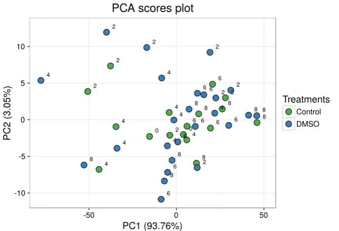
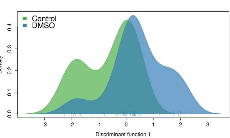
5.2 Study of the Effects of DMSO on RBCs . . . 84

5.3 Discrimination BetweenP. falciparum Infected and Uninfected RBCs 86 5.4 Discrimination Between Infected RBCs At Various Stages of the P. falciparum Life-cycle . . . 89

5.5 Discussion . . . 91

Chapter 6 The Effect of Drug Exposure to the Metabolome of P. falciparum: an NMR Spectroscopy Study 93 6.1 Introduction . . . 93

6.2 5-Hour Drug Exposure Study . . . 94

6.2.1 A repeat of the 5-hour study . . . 95

6.2.2 Further Optimization of the Experimental Procedure . . . 99

6.2.3 A Test of Drug Viability . . . 100

6.2.5 20-Hour Drug Exposure . . . 103

6.3 Re-interrogation of Short Time-course Drug Exposures . . . 106

6.3.1 The 6-Hour Time-Course . . . 106

6.4 Full Life-Cycle Drug Exposures . . . 111

6.5 Modeling Time-course data . . . 122

6.6 Discussion . . . 123

Chapter 7 High Content Imaging Study of P. falciparum Phenotype After Exposure To Antimalarial Compounds. 128 7.1 Study Design . . . 129

7.2 Data Processing and Analysis . . . 132

7.3 Discussion . . . 139

Chapter 8 Conclusions 141

Appendix A NMR spectra of ring and trophozoite life cycle stages of

List of Tables

1.1 Tentative assignment of bands frequently found in biological FT-IR spectra. . . 15

2.1 Drugs used in NMR experiments. . . 41 2.2 The measurements of the cell nucleus selections in the Harmony

soft-ware. . . 46 2.3 The Image analysis constraints on the selected field inclusion in the

dataset. . . 46

4.1 The functions performed by ProcNMR pipeline. . . 75

6.1 TheIC50values for the antimalarials used in the study obtained from a standard SYBR green assay. . . 100

7.1 The antimalarial drugs used in the imaging study. . . 129 7.2 The p-values from permutation tests in each experiment rounded to

List of Figures

1.1 A schematic illustration of the life-cycle ofP. falciparum . . . 2 1.2 A schematic illustration of the FT-IR spectrometer. . . 13 1.3 An example interferogram from an FT-IR reading. . . 14 1.4 Schematic illustration of the flip of magnetisation vectors of nuclear

spins through application of a radiofrequency pulse in the NMR probe. 19 1.5 Schematic illustration of magnetisation vector synchronisation after

the application of the radiofrequency pulse. . . 20

2.1 96-well plate setup for determination of drug IC50concentrations. . . 38 2.2 A standard 6-well plate set-up. . . 41 2.3 A schematic of metabolite extraction procedure. . . 43 2.4 The shapes of texture features detected by the Laws filters in the

Harmony softare. . . 47 2.5 A schematic illustration of the model training, testing and validation

approach employed for image analysis. . . 50

3.1 FTIR spectra acquired from a 2-fold serial dilutions of RBCs starting with 1.7 million cells as the initial count. . . 53 3.2 1D 1H NMR spectra of P. falciparum infected RBC samples,

ex-tracted using ice-cold 1:1 methanol and water and 2:2:1 acetonitrile, methanol and water. . . 57 3.3 A comparison of two 1D 1H NMR spectra of P. falciparum infected

RBC samples, extracted using 1:1 methanol and water and 2:2:1 ace-tonitrile, methanol and water. . . 62 3.4 A comparison of two 1D 1H NMR spectra of P. falciparum infected

3.5 PCA scores plot of the NMR experiment carried out using two differ-ent metabolite extraction approaches and two differdiffer-ent sample drying

methods. . . 64

3.6 A PCA scores plot of the NMR experiment carried out using two different metabolite extraction approaches and two different sample drying methods. . . 65

3.7 A PCA scores plot of the NMR spectra acquired from an experiment carried out on various stages ofP. falciparum parasites life cycle and at different volumes of culture used per sample. . . 66

3.8 A comparison of three 1D 1H NMR spectra acquired from P. falci-parum infected RBC metabolite extracts, using various volumes of cell pellet. . . 67

3.9 A comparison of 1D 1H NMR spectra acquired from P. falciparum infected RBC metabolite extracts, using two different pulse sequences: NOESY and CPMG. . . 70

3.10 A comparison of 1D 1H NMR spectra acquired from P. falciparum infected RBC metabolite extracts, using two different spectrometers: 600 MHz and 800 MHz. . . 71

4.1 Example output of a ProcNMR run. . . 76

4.2 Example output of a ProcNMR configuration tool run. . . 77

4.3 Schematic illustration of ProcNMR Workflow . . . 79

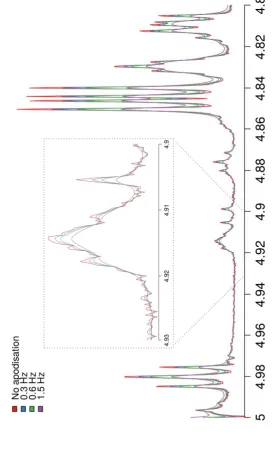
4.4 Example of effects of exponential apodisation applied with a range of values of the line broadening parameter (lb). . . 81

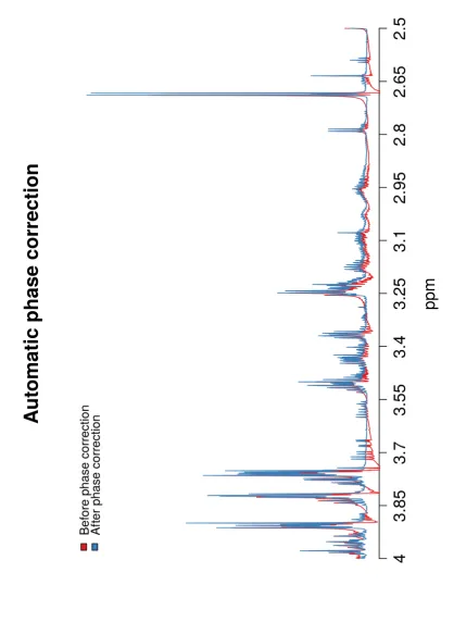
4.5 An overlay of a spectra before and after automatic phase correction in ProcNMR. . . 82

5.1 PCA scatterplot of an FTIR experiment testing DMSO effects on the RBCs. . . 85

5.2 DA-PC density plot on the first discriminant function. . . 86

5.3 PCA scatterplot of the FTIR experiment comparing infected and un-infected RBCs. . . 87

5.4 DA-PC density plot of the comparison between infected and unin-fected RBC data from an FTIR experiment. . . 88

5.5 The loadings plot of the DA-PC shown in Fig. 5.4. . . 89

5.7 DA-PC plot of the first two discriminant functions of the FTIR exper-iment comparing RBCs infected with various stages ofP. falciparum. 91

6.1 PCA of1H NMR spectra collected fromP. falciparum infected RBC samples after 5-hour drug exposure. . . 95 6.2 PCA of1H NMR spectra collected fromP. falciparum infected RBC

samples after 5 hour drug exposure. . . 96 6.3 PCA of1H NMR spectra collected fromP. falciparum infected RBC

samples after 5 hour drug exposure. . . 97 6.4 PCA of1H NMR spectra collected fromP. falciparum infected RBC

samples after 5 hour drug exposure. . . 98 6.5 PCA of1H NMR spectra collected fromP. falciparum infected RBC

samples after 5 hour drug exposure. . . 99 6.6 PCA of1H NMR spectra collected fromP. falciparum infected RBC

samples after 5 hour drug exposure atIC90 drug concentrations. . . 101 6.7 PCA of1H NMR spectra collected fromP. falciparum infected RBC

samples after 5 hour drug exposure at 10×IC90drug concentrations. 102 6.8 PCA of1_{H NMR spectra collected fromP. falciparum infected RBC}

samples after 5 hour drug exposure at 10×IC90drug concentrations. 103 6.9 PCA of1H NMR spectra collected fromP. falciparum infected RBC

samples after 5 and 20 hour drug exposure at 10×IC90 drug concen-trations. . . 104 6.10 PCA of 1H NMR spectra of medium samples collected from P.

fal-ciparum 20 hour drug exposure experiment using 10 ×IC90 drug concentrations. . . 105 6.11 PCA of 1H NMR spectra collected fromP. falciparum infected RBC

samples after 2, 4 and 6 hours of drug exposure at 10×IC90 concen-trations. . . 107 6.12 PCA of 1H NMR spectra collected from medium samples ofP.

falci-paruminfected RBC drug exposure experiment 2, 4 and 6 hours after the start of the exposure. . . 108 6.13 PCA of 1H NMR spectra collected fromP. falciparum infected RBC

samples after 2, 4 and 6 hours of drug exposure at 10×IC90 concen-trations. . . 109 6.14 PCA of 1H NMR spectra collected fromP. falciparum infected RBC

6.15 PCA of 1H NMR spectra collected fromP. falciparum infected RBC samples after 2, 4 and 6 hours of drug exposure at 10×IC90

concen-trations. . . 111

6.16 A quantile plot of 1H NMR spectra collected from a P. falciparum drug exposure experiment after 3 hours of exposure. . . 113

6.17 A quantile plot of 1H NMR spectra collected from a P. falciparum drug exposure experiment after 6 and 12 hours of exposure. . . 114

6.18 A quantile plot of 1H NMR spectra collected from a P. falciparum drug exposure experiment after 24 hours of exposure. . . 115

6.19 PCA of 1H NMR spectra collected fromP. falciparum infected RBC samples after 3, 6, 12, 24 and 48 hours of drug exposure at IC90 concentrations. . . 116

6.20 PCA of1H NMR spectra collected from RBC samples after 3, 6, 12, 24 and 48 hours of drug exposure atIC90 concentrations. . . 117

6.21 PCA of 1H NMR spectra collected fromP. falciparum infected RBC samples after 3, 6, 12, 24 and 48 hours of drug exposure at IC90 concentrations. . . 118

6.22 HCA dendrogram of 1H NMR spectra collected from P. falciparum infected RBC samples after 3, 6, 12, 24 and 48 hours of drug exposure atIC90 concentrations. . . 119

6.23 HCA dendrogram of 1H NMR spectra collected from RBC samples after 3, 6, 12, 24 and 48 hours of drug exposure atIC90concentrations.120 6.24 HCA dendrogram of 1_{H NMR spectra collected from P. falciparum} infected RBC samples after 3, 6, 12, 24 and 48 hours of drug exposure atIC90 concentrations. . . 121

6.25 MDI cluster dependency heatmaps. . . 123

7.1 Images of infected red blood cells in Giemsa-stained smears. . . 131

7.2 Fluorescent images ofP. falciparum infected RBCs. . . 133

7.3 Example scatterplots of four wells from one of the imaging plates. . 134

7.4 Example scatterplots of four wells from one of the imaging plates. . 135

7.5 A histogram representing the empirical distribution ofQ2 values cal-culated in a permutation test using PLS-DA models fitted to two groups of treatments. . . 136

7.7 MeanQ2 values for each ensemble of 20 models fitted to experiment data. . . 138

A.1 1D 1H NMR spectra of RBC samples infected with P. falciparum at ring and trophozoite stage, extracted using ice-cold 1:1 methanol and water and 2:2:1 acetonitrile, methanol and water. . . 168 A.2 1D 1H NMR spectra of RBC samples infected with P. falciparum at

ring and trophozoite stage, extracted using ice-cold 1:1 methanol and water and 2:2:1 acetonitrile, methanol and water. . . 169 A.3 1D 1H NMR spectra of RBC samples infected with P. falciparum at

ring and trophozoite stage, extracted using ice-cold 1:1 methanol and water and 2:2:1 acetonitrile, methanol and water. . . 170 A.4 1D 1H NMR spectra of RBC samples infected with P. falciparum at

ring and trophozoite stage, extracted using ice-cold 1:1 methanol and water and 2:2:1 acetonitrile, methanol and water. . . 171 A.5 Quantile plot of 1D 1H NMR spectra of RBC samples infected with

P. falciparum at ring and trophozoite stage, extracted using ice-cold 1:1 methanol and water and 2:2:1 acetonitrile, methanol and water. . 172 A.6 Quantile plot of 1D 1H NMR spectra of RBC samples infected with

P. falciparum at ring and trophozoite stage, extracted using ice-cold 1:1 methanol and water and 2:2:1 acetonitrile, methanol and water. . 173 A.7 Quantile plot of 1D 1H NMR spectra of RBC samples infected with

P. falciparum at ring and trophozoite stage, extracted using ice-cold 1:1 methanol and water and 2:2:1 acetonitrile, methanol and water. . 174 A.8 Quantile plot of 1D 1H NMR spectra of RBC samples infected with

Acknowledgments

It would be hard to count all the people that have played a part in the successful

completion of my PhD project. I am sure I will forget some, but I’m sincerely

thankful to everyone nonetheless. First I would like to thank my PhD advisors:

prof. David Wild and prof. Steve Ward. Besides their invaluable advice they

always trusted my judgement and allowed me freedom I could not have expected.

They did not just help me develop the skills for science but also independence and

initiative. My supervisors were instrumental in the success of my work, however

it is hard to overestimate the help of all the people around me that shared their

knowledge and advice day-to-day. Dr. Felicity Curie was a great teacher to me at

the very beginning. She was always first to offer ideas and stress scientific rigor

above everything else. I am grateful for numerous inspiring discussions we had that

left me thinking and that were the most rewading. I’m thankful to Dr. Marie

Phelan, who persevered through my countless trials and errors. Who was always

there with her advice, encouragement and optimism. I would like to express my love

and gratitude to my parents Laimute and Algis, who have always supported me with

love and patience, who were always on my side even when they did not agree with

my decisions, and always had the words I needed to hear. To my younger siter

Lina I want to say many thanks for her encouragement, inspirationa and her sense

of humour regardless of the situation. But most importantly my greatest love and

earnest gratitude to Eva - my wonderful partner in life and science. For her support

and encouragement, advice and lessons, honest criticism, and for countless hours

spent helping me I am forever in her debt. This work would truly be impossible

Declarations

Research presented in this thesis is completely original and my own, with exception

of where acknowledged below. I confirm that this thesis has not been submitted

for another degree at any other University. NMR spectroscopy parameter set up

used for experiments presented in Chapter 6 were selected by Dr. Marie Phelan,

Shared Research Facility Manager of the NMR Centre at the University of Liverpool.

Cellular extractions performed in experiments presented in Chapter 6 were collected

with the assistance of Eva Caamano-Gutierrez. Drug exposure assays and high

content imaging analyses presented in Chapter 7 were performed with the assistance

Abstract

Malaria is an infectious tropical disease responsible for hundreds of thousands of

deaths every year. It is caused by a parasite from genusPlasmodium of which

fal-ciparum is the most deadly and the focus of this study. The limited number of

currently available drugs are further threatened by the rising frequency of

resis-tance. This has greatly emphasised the need for new drugs with novel modes of

action. The current drug development pipelines rely on large scale compound

li-brary screens for antimalarial effect. Computational chemometric methods are then

used for selecting promising hits for further investigation. Such analyses however

rely on indirect characterisation of compound effects. In this project we

investi-gated three approaches aimed at developing compound screening assays based on

compound effects on live cells. The first two approaches relied on metabolomics

techniques. Based on the assumption that the drug induced metabolic changes in

the malaria parasite could be uniquely assigned to the drug mode of action we

hypothesised that if such metabolic states could be measured they could be used

to cluster the compunds into groups based on their modes of action. By

compar-ison to well established antimalarials the clusters of novel compounds could then

be characterised and novel compound clusters identified. The third method relied

on the phenotypic information for drug exposed malaria parasites derived from the

analysis of fluorescent microscopy images. This assay aimed at characterising the

modes of action of the compounds as well as the speed of kill. The first method

investigated was based on metabolic fingerprinting using Fourier transform infrared

spectroscopy. The sample preparation and data acquisition protocols were

insufficient for the detection of drug induced effects in P. falciparum. Next a

nu-clear magnetic resonance (NMR) spectroscopy-based method was developed. While

the method was promising in terms of high throughput capabilities, consistency and

the breadth of information posed a series of issues, mainly associated with

sensi-tivity. In the absence of a suitable automated data processing solution a custom

software “ProcNMR” was developed and used to process the data collected in the

experiments. A full experimental procedure was developed and tested, however the

NMR sensitivity issues, exacerbated by the complex intraerythrocytic nature ofP.

falciparum resulted in suboptimal outputs. Lastly a high content imaging-based

technique was investigated. Data processing and predictive analysis methods were

developed and implemented. A pilot experiment was used to demonstrate the

po-tential of the technique to discriminate between fast and slow acting drugs. The

compounds of the “Malaria Box” were screened using this technique and a gorup of

Abbreviations

1D One-dimensional

2D Two-dimensional

ACT Artemisinin-based combination therapy

ADC Analog-to-digital converter

AQ Amodiaquine

AT Artemisinin

ATO Atovaquone

CE Capillary electrophoresis

CM Complete medium

COSY Correlation spectroscopy

CPMG Carr-Purcell-Meiboom-Gill

CQ Chloroquine

DALY Disability-adjusted life-years

DA-PC Discriminant analysis of principal components

DHFR Dihydrofolate reductase

DMPK Drug metabolism and pharmakokinetics

FA Fusidic acid

FID Free induction decay

FIR Far infrared

FT-IR Fourier-transform infrared spectroscopy

GC Gas cromatography

GSK GlaxoSmithKline

HCI High content imaging

HSQC Heteronuclear single quantum correlation

IC50 Half maximal inhibitory concentration

IR Infrared

iRBC Infected red blood cell

KO Knock-out

LC Liquid chromatography

LDA Linear discriminant analysis

MIR Mid-wavelength infrared

MMV Medicines for Malaria Venture

MS Mass spectrometry

NCBI National Centre for Biotechnology Information

NIR Near infrared

NMR Nuclear magnetic resonance

NOESY Nuclear Overhauser effect spectroscopy

P Plasmodium

PC Principal component

PCA Principal component analysis

PG Proguanil

PLS Partial least squares

PLS-DA Partial least squares discriminant analysis

QCDs Quinoline containing drugs

RBC Red blood cell

ROS Reactive oxygen species

RPMI Roswell Park Memorial Institute medium

SEM Standard error of the mean

STOCSY Statistical total correlation spectroscopy

TCA Trycarboxylic acid cycle

TMS Tetramethylsilane

TSP 3-(Trimethylsilyl) propionic acid

vs Versus

WHO World Health Organisation

Chapter 1

Introduction

1.1

Malaria

Malaria is an infectious tropical disease caused by parasites of the genusPlasmodium. There are five species that cause disease in man: Plasmodium falciparum,malariae, vivax, ovale and knowlesi. Parasites are transmitted to humans through the bite of a female mosquito of genus Anopheles. There are up to 800 million cases of malaria every year in tropical and subtropical regions including sub-Saharan Africa, Southeast Asia, Oceania and some regions of Central America. Of those about 500,000 cases end in death from severe complications, especially among children and pregnant women [WHO, 2014]. The global burden of malaria in disability-adjusted life-years (DALY) as quoted by Hotez et al. [2014] is 83 million, where DALY is a number of years lost due to disability or early death caused by a disease. While the most prevalent strain ofPlasmodiumisP. vivax the most of the deaths from malaria are in cases of infection with P. falciparum [WHO, 2014]. It is distinguished from other strains by its ability to infect erythrocytes of any age allowing parasitemia of up to 80% as well as the production of proteins that facilitate red blood cell (RBC) binding to endothelial cells on capillaries - sequestration - especially in the brain, causing a range of severe complications including bleeding, seizures and coma [Rowe et al., 2009].

1.1.1 The Deadliest Strain

has a 42-53 hour life-cycle depending on the growth conditions (Fig. 1.1).

Figure 1.1: A schematic illustration of the lifer-cycle ofP. falciparum (source: Klein [2013])

protein adhesins on the erythrocyte membrane that allow the red blood cells to bind to the endothelial cells in the host microcirculation. The process is called sequestration and protects the infected RBCs from removal from the bloodstream by the spleen. The parasites spend the last 24-34 hours of their development in this state. During this time they develop into schizonts and produce on average 16 merozoites each. Once the parasites are fully mature the RBC is ruptured, the merozoites enter the bloodstream and infect new RBCs. The cycle continues subsequently raising the the level of parasitemia up to 20 times every 48 hours. Some of the parasites do not go through the asexual replication cycle and instead develop into sexual stages - gametocytes. The gametocytes, when ingested by a mosquito during a bloodmeal, undergo gametogenesis that result in formation of micro- and macrogametes. Microgametes fertilize macrogametes that result in formation of zygotes and subsequently oocysts. Through asexual replication oocysts produce sporozoites thus completing the life-cycle of Plasmodium. Almost any part of this life cycle can be targeted by treatment and prevention measures. The exclusive focus of this thesis will be the asexual intra-erythrocytic part of theP. falciparum life-cycle, the life cycle stage associated with the clinical manifestations of malaria.

1.1.2 Prevention and Treatment

The fight against malaria has been ongoing since the formal discovery of the disease at the end of the nineteenth century [Cox, 2010]. The efforts towards eradication of malaria have been divided between vaccine development, vector control and treat-ment of infection.

that can often lead to morbidity and death. Currently available antimalarial drugs can be classified into four main categories: quinoline-like compounds; artemisinins; mitochondrial inhibitors, of which atovaquone is the only one available; and antifo-lates. Some antibacterial compounds, including sulfones, macrolides, tetracyclins, lincosamides and chloramphenicol have antimalarial activity but are rarely used and only ever in combination with other more active compounds.

Quinoline-like compounds including quinine, chloroquine (CQ), amodiaquine,

piperaquine, mefloquine and others act by inhibiting haem detoxification within the asexual parasite food vacuole e.g. chloroquine binds to heamoglobin degradation products, inhibits haem dimerisation and hemozoin formation. The heam toxicity is therefore the explanation of the mode of action of quinolines [Fitch, 2004].

Artemisinins are endoperoxides derived from a natural product found in the

Artemisia annua plant. They are fast acting compounds capable of affecting the broadest range of the parasite asexual life cycle. There are a range of artemisinins currently in use including artemether, dihydroartemisinin and artesunate. The exact mode of action of the artemisinins is still controversial, although it is thought that it could be linked to iron-dependent cleavage of the unique endoperoxide bridge, triggering formation of carbon-based radicals and epoxides that then target essential parasite macromolecules generating drug adducts [Olliaro et al., 2001].

Atovaquone inhibits the parasite electron transport chain by targeting the

cy-tochrome bc1 complex. This results in the collapse of the mitochondrial membrane potential and inhibition of pyrimidine biosynthesis [Srivastava et al., 1997].

Antifolates including pyrimethamine, cycloguanil and trimethoprim interfere with

pyrimidine synthesis in P. falciparum by inhibition of dihydrofolate reductase -thymidylate synthase (DHFR) [Muller and Hyde, 2010].

quinolines - mefloquine and quinine [Price et al., 2004; Nkrumah et al., 2009]. The efficacy of antifolates is reduced up to 1000-fold by a mutations in DHFR (N51I, C59R, S108N) and DHPF (A437G,K540E) genes that reduce the binding affin-ity of the drug [Gregson and Plowe, 2005]. Resistance to atovaquone arises from point-mutations (N268N/S/C) in the cytochrome-b encoding gene [Srivastava et al., 1999]. Artemisinin resistance has emerged in recent years and is reported to be as-sociated with mutations in theP. falciparum proteinkelchencoded on chromosome 13 [Ariey et al., 2014; Takala-Harrison et al., 2015]. Artemisinin combination thera-pies are currently the preferred treatment for malaria worldwide. While artemisinin monotherapies are now not recommended and are being gradually phased out fol-lowing the WHO recommendations [WHO, 2015] the emergence of artemisinin re-sistance threatens the efficacy of combination therapies as well.

1.1.3 Drug Discovery

Resistance to antimalarial drugs has been rising since the 1960s and now blights all available drug classes having a major impact on malaria control and treatment ef-forts worldwide. The only solution to this problem is the discovery of new drugs with unique mechanisms of action. Today new antimalarial drug discovery is a world-wide effort led mainly by a few private-public organisations including the Medicines for Malaria Venture (www.mmv.com) as well as the Drugs for Neglected Diseases initiative (www.dndi.org).

for efficacy in live cells, acceptable toxicity margins and good drug metabolism and pharmacokinetics (DMPK) including adequate oral bioavailability [Flannery et al., 2013]. For example, cysteine proteases such as falcipains are vital to Plasmod-ium life cycle [Rosenthal, 2011] and nonspecific inhibitors of cysteine proteases are effective against the parasite [Joachimiak et al., 2001], however none of the poten-tial compounds that target this pathway have successfully reached the clinic due to problems with toxicity as well as poor pharmacokinetics. Development of high thoughput whole cell screens has allowed rapid identification of novel compounds in high numbers [Plouffe et al., 2008]. Such compounds have guaranteed activity against the parasites without any detailed understanding of their targets or modes of action. Millions of compounds have been screened in whole-cell assays in recent years. The effort was led by St. Jude Children Hospital who screened 300,000 com-pounds against P. falciparum [Guiguemde et al., 2010], GlaxoSmithKline (GSK) screening over 2,000,000 compounds [Gamo et al., 2010] and an academic/industry consortium led by Novartis that screened over 800,000 compounds [Rottmann et al., 2010; Plouffe et al., 2008]. These screens have resulted in the identification of thou-sands of compounds with activity againstPlasmodium that have been collected in the ChEMBL repository for medicinal chemistry data directed at neglected tropical diseases (http://www.ebi.ac.uk/chemblntd). Due to obvious restrictions in financial and time cost the vast number of hits requires a further selection of compounds for more detailed study. Such an triaging effort was carried out by MMV in the gener-ation of the “Malaria Box”, a selected set of validated hits that are recommended for further investigation [Spangenberg et al., 2013]. The “Malaria Box” includes 400 compounds that have been selected in two categories: drug-like compounds and probe-like compounds. These compounds are publicly available on request from the MMV as is a newer screening compound set called the “Pathogen Box”.

1.2

Aims of The Study

under-standing of currently used compounds as well allowing selection of compounds with novel mode of action. This thesis is focused on the study of strategies that can help classify antimalarial hits based on their mode of action.

In order to classify compounds by mechanism a metabolomic fingerprinting approach was chosen. This choice was made based on a series of assumptions. Firstly it was assumed thatP. falciparum has a finite number of druggable targets. This assumption implies that if there are more effective compounds than potential targets there is redundancy in the compound set that should allow clustering based on mechanism. It was also assumed that drugs with different modes of action induce different metabolic perturbations in the parasite leading to arrest of development or death. If those metabolic states could be identified and uniquely assigned to the modes of action they could serve as a proxy for compound classification.

The metabolic fingerprinting approach was chosen for the measurement of the global metabolic state in the parasite after exposure to compounds. A series of currently used compounds will be first employed in order to develop and validate the method followed by experiments involving the “Malaria Box” compounds with unknown mechanism. The data collected from experiments using well-understood antimalarial drugs as probes will generate the framework against which the clus-tering structure of the unknown compounds can be evaluated, highlighting clusters with novel modes of action.

1.3

Metabolomics

mem-ber of the ’-omics’ family together with genomics, transcriptomics and proteomics. It is often seen as arguably being “closer to phenotype” subject of study. Significant changes at the metabolite level have been demonstrated to be possible even when changes in transcript or protein concentrations are relatively low [Kell and Mendes, 2000]. Metabolomics in the most general sense is a global discovery science. In many cases analysis starts without a hypothesis and aims at identifying “points of interest” around which hypotheses can be built. Depending on the aims of the study, the analysis can take one of a few configurations including (a) fingerprinting, (b) footprinting, (c) profiling, (d) flux analysis and (e) targeted analysis. Metabolic fingerprinting is a global investigation of all measurable metabolites in the system without identification or quantification. It is usually performed for comparison of system metabolic states under different conditions. Footprinting is fingerprinting of the metabolome outside of the targeted system or the environment of the system and is usually performed for investigation of metabolite exchange. Metabolome profiling includes identification of metabolites and relative quantification in order to estab-lish an interpretable profile of the metabolome under specific conditions. Tracing isotope labelled molecules allows flux analysis of metabolites in the target system and between the system and its environment. Targeted metabolomics usually refers to identification and absolute quantification of pre-specified metabolites in order to quantitatively characterise the effects of treatments or experimental conditions at the metabolic pathway level. All of these methods of study of the metabolome are only possible because of the progress in analytic platforms as well as the associated data analysis techniques.

1.3.1 Analytic Techniques and Applications

In principle collection of metabolomics data is a complex task. Metabolites in a biological system include a wide range of organic compounds such as nucleotides, amino acids, vitamins, hormones and other signalling molecules. There is no single analytic technique that would be able to quantify or even detect all the metabolites in the system. A range of analytic techniques have been adopted including Fourier transform infrared spectroscopy (FT-IR) and Raman spectroscopy, nuclear magnetic resonance (NMR) spectroscopy and mass spectrometry (MS) in metabolomic studies in order to acquire data appropriate for the aims of the study.

that is not absorbed is detected and the absorbance spectrum is obtained. The absorption pattern then can be correlated to the chemical species present in the sample [Stuart, 2006]. This forms a spectrum that can be unique to the sample like a “fingerprint”. While FT-IR is not as sensitive as other spectroscopic tech-niques such as mass spectrometry, its high throughput and reproducibility are seen as valuable advantages in a wide range of applications such as biomarker discov-ery [Harrigan and Goodacre, 2003], food science [Ellis et al., 2002] and bacterial metabolism studies [Kaderbhai et al., 2003]. Raman spectroscopy is different from FT-IR with the exchange of energy from a source is measured usually in the visible part of the electromagnetic spectrum. The Raman shift in energy of the light is observed that is traceable to specific chemical species. The advantage of Raman spectroscopy over FT-IR is that the water signal is not present and therefore the samples can be in tissue, in solution or even in vivo [Hata et al., 2000; Buschman et al., 2000; Yu et al., 2006]. The main limitation of Raman spectroscopy is that the Raman effect is weak and therefore the sensitivity of the technique is low compared to FT-IR.

other spectroscopic approaches. Firstly the relatively low sensitivity is compensated by very high reproducibility [Keun et al., 2002]. It requires small volume of sample and, in case of biofluids such as urine, blood plasma or cerebrospinal fluid, requires little sample preparation. It is also non-destructive and has relatively fast data ac-quisition. Due to non-destructive nature of the technique it allows other analyses to be performed on the same samples. No prior knowledge of the sample contents or separation steps (as in case of MS) is required. The samples can be analysed in an exploratory manner and sample contents inferred from the resulting data. For these reasons NMR is often used in untargeted metabolomics studies such as finger-printing or footfinger-printing where simple discrimination between samples from different treatments or experimental conditions is desired.

Mass spectrometry (MS) is a technique aimed at studying of molecular struc-ture by measuring mass to charge ratios (m/z) of ionized molecules in a vacuum environment. The ionised molecules of the sample are produced in the ion source, accelerated and sorted by their m/z in the ion-analyzer and eventually measured by some form of detector. The relative abundance of each ion or ion fragment with unique m/z is then outputted as a peak in a spectrum. For accurate results each of the steps has to optimized and the system needs calibration as no single set of parameters is optimal for all types of analytes. The ion source [Bhardwaj and Han-ley, 2014] and the ion analyzer [Forcisi et al., 2013] have to be carefully selected according to the type of study. MS suffers from the same problem as NMR when complex mixtures are analysed. Due tom/z overlap between ions the identification and quantification of molecules is difficult. This is partly solved by coupling MS with molecular separation techniques such as gas chromatography (GC) [Tsugawa et al., 2011], liquid chromatography (LC) [Becker et al., 2012] or capillary-electrophoresis (CE) [Volpi and Maccari, 2013]. These allow analytes to be eluted over time and therefore reduce the complexity of the mixture. MS is currently the most popular technique used in metabolomics. It is often used in metabolic profiling and tar-geted metabolomics studies where information on change in concentration of specific metabolites is required.

1.3.2 Metabolomics in Drug Discovery

and Barrett, 2014], lead identification [Wu et al., 2012], quality control [Frederich et al., 2011; van der Kooy et al., 2009] as well as bioactivity assessment of natu-ral sources of bioactive molecules such as medicinal plants [Yuliana et al., 2011]. Many metabolomic studies have focused on the search for diagnostic biomarkers especially in cancer [Patel and Ahmed, 2015]. Biomarker identification can be in-strumental in drug development as well. Biomarkers can be used for disease progres-sion and prognosis under treatment in order to assess drug efficacy and variability in patient response. Such approaches have already shown positive results in in-vestigations of biomarkers for progression and prognosis of chronic kidney disease [Nkuipou-Kenfack et al., 2014], arthritis [Weljie et al., 2007] and lung cancer [Mathe et al., 2014] among other diseases. Another important application of metabolomics in drug development is assessment of drug toxicity through identification of tox-icity biomarkers [Lindon et al., 2004; Vangala and Tonelli, 2007]. For example in Robertson et al. [2000] Wistar rats were exposed to hepatotoxic (CCI4 and α-naphthylisothiocyanate) and nephrotoxic (4-aminophenol and 2-bromoethylamine) compounds. Urine samples from the rats analysed using 1D1H NMR showed dif-ferences between the rats experiencing toxicity and the healthy controls. In another study 1D 1H NMR was used to show toxicity of candidate drugs by analysis of Wistar rat urine samples after administration of the drug [Dieterle et al., 2006b].

compound was active but specific to a different target. In such case no clusters would be formed as each sample group would show a different combination of metabolic effects. As the development of KO strains can be challenging it is important to note that the same aim could be achieved by using other well understood inhibitor of the target or monoclonal antibodies. A similar approach has been applied to show that 8-azaxanthine is a selective inhibitor of urate oxidase in Aspergillus nidulans Forgue et al. [2006]; D-Cycloserine (a tuberculosis drug) is a non-selective inhibitor and that alanine racemase is not its lethal target as previously thought [Halouska et al., 2007]. A similar study was performed with the aim to infer modes of action of unknown active compounds against tuberculosis [Halouska et al., 2012a]. Here instead of the KO strain a group of well known drugs were used as positive controls and the modes of action of unknown compounds were predicted from the clustering of metabolic readouts after exposure to known and unknown drugs.

1.4

Fourier Transform Infrared Spectroscopy

FT-IR is a spectroscopic technique based on the phenomenon that when molecules are irradiated with an infrared beam functional groups in the molecules will absorb part of the radiation and convert it into vibrations of chemical bonds. It has been used for decades in chemistry for compound characterisation and since the 1990’s it has found its way into the biological sciences. As biological mixtures can be highly complex FT-IR has been used as a fingerprinting method for discrimination of samples collected under different conditions e.g. different microorganism strains, healthy and diseased tissues, biofluids from healthy and unhealthy individuals (see Section 1.3). FT-IR is a very rapid technique that can be performed on samples in a range of physical states including solutions, suspensions, viscous liquids, solids or powders [Colthup et al., 1990]. In principle there are no restrictions to the sample conditions employed including temperature, pH or pressure. This property is very convenient in biological and biomedical research where sample conditions are often desired to be altered as little as possible between the natural state and the measure-ment state. The rapid data acquisition and versatility in sample conditions makes FT-IR a potent tool for biological studies including high throughput screening.

1.4.1 Working Principles Behind FT-IR

regions, namely near infrared (NIR; 0.75 - 5µm,), mid-wavelength infrared (MIR; 5-30 µm) and far infrared (FIR; 30-1000 µm), although some studies use different subdivisions. For most biological applications NIR or MIR is used. While the wavelength of electromagnetic radiation is usually measured in µm in IR studies it is often substituted for the wavenumber, which is the number of waves of the particular length that fit into a length unit, usually a centimetre, and measured in cm−1. The IR spectrum consists of the measurements of IR radiation before (IS)

and after (IR) passing through the sample. Data is usually presented in units of

absorptionA =−log(I_S/IR). The different bands in the spectra are the result of

interaction between molecules in the sample and the IR light. The molecules in the sample absorb part of the energy at specific frequency and transform it into vibrational motions of the chemical bonds. The amount of energy at each frequency absorbed by the sample during the measurement forms the IR spectrum. FT-IR is different to traditional (dispersive) IR spectroscopy techniques in that a range of frequencies are emitted and measured at the same time. The data collected is called an interferogram and is mathematically processed into a spectrum. This approach provides much higher speed of measurement compared to dispersive IR. Emission of the range of frequencies is achieved through a Michelson interferometer that consists of two mirrors and a beam splitter that splits the IR beam into to equal parts (Fig. 1.2). One mirror is stationary and the other is movable.

Fixed position mirror

Movable mirror Single frequency source

Sample

Detector Beam splitter

Figure 1.2: A schematic illustration of the FT-IR spectrometer.

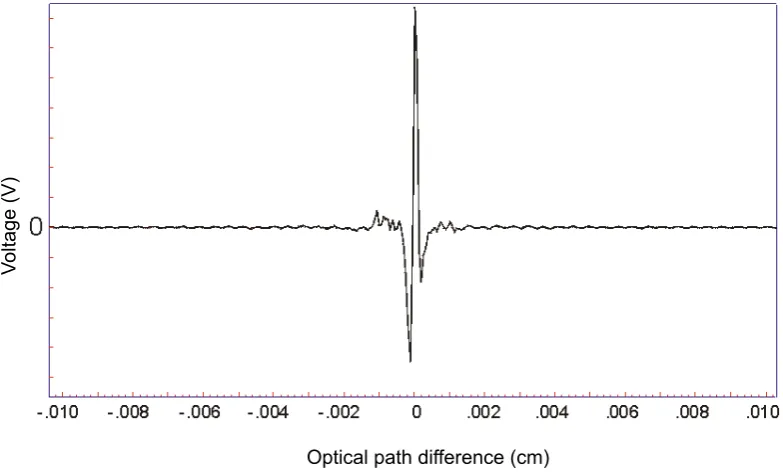
movable one. The beams reflected from the mirrors are combined and directed to the detector, where the difference of the intensities of the beams are measured as a function of the paths travelled by each beam. The measured signal is then amplified, digitized by the analog-to-digital converter and recorded. The result is a wave in time domain called an interferogram (Fig. 1.3).

Optical path difference (cm)

V

ol

ta

ge

(V)

Figure 1.3: An example interferogram from an FT-IR reading.

The interferogram contains all frequencies of IR measured in the experiment superimposed into one signal. In order to convert the time domain interferogram into a frequency domain spectrum a Fourier transform is performed on the data (Fig. 1.3). After the transformation the data is ready to be processed and analysed.

1.4.2 Data Acquisition and Analysis

data is then scaled to unit variance to prevent variables with relatively greater values being weighted heigher in the results of the analysis. The data processing results in a data set where each sample is represented by a spectrum, and each spectrum consists of numeric values corresponding to absorbances at each wavenumber. In this format data can be subject to statistical analysis. The multivariate analysis techniques often used on FT-IR (and other spectroscopic techniques) data are discussed in Section 1.7.

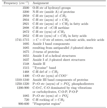
Table 1.1: Tentative assignment of bands frequently found in biological FT-IR spec-tra.

Frequency (cm−1) Assignment

3500 O-H str of hydroxyl groups 3200 N-H str (amide A) of proteins 2959 C-H str (asym) of -CH3 2934 C-H str (asym) of> CH2

2921 C-H str (asym) of> CH2 in fatty acids 2898 C-H str of→C-H methine

2872 C-H str (sym) of -CH3

2852 C-H str (sym) of> CH2 in fatty acids

1741-1715 > C =O str of esters, carbonic acids, nucleic acids 1695 Amide I band components

1685 resulting from antiparallelβ-pleated sheets 1675 β-turns of proteins

1655 Amide I ofα-helical structures 1637 Amide I ofβ-pleated sheet structures 1548 Amide II

1515 ”Tyrosine” band 1468 C-H def of> CH2

1400 C=O str (sym) ofCOO−

1310-1240 Amide III band components of proteins 1250-1220 P=O str (asym) of> P O−₂ phosphodiesters

1200-900 C-O-C, C-O dominated by ring vibrations or carbohydrates, C-O-P, P-O-P

1085 P=O str (sym) of> P O−₂ 720 C-H rocking of> CH2 900-600 ”Fingerprint region”

1.5

Nuclear Magnetic Resonance Spectroscopy

NMR spectroscopy is a powerful tool for metabolomics. It relies on elements that possess a magnetic spin number higher than zero and most of elements in organic compounds have an isotope with this property. The technique is operated in a magnetic field and uses electromagnetic radiation at radiofrequencies that allow for non-destructive data collection. It is also very robust and reproducible further adding to its value as a metabolomics tool. The one disadvantage of NMR spec-troscopy is its low sensitivity compared to techniques like mass spectrometry. The most abundant nucleus observed by NMR is1H and therefore 1D 1H NMR is the most popular among metabolomics researchers. We chose this type of NMR for this study and therefore all the following discussions of NMR spectroscopy will be describing 1D1_{H NMR experiments.}

1.5.1 Working Principles Behind NMR

Nuclear magnetic resonance is a property of the nucleus of an atom that arises from its magnetic property called spin (I). Nuclei of atoms can have a range of values of I, the most useful for NMR are nuclei withI = 1₂. This includes 1H,13C,15N,19F, 31_{P. A nuclear spin can be understood as an equivalent to a bar magnet. Placed} in a magnetic field a particle with I = 1₂ aligns itself either along or against the magnetic field entering one of two possible energy states. The nuclei in parallel with the magnetic field are in the lower energy state while the nuclei that oppose the direction of the external magnetic field are in the higher energy state. A pulse of radiofrequency can be absorbed by the nuclei in the lower energy state and be shifted to the higher energy state. This absorption or subsequent gradual release of the energy as the nuclei shift back to the lower energy state is recorded as the free induction decay (FID) and is the output of the spectrometer. In a sample each particle is affected by not just the external magnetic field but also the magnetic force exerted by the nearby particles. The effective magnetic field arising from combined magnetic influences to a nucleus determines the frequency of radiation it absorbs -its effective resonance frequency. Each observable nucleus in the sample contributes a signal to the spectrum at its resonance frequency with the area under the curve proportional to the abundance of that chemical group in the sample.

The Anatomy of an NMR Spectrometer

The NMR instrument consists of several major components:

• the probe

• radiofrequency sources

• the field frequency lock system • the shim system

• signal amplifier

• analog/digital converter (ADC) • computer

The magnet provides the external magnetic fieldB0to the sample. Nowadays it usually is a superconducting magnet, consisting of a coil submerged into liquid helium in order to reduce the electric resistance in the coil to zero. The probe is po-sitioned inside the magnet within a shim tube. It contains the receiver/transmitter coil (in some cases two coils tuned to different frequencies) that detects the signal. The radiofrequency sources produce the sine/cosine shaped waves as well as mod-ulated and shifted waves that are used to excite the nuclei during the experiment. The signal amplifiers are connected to the probe and are used to amplify the signal delivered from the probe before it reaches the ADC. The signal detected in the NMR spectrometer is analog and has to be digitised before it can be subject to Fourier transformation. The digitisation of the signal is performed by the ADC. Usually 16 - 18 bit digitizers are used which places a bound on the signal amplitude resolution at 218points. Due to this technical limitation the receiver gain of the spectrometer has to be adjusted so that the peak with the highest amplitude in the spectrum is as close to 218as possible to achieve the maximum amplitude resolution. The digitized signal is then sent to the computer where it is stored, processed and analysed.

The shim system is a system of small coils that act as adjustable magnets around the sample. Since the signal depends on the magnetic field strength a highly homogeneous magnetic field is required to collect high resolution data. Inhomogene-ity of the magnetic field in the sample would result in broadening of the peaks in the spectrum due to slightly varying frequencies of resonance of the same functional groups in different parts of the sample volume. The shimming system is used to correct such inhomogeneities in the magnetic field provided by the main coil.

lock system as a shift in the deuterium peak which prompts the system to adjust the magnetic field so the peak is shifted back to its original position consequently keeping the data signal stable.

Origin of the NMR Signal

As mentioned previously NMR spectroscopy relies on nuclear spin that gives rise to the effect of nuclear magnetic resonance. Spin is a fundamental property of elementary particles and can have values that are multiples of 1₂. Proton has a spin of 1₂ and is the most popular nucleus (we will refer to it as proton) in NMR studies. The spin can be understood through the analogy of a magnet bar that has south and north poles, or a needle of a compass and can be represented as a magnetic vector. When placed in a magnetic fieldB0 the magnetic vector aligns to the direction of the field in a parallel or anti-parallel way that corresponds to two energy levels: lower α and higher β, respectively. A proton in α state can absorb a photon of a specific energy and shift to theβ state. The energy of the photon is

E =hγB (1.1)

whereγ is the gyromagnetic ration of the particle (for hydrogen, γ = 42.58 MHz/T), B is the magnetic field strength andh is Planck’s constant (h= 6.626× 10−34J s). This energy is equal to the energy difference between theαand β states. In the experimental conditions we always speak about a group of protons in the sample as opposed to each proton separately. All the protons align parallel or anti-parallel to the external magnetic field. The populations of protons in each spin state at room temperature are not equal. The number of protons in the lower energy level (N+) is higher than the number of protons in the higher (N−). From Boltzmann statistics

N− N+ =e

−E/kT _(1.2)

where E is the energy difference between the spin energy states, k is the Boltzman constant (k= 1.3805×10−23_{J/K) and T is the temperature in Kelvin.} As the temperature increases the ratio approaches one. The signal in the NMR originates from the differences in energy absorbed and subsequently released by the spins as they transition between energy states. For this reason the signal is proportional to the difference between populations in each state.

α

β

β

β

Β

Β

Radiofrequency

Figure 1.4: Schematic illustration of the flip of magnetisation vectors of nuclear spins through application of a radiofreaquency in the NMR probe. B0 - external magnetic field,α, β - two energy states of the nuclei.

energy depends on the magnetic field strength the particle is in. In an NMR ex-periment the magnet provides the external field (B0) however this field is not expe-rienced equally by all protons. The magnetic field affecting each proton is altered by the magnetic fields created by the neighbouring nuclei. This alteration is often called the magnetic shielding and it determines the size of the effective magnetic field (Bef f) a particle is affected by. The energy required to excite a proton to

the higher energy state therefore depends onBef f rather thanB0. Subsequently in

experimental conditions the population of protons consists of subpopulations that differ in the energy required to excite the protons in that subpopulation.

In an NMR experiment the energy is provided by the electromagnetic pulse that contains a range of frequencies. The energy can be related to frequency (ν) through

E=hν (1.3)

and in an NMR experiment falls in the radiofrequency range. The differences in excitation energy (frequency) are recorded in the NMR spectrum as different peaks.

z

_z

y

y

x

x

Radiofrequency

x

x

y

y

Figure 1.5: Schematic illustration of magnetisation vector synchronisation after the application of the radiofrequency pulse. Top a view in 3 dimensions, bottom -projection onto the xy plane. The red arrows represent the -projection of the net magnetisation vector in the xy-plane that is measured by the detector.

decaying oscillation over time - the free induction decay.

1.5.2 An NMR Experiment

Data Acquisition

An NMR experiment consists of the following steps:

• preparation and insertion of the sample • setting the temperature

• locking • shimming

• acquisition parameter set-up • tuning of the probe

• calibration of the 90◦ pulse • data acquisition

Data Processing

The acquired data is in the form of a FID. It is a complex composite signal consisting of a series of oscillating signals (one for each group of nuclei with unique resonance frequency) that is detected by the receiver, amplified, digitized and recorded. In order to obtain an NMR spectrum ready for analysis from a FID there are a series of processing steps:

1. FID processing

(a) apodization

(b) zero-filling

(c) Fourier transform

2. spectrum processing

(a) phase correction

(b) baseline correction

(c) warping

(d) binning and integration

3. bin processing

(a) normalization

(b) scaling

Apodization is a transformation of the FID in order to manipulate spectral resolution and signal to noise ratio (S/N). The resolution of the spectrum depends on the speed of decay of the FID therefore the amount of signal remaining will determine the resolution (more signal at the end of the FID means more resolution). The S/N on the other hand depends on the amount of the signal at the beginning of the FID. Therefore by manipulating the FID it is possible to trade between S/N and resolution. e.g. multiplying the FID by an exponential function (exponential apodization)

W(t) =e−πlbt (1.4)

wherelbis the value of line broadening to apply, will result in improved S/N at the cost of resolution, while multiplication by a Lorentz-to-Gaussian

where lb is the line broadening factor and gb is the centre of the Gaussian emphasizes the middle and tail parts of the FID and will increase the resolution at the cost of S/N.

Zero filling is a procedure used to maximise the resolution of the spectrum obtained from the Fourier transform. It consists of adding a series of zeros after the FID equal to the number of points in the FID. After the zero-fill the Fourier transform is performed in order to transform the time domain FID into the frequency domain spectrum. The Fourier theorem states that every periodic function can be decomposed into a series of sine and cosine functions with different frequencies and is defined as

f(ω) =

Z ∞

−∞

f(t)e−iωtdt=

Z ∞

−∞

f(t)[cos(ωt)−isin(ωt)]dt (1.6)

whereωis the frequency andtis time. In practice the FID is discrete and the Fourier transformation is performed using the Cooley-Tukey fast Fourier transform (FFT) algorithm [Cooley and Tukey, 1965] which converts a discrete time-seriesxk

of length N into a spectrum with N points:

f[n] = √1 N

N−1 X

k=0

xke−2πkn/N (1.7)

It has a constraint that the number of points in the FID has to be a power of 2. Therefore the number of points collected in a FID is usually 16384, 32764, 65536, etc.

as flat as possible. This is not always achieved by default and baseline correction is required in the processing phase. A variety of methods for baseline correction of NMR spectra have been proposed [Bartels et al., 1995; Brown, 1995; Golotvin and Williams, 2000; Xi and Rocke, 2008]. The methods are based on fitting func-tions to the baseline and subtracting the fitted values from the spectrum to flatten the baseline. Another frequent problem in preparation of NMR data for analysis especially in metabolomics studies is peak shifts due to pH and ionic strength vari-ation between samples. This makes data comparison, especially using automated methods, harder. There have been a series of algorithms proposed for automatic alignment (warping) of NMR spectra [Forshed et al., 2003; Lee and Woodruff, 2004; Veselkov et al., 2009]. The algorithms are usually based on dividing the spectra into segments and using an optimization algorithm to shift the segments until the optimal alignment is achieved.

In metabolomic studies, after the spectrum is processed it is reduced in di-mensionality through binning and integration under the curve. Since the spectra acquired in the NMR experiments often contain more than 30,000 data points it is not efficient to perform statistical analysis on such a high-dimensional dataset. Therefore the spectra are divided into segments and for each segment the area under the curve is computed. The most popular methods of binning are “uniform”, when binning is performed in intervals of a constant preset length (e.g. 0.05 ppm), and “adaptive”, when the intervals are of variable length and each spans a peak or a group of peaks. The latter can be performed manually by creating a bin table that is used for the whole experiment or through the use of an automated algorithm [Keun et al., 2003; Davis et al., 2007; Worley and Powers, 2015].

A binned dataset is then subject to normalization and scaling. Normalization is a process of transformation of data to account for differences between samples (e.g. dilution factors) making them comparable to each other. In such a case the spectra can be normalized either by the area of a peak that is invariant between samples, the reference peak or the total integral of the spectrum [Craig et al., 2006]. Data scaling on the other hand is performed on each variable (in this case each bin) across the dataset. It makes the variables more comparable and avoids unwanted weighting of the data without biological content contributing to the results and suggesting errorneus conclusions [van den Berg et al., 2006].

yields the best results for each specific case.

1.6

High Content Imaging

1.6.1 HCI Experiments and Data Collection

The three key components in an HCI experiment are cells bound with a fluorophore in order to visualize appropriate cellular components, an image collection platform and image analysis algorithms. The fluorophores can roughly be classified into three categories: autofluorescing proteins that are engineered into the cells [Talman et al., 2010], fluorescent dyes that enter the cells and concentrate in a particular compartment or bind intracellular components such as SYBR Green [Zipper et al., 2004] or Hoetch [Latt et al., 1975], and antibodies with affinity to the desired target that are directly tagged with a fluorescent molecule. The fluorescent tag helps to visualize the target component of the cell.

The image collection platform usually consists of a fluorescence microscope, a dynamic system for positioning the cell culture plate under the microscope, a high resolution camera system for capturing the images and a mechanism for data storage [Gough and Johnston, 2006]. The system is usually equipped with a set of excitation and emission filters to allow for selection of wavelengths during image capture. This allows multiple probes to be used in the same sample without much interference. Some systems (Opera, Perkin Elmer) come with multiple digital cameras that allow simultaneous multichannel image capture. Simultaneous image capture is quicker than the sequential method however it requires careful selection of fluorescent probes to avoid wavelength overlap [Lee and Howell, 2006].

Software plays a very important part in the high content imaging pipeline. The first part is the software that controls the imaging system. It is used to set the parameters for the experimental procedure. It collects the images and stores them in a database system, reports faults and performs quality control. The second part of the software in the pipeline is the data analysis software. The analysis software is used for data visualization and data processing which includes artefact detection, selection of the fluorescent signal fields and measurement of a variety of parameters including size, intensity, various shape and texture parameters, and behaviour over time. The user defines the analysis parameters and the images are automatically processed. Once the assay is tested and validated the system can run mostly automatically allowing for robust high throughput data collection [Berlage, 2005; Pepperkok and Ellenberg, 2006].

1.7

Statistical Data Analysis

regions the data consists of multiple measurements per sample and often the num-ber of variables (measurements) exceeds the numnum-ber of samples. Such cases demand multivariate techniques for analysis - data explorations and hypothesis generation, pattern detection or hypothesis testing. Here we briefly introduce the statistical techniques used in this work. We discuss some mathematical definitions, the intu-ition behind the methods and result interpretation as well as suitable applications and their merits.

1.7.1 Principal Component Analysis

Principal component analysis (PCA) is a linear data transformation that yields a set of latent (unobserved) variables, usually referred to as principal components (PC). Principal components are linear combinations of raw variables such that the first principal component contains the most variation from the original data. The subsequent principal components are selected to be orthogonal to the first one and contain maximum variance unaccounted by preceding PCs. This procedure creates a new data set where each variable is substituted by a PC however only a small number of PCs is required to account for the majority of the variance in the original data. As only a small amount of variance is accounted for by a large set of PCs they can be ignored without losing much information, effectively reducing the data set to a smaller number of variables. PCA is often referred to as a dimensionality reduction technique as the reduction of number of variables can be seen as project-ing the data to a lower-dimensional space. PCA is usually performed in order to reduce the dimensionality of the data for easier visualization or more robust mod-elling. Plotting the first two or three principal components as a scatterplot is often used as an exploratory method to get insight into the structure in the data. For ex-ample clustering of data points (each point represents a sex-ample) might be observed suggesting similarities between treatment effects if points cluster together (andvice versa). PCA is often used to reduce the number of variables before applying a

pre-dictive modelling technique as the smaller number of variables often lead to simpler and subsequently more robust models.

PCA is usually performed in one of two ways: either through Eigen decompo-sition of the covariance matrix of the data or through singular value decompodecompo-sition (SVD). The latter method is more numerically stable and therefore is preferred in most cases. SVD decomposes a mean-centered (each column has its mean subtracted from it)m×n matrixX into three parts:

where U is an m×m matrix containing the left singular vectors, D is an a×adiagonal matrix containing the singular values andVis an×amatrix of right singular vectors. The product UD constitutes the so called PCA scores matrix. The scores matrix is the transformed data obtained from the PCA and used for visualization of further analysis. TheVmatrix is the loadings matrix whose columns contain the weights of the original variables in each PC. They can be investigated in order to determine variable contribution to each PC. The diagonal matrix D

contains values whose squares are proportional to the variances accounted for by each corresponding PC

λi=d2i/(n−1) (1.9)

where λ is the variance of the i-th component and the fraction of variance accounted for by each PC can be calculated from

F(i) =λi/ a

X

j=1

λj (1.10)

The fraction of the variance accounted for by each PC can be used to assess the information provided by keeping each principal component. Often the first few principal components account for the majority of the variance and the structure in the data can be adequately visualized by plotting the PCs.

1.7.2 Linear Discriminant Analysis of Principal Components

Linear discriminant analysis (LDA) is a classification technique that transforms the data into a different space where the discrimination between groups in data is maximised while within group differences are minimised. It is similar to PCA in that the data is linearly transformed into a different space, however while PCA aims to find the directions of maximum variance in the data as a whole, LDA finds the directions of maximum separation between groups. LDA is therefore performed on data that has grouping labels (e.g. sample treatment groups) and is often used as a technique to show differences between treatments. The resulting model can also be used to assign new data samples to groups in the data that model was built on (this procedure is usually referred to as model training). Formally the LDA finds the linear combination of variablesa that maximises the ratio of the sum of square differences between groupsB and the sum of square differences within groupsW:

whereW and B are calculated as

W=

G

X

i=1

˜

XT_i X˜i (1.12)

B=

G

X

i=1

ni(¯xi−¯x)(¯xi−¯x)T (1.13)

whereGis the number of groups, X˜i is the mean-centered data matrix only

containing objects of group i, ¯xi is the mean vector for the group i and x¯ is the

mean vector for the whole data. TheW is the variation within each group (around group centre) andB is the variation of the group centres around the global mean. The solutionais found by maximising Equation 1.11.

As the number of variables in the data increases the LDA model becomes less robust and requires more data. In cases when the data is high-dimensional it is often beneficial to reduce the dimensionality of the data before performing LDA. PCA is a frequently used method for this purpose. The technique is then referred to as LDA-PC or DA-PC. In order to build a robust LDA-PC model and avoid fitting to the noise in the data (overfitting) the number of PCs to be used for LDA has to be determined. A popular way of model selection is cross-validation. It consists of splitting the data into subsets and training the model on the data leaving one subset out so called Nfold crossvalidation, where N is the number of partitions -and using that partition to test the model. A robust model will perform similarly on each of the partitions. Such a cross-validated scheme of model building can be then used on data consisting of increasing number of principal components and each time a model fit metric e.g. Q2 can be used to assess the model. The best average metric value will determine the optimal number of PCs to use.

1.7.3 Partial Least Squares Discriminant Analysis

T=XW (1.14)

such that covariance betweenY andTis maximised. Ordinary least squares procedures are used to regressYonTin order to compute a weights matrixQsuch that

Y=TQ+E (1.15)

whereE is an error matrix. The model is then defined as

Y =XB+E (1.16)

B=WQ (1.17)

The model is usually computed using the NIPALS algorithm [Geladi and Kowalski, 1986]. While PLS regression is used to predict response variables PLS-DA is used to predict classes of the observations. It is done by using “dummy” variables to form a binary n×p matrix Y where n is the number of observations andp is the number of groups minus one such thatYij = 1 if observationibelongs

to classjand otherwise Yij = 0. This matrix is then used in the PLS algorithm as

the response matrix. In order to avoid model over-fitting an appropriate number of components to be used in the model has to be selected. For this purpose the same cross-validation procedure as in Section 1.7.2 can be used.

1.7.4 Permutation Test