University of Warwick institutional repository: http://go.warwick.ac.uk/wrap
A Thesis Submitted for the Degree of PhD at the University of Warwick
http://go.warwick.ac.uk/wrap/62064
This thesis is made available online and is protected by original copyright.
Please scroll down to view the document itself.
via SEQUENTIAL MONTE CARLO
by
Yan Zhou
A thesis submitted to the University of Warwick in partial fulfillment of the requirements for the degree of
Doctor of Philosophy
The University of Warwick
Department of Statistics
list of tables vi
list of figures vii
acknowledgements 1
declarations 2
abstract 3
1 introduction 4
1.1 Context 5
1.2 Notations 6
1.3 Outline 7
2 positron emission tomography compartmental model 9
2.1 Compartmental model 9
2.2 Application to positron emission tomography 10 2.3 Simulated and real pet data 15
2.4 Modeling error structures 17
3 model selection 19
3.1 Information-theoretic approach 19 3.1.1 Kullback-Leibler divergence 19 3.1.2 Akaike’s information criterion 21 3.1.3 A second order aic 23
3.2 Bayesian model comparison 29 3.2.1 Model choice problems 29
3.2.2 Bayes factor 32
3.2.3 Choice of priors 36
3.3 Discussions 44
4 monte carlo methods 47
4.1 Classical Monte Carlo 47
4.2 Importance sampling 49
4.3 Markov chain Monte Carlo 51
4.3.1 Discrete time Markov chain 52 4.3.2 Metropolis-Hastings algorithm 54
4.3.3 Gibbs sampling 62
4.3.4 Reversible jump mcmc 67
4.3.5 Population mcmc 69
4.3.6 Convergence diagnostic 74
4.3.7 Application to Bayesian model comparison 79
4.4 Discussions 84
5 sequential monte carlo for bayesian computation 85
5.1 Sequential Monte Carlo samplers 86
5.1.1 Sequential importance sampling and resampling 86
5.1.2 smc samplers 90
5.1.3 Sequence of distributions 91 5.1.4 Sequence of transition kernels 93
5.1.5 Optimal and suboptimal backward kernels 94 5.2 Application to Bayesian model comparison 96
5.2.1 smc1: An all-in-one approach 96
5.2.2 smc2: A direct-evidence-calculation approach 98 5.2.3 smc3: A relative-evidence-calculation approach 100 5.2.4 Path sampling via smc2/smc3 101
5.3 Extensions and refinements 103
5.4 Theoretical considerations 118 5.5 Performance comparison 119
5.5.1 Gaussian mixture model 120
5.5.2 Nonlinear ordinary differential equations 126
5.5.3 pet compartmental model 133
5.5.4 Summary 142
5.6 Discussions 143
6 vsmc: a c++ library for parallel smc 145
6.1 Background 146
6.1.1 Parallel computing 146
6.1.2 Software for Monte Carlo computing 151
6.2 ThevSMClibrary 156
6.2.1 Core classes 157
6.2.2 Program structure 159 6.3 The particle system 162
6.3.1 A matrix of state values 162 6.3.2 A single particle 163
6.3.3 Example: The value collection of gmm 164 6.4 Initializing 168
6.4.1 Example: Simulation of a Normal distribution 168 6.4.2 Parallelized implementation 169
6.5 Updating 173
6.5.1 Example: Updating the weights in the smc2 algorithm 173
6.5.2 Example: The mcmc move in gmm 175
6.6 Monitoring 178
6.6.1 Example: Path sampling in the smc2 algorithm 180 6.6.2 Example: Adaptive specification of proposal scales 180
6.7 Performance 184
6.7.1 Using the smp module 185 6.7.2 Using theOpenCLmodule 185 6.7.3 Performance and productivity 188
6.8 Discussions 190
7 conclusions 192
7.2 Future directions 193
references 195
a monte carlo methods 211
a.1 Discrete time Markov chain 211 a.1.1 Irreducibility 211
a.1.2 Cycles and aperiodicity 212
a.1.3 Recurrence 213
a.1.4 Invariant measure 213
a.1.5 Ergodicity 214
b sequential monte carlo for bayesian computation 216
b.1 Proof of proposition 5.1 216
c vsmc: a c++ library for parallel smc 222
c.1 Classes of parallel computers 222 c.1.1 Instruction level 222
c.1.2 Multicore processors and symmetric multiprocessing 222
c.1.3 Distributed computing 223 c.1.4 Massive parallel computing 223 c.2 Parallel patterns 224
c.2.1 Map 224
c.2.2 Fork-join 225
c.2.3 Reduction 225
c.2.4 Pipeline 226
c.3 Modern C++ 226
c.3.1 Templates 227
3.1 Model selection results for the pet compartmental model using the aic𝑐strategy 24
3.2 Jeffreys’ intepretation of the Bayes factor 33
3.3 Model selection results for the pet compartmental model using the bic strategy 35
3.4 Model selection results for the pet compartmental model using the Bayes factor (vague priors) 40
3.5 Model selection results for the pet compartmental model using the Bayes factor (informative priors) 43
5.1 The standard Bayes factor estimates for a simulated pet data set using adaptive and non-adaptive smc algorithms 117
5.2 The number of distributions used for a simulated pet data set using adaptive and non-adaptive smc algorithms 118
5.3 Gaussian mixture model posterior model probability estimates 123 5.4 Gaussian mixture model the Bayes factor estimates 123
5.5 Nonlinear ode model marginal likelihood and the Bayes factor estimates (simple model data) 129
5.6 Model selection results of nonlinear ode model using the Bayes factor (simple model data) 130
5.7 Nonlinear ode model marginal likelihood and the Bayes factor estimates (complex model data) 131
5.8 Model selection results of nonlinear ode model using the Bayes factor (complex model data) 132
5.9 pet compartmental model marginal likelihood estimates 136 5.10 pet compartmental model the Bayes factor estimates 137 5.11 Path sampling marginal likelihood estimates bias reduction for a
2.1 Illustration of the plasma input pet compartmental model 12 2.2 Illustration of the three-compartments plasma input pet model. 15
4.1 Traces of parameters in the random walk algorithm for the pet compartmental model (calibrated) 59
4.2 Traces of parameters in the random walk algorithm for the pet compartmental model (uncalibrated) 60
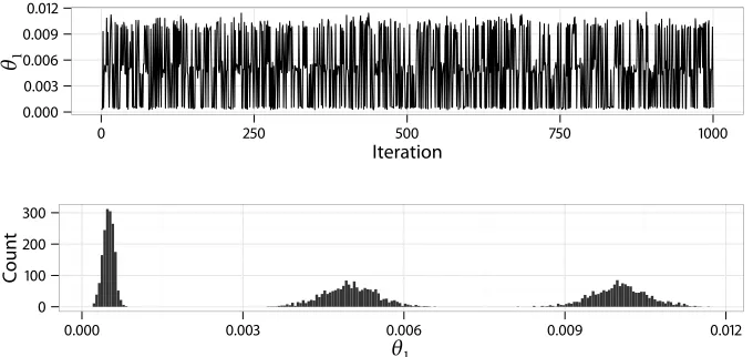
4.3 Trace and histogram of parameters in the random walk algorithm for the pet compartmental model (calibrated) 75
4.4 Trace and histogram of parameters in the random walk algorithm for the pet compartmental model (uncalibrated) 76
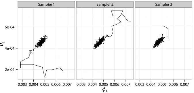
4.5 Convergence diagnostics for the random walk algorithm for the pet compartmental model using summary statistics 77
4.6 Convergence diagnostics for the random walk algorithm for the pet compartmental model using averages 78
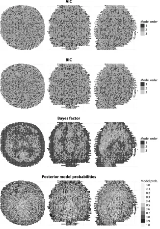
4.7 Model selection results for the pet compartmental model 83
5.1 Typical real pet data 105
5.2 Variations of the distribution specification parameter for the pet compartmental model using adaptive smc algorithms 109
5.3 Relationship between average number of distributions and cess 111 5.4 Relationship between the variance of the path sampling estimator and
cess 112
5.5 Acceptance rates of adaptive smc algorithms 114 5.6 Acceptance rates of non-adaptive smc algorithms 115
5.7 Variance of standard standard estimator and path sampling using adaptive resampling 124
5.8 Volume of distribution estimates of real pet compartmental model
data 134
5.9 Variance of path sampling estimator and total number of samples using smc algorithm 140
First and foremost, I would like to sincerely express my deepest gratitude to my supervisors John Aston and Adam Johansen for their enthusiasm, encouragement and for introducing me to such exciting topics. The discussions and feedback during the course of this thesis were immensely appreciated. I am also grateful to them both for their trust in allowing me the freedom to follow my ideas and develop side projects.
No words can express my gratitude to my parents for all their support. Indeed this thesis would have never been possible without their constant encouragement.
To Zhou Yongjun & Han Ping
This thesis is submitted to the University of Warwick in support of my application for the degree of Doctor of Philosophy. It has been composed by myself and has not been submitted in any previous application for any degree excepting some of the background material in Chapter 2, which was based on a dissertation previously submitted to the University of Warwick for the degree of Master of Science. This declaration confirms that this thesis is original and sole work of the author alone. Parts of this thesis have been published by the author:
Y. Zhou.vSMC: Parallel sequential Monte Carlo in C++. Mathematics e-print 1306.5583. ArXiv, 2013
Y. Zhou, A. M Johansen, and J. A. Aston.Towards automatic model
compari-son: an adaptive sequential Monte Carlo approach. Mathematics e-print 1303.3123.
ArXiv, 2013
Y. Zhou, J. A. D. Aston, and A. M. Johansen. “Bayesian model comparison for compartmental models with applications in positron emission tomography”.
Journal of Applied Statistics40.5 (2013), pp. 993–1016
Yan Zhou, Adam M. Johansen, and John A. D. Aston. “Bayesian model selec-tion via path-sampling sequential Monte Carlo”. In:Proceedings of IEEE Statistical
Signal Processing Workshop. 2012
The sequential Monte Carlo (smc) methods have been widely used for modern scientific computation. Bayesian model comparison has been successfully applied in many fields. Yet there have been few researches on the use of smc for the purpose of Bayesian model comparison. This thesis studies different smc strategies for Bayesian model computation. In addition, various extensions and refinements of existing smc practices are proposed in this thesis. Through empirical examples, it will be shown that the smc strategies can be applied for many realistic applications which might be difficult for Markov chain Monte Carlo (mcmc) algorithms. The extensions and refinements lead to an automatic and adaptive strategy. This strategy is able to produce accurate estimates of the Bayes factor with minimal manual tuning of algorithms.
This thesis studies the use of sequential Monte Carlo (smc) algorithms for the pur-pose of Bayesian model comparison. The main focus of the work is the performance of the Monte Carlo algorithms when they are used in the context of Bayesian model comparison. Contemporary methodologies on model selections and Monte Carlo methods for the purpose of Bayesian model comparison are reviewed. Method-ologies on using smc in this context are developed. Some extensions to as well as refinements of existing smc practices are also presented in this work.
The performance of smc algorithms for the purpose of Bayesian model com-parison is studied empirically through various realistic models. Some theoretical results are also derived for non-standard methods. As this thesis covers a wide array of topics, one particular model, the position emission tomography (pet) compart-mental model, is used as a running example for illustrating purpose throughout this thesis. This model is introduced in the next chapter. However, it shall be noted that, this thesis is not concerned with the analysis of the pet data in general. The particular model used in this thesis is chosen for a few reason. It provides a gen-uine model selection problem to which different methods can be applied and their performance can be compared. In the context of Bayesian model comparison, it is also considerably computationally challenging, in the sense that many widely used Monte Carlo methods might not perform well for practical use. The smc algorithms are very well suited for this and many other realistic Bayesian model comparison problems. And the advantage of the smc algorithm can be made more clear through such and other realistic models.
1.1 context
Model comparison and selection are problems found throughout the discipline of statistics. It can appear in different forms, such as the choice of regressors in regression analysis, or the determination of the number of components in mixture models. Often, there can be more than one model that can be potentially used to describe the data and to make predictions or for other purposes. However, some models might be better than others in the sense that the estimation and prediction based on them have smaller errors or variances, etc. Some models are simpler than others while providing comparable accuracy. In many application areas, model selection is also important for the purpose of identifying the underlying reasons of certain phenomena observed through the data. Many model selection and comparison methods have been developed throughout the history of statistics. Some of them are developed for particular classes of models while others make little assumptions of the candidate models. This thesis is more concerned with the later.
Bayesian model comparison has been studied and practiced for a long time. There are considerable computational difficulties when using this approach, as many high dimensional integrations are involved. The development of Monte Carlo algorithms has enabled the practice of Bayesian model comparison for a wide range of realistic applications. However, algorithms such as Markov chain Monte Carlo (mcmc) cannot efficiently simulate high dimensional multimodal distributions in many situations. In addition, estimators of quantities for the purpose of Bayesian model comparison, such as the Bayes factor, obtained through these algorithms are often unreliable in the sense that with manageable computational cost, the variances are often too large for practical use. In some cases, reliable and efficient estimators can be obtained, but they are often less generic as they require knowledge of the models not generally available. In this thesis, we aim to develop high performance algorithms that are both generic and reliable.
dimen-sional multimodal distributions. Reliable estimators of quantities such as the Bayes factor can also be obtained through these algorithms. However, there is little literature on its application to Bayesian model comparison. This thesis presents a framework based on sequential Monte Carlo (smc) algorithms, within which Bayesian model comparison can be carried out in a (semi-) automatic fashion while better accuracy compared to some other recent developments can be obtained. This is made possible through the use of various adaptive strategies.
This thesis also presents work on the practical implementations of smc algo-rithms. Compared to mcmc, practical tools for smc are relatively fewer. In addition, there is interest in the utilization of parallel computing for the implementation of smc algorithms. The work presented in this thesis provides a toolbox with which re-searchers can implement generic smc algorithms on parallel computers with relative ease.
1.2 notations
Most notations used in this thesis are introduced and defined in context. A few conventions are followed throughout this thesis.
Capital Latin letters, such as𝑋, are used to denote random variables and corresponding lower case letters, such as𝑥, are used to denote their realizations. In the context of Markov chain, we use notations such as𝑋𝑡to denote the random variable to indicate its dependency on time𝑡. For various Monte Carlo estimators, we use notations such as𝑋(𝑖)to denote the random samples, including the case of mcmc algorithms. The difference between𝑋𝑡and𝑋(𝑖)is to explicitly express that in some algorithms, not all samples from a Markov chain are used for estimation purpose. For smc algorithms, we use𝑋(𝑖)𝑡 to denote the particle value of the𝑖th particle at time𝑡. For a sequence of variables, such as𝑋1, … , 𝑋𝑛, we use the notation 𝑋1∶𝑛to denote the sequence.
is used to denote the expectation with respect to a distribution𝜋. The lettersPrare used to denote probabilities of random events.
For a scalar function of an𝑛-vector𝜃 = (𝜃1, … , 𝜃𝑛)𝑇, say𝑓(𝜃), we use the notation, 𝜕2𝑓(𝜃)
𝜕𝜃𝜕𝜃𝑇 to denote the Hessian matrix, i.e., a matrix whose element at the 𝑖th row and𝑗th column is𝜕𝑓(𝜃)/𝜕𝜃𝑖𝜃𝑗. We also use the notation 𝜕𝑓(𝜃)
𝜕𝜃 to denote the score vector whose𝑖th element is𝜕𝑓(𝜃)/𝜕𝜃𝑖. For an𝑚-vector function𝑓(𝜃) = (𝑓1(𝜃), … , 𝑓𝑚(𝜃)), we use the notation𝐽(𝑓(𝜃)) = 𝜕𝑓(𝜃)
𝜕𝜃 to denote the Jacobian matrix whose element at the𝑖th row and𝑗th column is𝜕𝑓𝑖(𝜃)/𝜕𝜃𝑗.
To avoid introducing too many notations, some notations might be reused if their meanings are clear in the context and their usage is limited to a particular section where they are relevant. These and other notations are defined when they are encountered the first time.
1.3 outline
This thesis is concerned with the methodologies of using smc algorithms for the purpose of Bayesian model comparison and their practical implementations. It is structured as the following.
Chapter 2 introduces the positron emission tomography (pet) compartmen-tal model. It is a realistic model that will be used as a running example throughout this thesis to demonstrate various methodologies. Work on the application of Bayesian model comparison to the pet compartmental model was published in [167].
Chapter 3 reviews some commonly used model selection methods. In partic-ular some information-theoretic selection criteria and the Bayesian approach. By comparison, it will be shown that Bayesian model comparison is of interest for some realistic applications where its use was previously limited by the computational cost.
Chapter 4 reviews some Monte Carlo algorithms in the context of Bayesian
for many problems of interest.
Chapter 5 presents a framework based on smc that can be used for the
pur-pose of Bayesian model comparison. In particular, various adaptive strategies will be discussed. This chapter is an extension to [168] and [169].
Bayesian model comparison for the positron emission tomography (pet) com-partmental model was studied before by the author. This thesis uses this realistic example for demonstration in Chapters 3 to 5. This chapter introduces the compart-mental model and its application to pet. Later we will frequently refer to materials here for details of the model setting. This chapter is based on [167] by the author.
It shall be noted that, the application of Bayesian model comparison to the pet compartmental model is introduced here in a separate chapter only because it is used throughout the thesis as a demonstrating example. It is not unique to any of the following chapters. This thesis is not about the analysis of pet data or the compartmental model in general. Since this model is used for illustrating purpose only, only where demonstration and comparison of methods are appropriate it is used. Not all model selection and Monte Carlo methods reviewed in the next two chapters are applied to this model.
2.1 compartmental model
Compartmental models are a class of models that describe systems in which some real or abstract quantity flows between different (physical or conceptual) com-partments, each with its own characteristics. It is often of interest to infer both parameters that describe the dynamics of the system and the number of compart-ments that are required in order to adequately describe measured data within this framework. The choice of the number of compartments in the model presents a model selection problem of interest.
well-mixed material. The compartments interact by material flowing from one compartment to another. There may be flows into one or more compartments from outside the system (inflows) and there may be flows from one or more compart-ments out of the system (outflows) [81]. In this thesis, linear compartmental models are considered. In these models, the rate of tracer flow from a compartment is proportional to the quantity of tracer in that compartment. In such models the flow may be parameterized by a pair of transfer coefficients, which are termedrate
constantsand may take the value zero, for each pair of compartments.
This class of models yields a set of ordinary differential equations (ode) that describes the flow of tracer. Consider an𝑟-compartments model. Let𝑓(𝑡)be the 𝑟-vector whose𝑖th element corresponds to the concentration in the𝑖th compartment at time𝑡. Let 𝑏(𝑡)be the 𝑟-vector that describes all flow into the system from outside. The𝑖th element of𝑏(𝑡)is the rate of inflow into the𝑖th compartment from the environment. The dynamics of such a model may be written as,
̇
𝑓(𝑡) = 𝐴𝑓(𝑡) +𝑏(𝑡),
𝑓(0) =𝜉,
where𝜉is the𝑟-vector of initial concentrations and𝑓̇denotes the time derivative of𝑓. The matrix𝐴is formed from the rate constants (see [67]). The solution [142, sec. 8.3.1] to this set of equations is,
𝑓(𝑡) = 𝑒𝐴𝑡𝜉+ ∫𝑡 0
𝑒𝐴(𝑡−𝑠)𝑏(𝑠) d 𝑠,
where the matrix exponential𝑒𝐴𝑡= ∑∞𝑘=0(𝐴𝑡)𝑘!𝑘.
2.2 application to positron emission tomography
available to neuroscientists to study biochemical processes within living brains, as methodology such as magnetic resonance imaging (mri) is primarily only able to study effects via blood flow changes, while pet can study changes in the biochemical systems themselves. This is of considerable interest within research into diseases where biochemical changes are known to be responsible for symptomatic changes, such as in schizophrenia and other psychiatric diseases [47]. In a clinical setting, pet is now one of the most commonly used diagnostic procedures for cancer (both within and outside the brain), as fluoro-deoxyglucose ([18F]-FDG, an radiotracer analogue of glucose) can be imaged. Cancer cells tend to be very metabolically active, thus requiring more glucose than surrounding cells, resulting in a greater uptake of [18F]-FDG, leading to an indication of cancer location on an [18F]-FDG scan [49].
In a typical molecular assay, usually a positron-labelled tracer is injected intravenously and the pet camera scans a record of positron emission as the tracer decays [127]. With all events detected by the pet camera, the time course of the tissue concentrations are reconstructed as three-dimension images [98]. The digital image so captured shows the signal integrated over small volume elements, termed
voxels. Each voxel has a volume of the order of a few cubic millimeters. This data
provides the tissue time-activity function, which is the total concentration of tracer in all tissue compartments. In theplasma input compartmental model, in addition to the pet data, a separate measurement of the concentration of tracer in the plasma is available. This measurement is generally assumed to be noise free (it can be measured with much greater accuracy than the signal of interest). This model is used in the current study. See [67] for the pet compartmental model in general.
𝐶𝑃 𝐶𝑇 𝐶𝑇1
𝐶𝑇𝑖
𝐶𝑇𝑗
𝐶𝑇𝑟 𝐾1
𝑘2
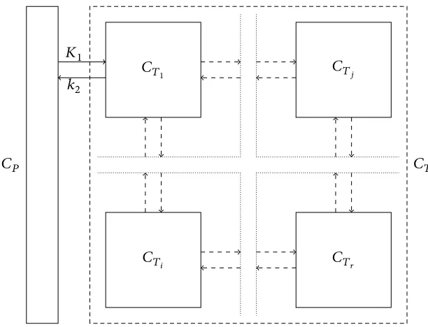
Figure 2.1 Illustration of the plasma input pet compartmental model.
the parameters of more general non-linear ode systems robustly will be close to impossible in this setting. Furthermore, on a voxel level, which is the type of spatial analysis that is of interest here, the signal-to-noise ratio of the data is not high, making any parameter estimation difficult. Finally, as the models are estimated for every voxel in the brain (typically around a quarter of a million voxels per scan), computational consideration needs to be taken into account. Thus, linear ode mod-els are both experimentally useful and computationally efficient; and it is difficult to justify the additional complexity that would arise from considering more general models.
The model used in this thesis, the plasma input model as illustrated in Fig-ure 2.1, with𝑟tissue compartments can be written as a set of ode,
̇
𝐶𝑇(𝑡) = 𝐴𝐶𝑇(𝑡) +𝑏𝐶𝑃(𝑡)
𝐶𝑇(𝑡) =1𝑇𝐶𝑇(𝑡)
[image:21.612.137.443.68.302.2]where𝐶𝑇(𝑡)is an𝑟-vector of time-activity functions of each tissue compartment, 𝐶𝑃(𝑡)is the plasma time-activity function, i.e., the input function. 𝐴is the𝑟 × 𝑟 state transition matrix with𝐴(𝑖, 𝑗)being the rate constant of tracer flowing from the 𝑖th compartment into the𝑗th compartment.𝑏= (𝐾1, 0, … , 0)𝑇is an𝑟-vector, where 𝐾1is the rate constant of input from the plasma into tissues. The𝑟-vectors1and 0correspond to the𝑟-vectors of ones and zeros, respectively. The matrix𝐴takes the form of a diagonally dominant matrix with non-positive diagonal elements and non-negative off-diagonal elements. Furthermore,𝐴is negative semidefinite [67]. The solution to this set of ode is,
𝐶𝑇(𝑡) = 𝐶𝑃(𝑡) ⊗ 𝐻𝑇𝑃(𝑡) = ∫𝑡 0
𝐶𝑃(𝑡 − 𝑠)𝐻𝑇𝑃(𝑠) d 𝑠 (2.1)
𝐻𝑇𝑃(𝑡) = 𝑟 ∑ 𝑖=1
𝜙𝑖𝑒−𝜃𝑖𝑡, (2.2)
where⊗is the convolution operator and the𝜙1∶𝑟and𝜃1∶𝑟parameters are functions of the rate constants. There is a one-to-one mapping between the set of rate constants and the set of𝜙1∶𝑟and𝜃1∶𝑟parameters (see [67] for the explicit form of the mappings for various model configurations, including the ones later used in this thesis). The input function𝐶𝑃(𝑡)is assumed to be nearly continuously measured. The tissue time-activity function𝐶𝑇(𝑡)is measured discretely, leading to measured values of the integral of the signal over each of𝑛consecutive, non-overlapping time intervals ending at time points𝑡1, … , 𝑡𝑛. The macro parameter of interest is thevolume of distribution,𝑉𝐷, defined by
𝑉𝐷= ∫∞ 0
𝐻𝑇𝑃(𝑡) d 𝑡 = 𝑟 ∑ 𝑖=1
𝜙𝑖
𝜃𝑖. (2.3)
This corresponds to the steady state ratio of tissue concentration to plasma concen-tration in a constant plasma concenconcen-tration regime. That is, if an injection of tracers into the plasma was made such that the plasma concentration remained constant over time, then the ratio of concentration in the tissues to the concentration in the plasma after an infinite time had passed would be exactly𝑉𝐷.
number of compartments can be associated with each one. The model selection problem is to find the number of compartments given the data at each voxel. The compartments in the model typically can be identified with free tracer, specifically bound tracer (tracer bound to the system under investigation) and non-specifically bound tracer (tracer bound to different competing systems), indicating the role of certain chemicals within particular brain systems. In the model fitting, a “massive univariate” approach is taken with each voxel being analyzed separately. Spatial effects are neglected in this approach and voxels are assumed to be independent. This approach is common in the literature and makes the problem of dealing with a very large number of voxels feasible. However, it imposes very stringent com-putational requirements. About a quarter of a million voxels must be analyzed (i.e., the time series analysis must be repeated separately for each of these voxels), meaning that robustness is essential as complex model-specific characterizations and model/algorithm tuning cannot be performed on a voxel by voxel basis.
The changes of the biochemical systems are reflected in the different rates of the decay of the concentration of the compounds labelled with position emit-ting radionuclides. The compartments in the context of the pet compartmental model are conceptual instead of physical. In the situation where the tracers are not interacting with the brain tissues in any way, all tracers are free tracers. They are input into the brain and flows outside it without being bound to any tissues. And thus there will be only one compartment. When the biochemical process of interest does occur within the brain, some tracers will be bound to the tissues instead of flowing outside the brain. In this case, a second compartment may be observed. It is also possible that the tracers are bound to the brain tissues but not through the biochemical process of interest. In this case, a third compartment may be observed, too.
𝐾1
𝑘2
𝑘3
𝑘4
𝑘5 𝑘6
Plasma
Non-specifically bound
[image:24.612.137.456.80.238.2]Specifically bound Three compartments
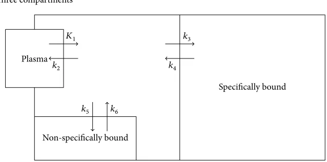
Figure 2.2 Illustration of the three-compartments plasma input pet model.
of interest is indeed happening within the brain. And thus further diagnoses through other techniques can be used to determine the cause the symptomatic changes.
2.3 simulated and real pet data
Two kinds of data are used in this thesis. The first is simulated from a three-compartments model as illustrated in Figure 2.2, with the matrix of rate constants,
𝐴 =[[[[
[
−𝑘2− 𝑘3− 𝑘5 𝑘4 𝑘6
𝑘3 −𝑘4 0
𝑘5 0 −𝑘6 ] ] ] ]
]
, (2.4)
time activities divided by the length of time frames (i.e.,𝐶𝑇(𝑡𝑖)/(𝑡𝑖− 𝑡𝑖−1)). The noise is scaled such that the highest variance in the sequence is equal to a “noise level” variable (with the others scaled in proportion). This noise level ranges from 0.01to5.12, from lower than typical region of interest (roi) analysis (in which the data is averaged over a biologically meaningful region in order to improve signal to noise ratio) to higher than the noise associated with voxel-level analysis [125]. For each noise level, 2,000 time series were simulated.
analyzed. Figure 5.1 shows the estimates of𝑉𝐷for this data obtained in a previous study [167]. It can be seen that the spatial structure of the data is heterogeneous. Ro-bustness of algorithms is needed to obtain good performance for the large number of data sets.
2.4 modeling error structures
In the scenarios considered in this thesis, linear one-, two-, and three-compartment models are considered possible; the methods could deal with other compartmental models straightforwardly, but we focus on these as they are the most interesting in the application of interest. Let𝑡1, … , 𝑡𝑛be the end points of the time frames at which the tissue concentrations are measured, and let𝑦1, … , 𝑦𝑛be the observed data, that is, the value of𝐶𝑇(𝑡𝑖)in the ode system. Measurement error is assumed to be white and additive with zero mean and variance proportional to activities divided by the length of time frames (i.e.,𝐶𝑇(𝑡𝑖)/(𝑡𝑖− 𝑡𝑖−1), the same as the one used in the simulated data). These assumptions arise from the physical characterization of the pet system of interest; alternative specifications would be possible and appropriate for other situations. Recall Equations (2.1) and (2.2) and rewrite𝐶𝑇(𝑡)in terms of the parameters𝜙1∶𝑟and𝜃1∶𝑟, for𝑖 = 1, … , 𝑛
𝐶𝑇(𝑡𝑖; 𝜙1∶𝑟, 𝜃1∶𝑟) = 𝑟 ∑ 𝑗=1
𝜙𝑗∫𝑡𝑖 0
𝐶𝑃(𝑠)𝑒−𝜃𝑗(𝑡𝑗−𝑠) d 𝑠
𝑦𝑖= 𝐶𝑇(𝑡𝑖; 𝜙1∶𝑟, 𝜃1∶𝑟) + 𝜀𝑖√𝐶𝑇(𝑡𝑖; 𝜙1∶𝑟, 𝜃1∶𝑟) 𝑡𝑖− 𝑡𝑖−1 ,
Therefore, we consider two error structures,
𝜀𝑖 ∼u�(0, 𝜆−1) Normally-distributed errors
𝜀𝑖 ∼u�(0, 𝜏, 𝜈) 𝑡-distributed errors,
whereu�(0, 𝜆−1)is the Normal distribution with mean zero and precision𝜆, and
Model selection is a problem found throughout statistics and related disciplines. A number of approaches has been developed through the history of statistics. We review some of the more widely used methods. We are mostly interested in methods that are generic in the sense that their usefulness is not limited to any particular class of models.
Section 3.1 reviews a few information-theoretic approaches. The most im-portant one of them is perhaps the Akaike’s information criterion (aic; [3, 2]). A few other closely related methods are also reviewed in this section. Section 3.2 reviews the Bayesian approach to model comparison and selection. This chapter is concluded by discussions of the methods reviewed.
3.1 information-theoretic approach
Information theory is a discipline that covers a wide range of theories and methods that are fundamental to many scientific disciplines (see e.g., [34] for an overview). The most relevant one here is the Kullback-Leibler divergence (kld) [102], which measures the discrepancy between two density functions. Many model selection methods are based on estimators of this measure of discrepancy.
3.1.1 Kullback-Leibler divergence
Assume that the distribution of data is continuous and has a density function𝑔. Let 𝑓(𝑥) = 𝑓(𝑥|𝜃)be the density function of some continuous parametric distribution, where𝜃is the parameter vector. The kld between𝑔and𝑓is defined by,
𝐷kl(𝑔, 𝑓) = ∫ 𝑔(𝑥) log( 𝑔(𝑥)
In [102] it was originally developed from information theory, as it relates the “in-formation” lost when𝑓is used to approximate𝑔. The kld is always nonnegative and equals to zero if and only if𝑔(𝑥) = 𝑓(𝑥)everywhere [23, sec. 6.8]. The concept can be generalized to discrete distributions and more general settings [23, sec. 2.1.3]. For the purpose of simplicity, in the remainder of this section, we will assume that distributions under discussion are continuous.
A procedure of model selection under this theme is thus finding models that have the minimum kld between the true data generating distribution and the model distribution. There is often a set of candidate models. Each model is defined by a parametric distribution. Therefore model selection can be viewed as a two-step process. First, for each model a value of the parameter vector is found such that the kld is minimized within this model across the parameter space. Second, models with the smallest kld among all models are selected.
It is clear that the calculation of𝐷kl(𝑔, 𝑓)relies on the knowledge of both𝑓 and𝑔which is unknown, as well as the value of the parameter vector𝜃. Rewrite Equation (3.1) as the following,
𝐷kl(𝑔, 𝑓) = ∫ 𝑔(𝑥) log 𝑔(𝑥) d 𝑥 − ∫ 𝑔(𝑥) log 𝑓(𝑥|𝜃) d 𝑥
= 𝔼𝑔[log 𝑔(𝑋)] − 𝔼𝑔[log 𝑓(𝑋|𝜃)]. (3.2)
The first term is a constant. Therefore, minimizing𝐷kl(𝑔, 𝑓)is equivalent to min-imizing(− 𝔼𝑔[log 𝑓(𝑋|𝜃)]). The later is also called therelativeKullback-Leibler divergence. Let𝜃̃denote the value of the parameter vector that minimizes the rela-tive kld and𝜃(̂𝑦)denote an estimator of it, where𝑦is the data generated from𝑔. We have the minimum and estimated kld,
̃
𝐷kl(𝑔, 𝑓) =Constant− 𝔼𝑔[log 𝑓(𝑋| ̃𝜃)], (3.3)
̂
𝐷kl(𝑔, 𝑓) =Constant− 𝔼𝑔[log 𝑓(𝑋| ̂𝜃(𝑦))], (3.4)
respectively. Since𝜃(̂𝑦) ≠ ̃𝜃for (almost) all data𝑦, we have𝐷̂kl(𝑔, 𝑓) > ̃𝐷kl(𝑔, 𝑓). An alternative criterion is the expected value of𝐷̂kl(𝑔, 𝑓),
̄
where the outer expectation is with respect to𝑔and integrates out the estimated parameter𝜃(̂𝑦). It is again almost always larger than the minimum kld. However, using the expected kld as a model selection criterion allows us to select models
thaton averageminimize the estimated kld. Note that we cannot compute this
term analytically since it depends on the true model𝑔, which is assumed to be unknown. The model selection criteria discussed below rely on approximations of this quantity. These methods attempt to select the model that asymptotically minimizes, over a set of models, the expected kld.
3.1.2 Akaike’s information criterion
The aic strategy is based on an observation of the relationship between the maxi-mum likelihood estimator (mle) and the kld. Let𝑦= (𝑦1, … , 𝑦𝑛)denotes iden-tically independently distributed (i.i.d.) samples generated from𝑔. Then by the Strong Law of Large Numbers (slln),
1 𝑛ℓ𝑛(𝜃)
a.s.
−−−→ 𝔼𝑔[log 𝑓(𝑌|𝜃)] (3.6)
whereℓ𝑛(𝜃) = ∑𝑛𝑖=1log 𝑓(𝑦𝑖|𝜃)is the log-likelihood function. This suggests the use of the mle, denoted by𝜃̂, which maximizesℓ𝑛(𝜃)as an estimator of𝜃, which̃ minimizes𝐷kl(𝑔, 𝑓). The expected kld𝐷̄kl(𝑔, 𝑓)can be approximated by em-pirical averageℓ𝑛( ̂𝜃), up to an additive constant that is the same for all models. However, as shown in [3], this approximation is systematically biased upward (also see [32, sec. 2.3] for some remarks on this bias). It can be shown that the bias is approximately𝑘/𝑛where𝑘is the length of the parameter vector𝜃. This leads to the adjusted estimator of the expected relative kld,
−1 𝑛ℓ𝑛( ̂𝜃) +
𝑘
𝑛. (3.7)
In [3] it is rescaled to,
aic= −2ℓ𝑛( ̂𝜃) + 2𝑘 (3.8)
A more rigorous derivation of Equation (3.8) can be found in [32, sec. 2.3] and [23, sec. 6.2]. Here, we are more interested in the conditions under which this approximation is good enough for the purpose of model selection. Some remarks below are given without proof. For technical details, see the two references of the derivation of aic.
First, the derivation of the bias term is based on a first order Taylor expansion of𝔼𝑔[ℓ𝑛( ̂𝜃)/𝑛 − ̄𝐷kl(𝑔, 𝑓)]. The accuracy is of order𝑜(𝑛). The assumption about the parametric model𝑓is quite minimal. Given more information about the structure of the models, more accurate estimator can be derived by using a second order expansion (discussed later in Section 3.1.3).
Second, more importantly, aic assumes that the candidate models are close enough to the true model. When there is significant misspecification of the models, the results from using the aic method can be misleading. Estimators of the expected kld that are more model robust can be derived. Later, in Section 3.1.4 a more general estimator of the expected relative kld is discussed, of which aic is a special case.
Third, though earlier we assumed i.i.d. samples, which leads to the conver-gence (3.6) as a motivation of using the mle for the estimation of expected relative kld, this is not necessary for the application of the aic strategy. The aic model selection method has also been successfully used for dependent data. For example, [105] shows that aic is efficient for selecting the order of an autoregressive process. However, aic does assume that the model distribution is well behaved in the sense that the estimator used to evaluate the criterion is indeed close to the minimizer of the kld.
the simplest model.
3.1.3 A second order aic
As shown in [154], the first order approximation can perform poorly when the data size is small (compared to the number of parameters to be estimated). A second order variant is derived in the same paper and further studied by [77], which led to a criterion that is called aic𝑐, thecorrectedaic,
aic𝑐= −2ℓ𝑛( ̂𝜃) + 2𝑛𝑘
𝑛 − 𝑘 − 1. (3.9)
It is clear that the additional bias correction is negligible if𝑛is large when compared to𝑘, as lim𝑛→∞2𝑛𝑘/(𝑛 − 𝑘 − 1) = 2𝑘, which is exactly the penalty term in the original aic formula. A rule of thumb, found in various source, is that aic𝑐should be used in place of aic when𝑛/𝑘 ≤ 40; see e.g., [23, sec. 2.4].
aic𝑐is just one way to improve aic for small sample size. In particular, it is derived in the case of a model with linear structure and Gaussian errors (see [77] and [23, sec. 6.4.1] for derivations of aic𝑐). With other models, other forms of improved aic can be derived. However, this form has also been used successfully in literature even in nonlinear non-Gaussian cases. For example see [160] for its application to the pet compartmental model.
Both aic and aic𝑐assume the use of the mle for the computation of the criteria. However, in many nonlinear applications, the estimator is obtained through optimization of criteria other than the likelihood function. For example, nonlinear least squares (nls) estimation and other optimization procedures are widely used in the estimation of the pet compartmental model. Model selection criteria are computed with these estimators. These estimators are commonly used because of their ease of computation and other properties. However, the model selection results obtained this way may not be satisfactory.
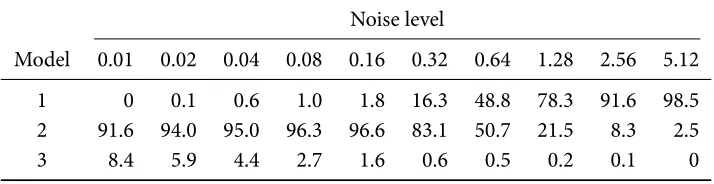
Table 3.1 Frequencies of models selected by aic𝑐(%) for 2,000 pet compartmental model data sets simulated from the three-compartments model.
Noise level
Model 0.01 0.02 0.04 0.08 0.16 0.32 0.64 1.28 2.56 5.12
1 0 0.1 0.6 1.0 1.8 16.3 48.8 78.3 91.6 98.5 2 91.6 94.0 95.0 96.3 96.6 83.1 50.7 21.5 8.3 2.5 3 8.4 5.9 4.4 2.7 1.6 0.6 0.5 0.2 0.1 0
models selected by aic𝑐for 2,000 data sets simulated from the three-compartments model (see Section 2.3) while using the nls estimator. It can be seen that, for data sets with small noise levels (the highest variance of the Normally distributed error added to the simulated time series, with others scaled in proportion), the aic𝑐 method is able to select the two-compartments model with a very high frequency. Though this is not the true model that generated the data, it is very close as the third compartment is difficult to identify (see discussions in [167] and references therein). However, when the noise level increases, the method is unable to identify the second compartment.
3.1.4 Takeuchi’s information criterion
As stated earlier, aic (and some of its refinements such as aic𝑐) depends on the assumption that the candidate models are close to the one that generated the data. However, this might not be the case in reality. In [155], a general derivation from kld to aic was developed. An intermediate result indicated a selection criterion useful when there is considerable model misspecification, formulated as tic,
tic= −2ℓ𝑛(𝜃) + 2 tr(𝐻(𝜃)𝐾(𝜃)−1) (3.10)
where−𝐻(𝜃)is the expectation of the Hessian matrix and𝐾(𝜃)is the variance matrix of the score vector, respectively, that is,
𝐻(𝜃) = − 𝔼𝑔[𝜕
2log 𝑓(𝑋|𝜃)
𝜕𝜃𝜕𝜃𝑇 ] and 𝐾(𝜃) = var𝑔[
𝜕 log 𝑓(𝑋|𝜃)
𝜕𝜃 ], (3.11)
provided that all differentiations and integrations exist. The expectations are taken with respect to the true data generating distribution𝑔. Ideally tic should be eval-uated at the minimizer of the kld,𝜃. In reality, the mle is often used to eval-̃ uate the likelihood function and various estimator of the bias correction term, tr(𝐻( ̃𝜃)𝐾( ̃𝜃)−1), has been developed (see e.g., [32]). If the mle is well behaved [106], then we can substitute the mle into Equation (3.10) and use empirical aver-ages as estimates oftr(𝐻( ̂𝜃)𝐾( ̂𝜃)−1). The explicit form of the bias correction term can also be derived for some models. For example, see [23, sec. 6.6]. This allows more accurate evaluation of tic.
such assumptions and may perform considerably better than aic in the situation of model misspecification.
Unlike the refinements of aic such as aic𝑐, the tic method relies heavily on the assumption of large sample size in order to obtain accurate estimation of the bias term. It is difficult to derive small sample correction for the tic approximation. See also the discussions in [23, sec. 6.7.8]
3.1.5 Cross-validation
Cross-validation has a long history in applied and theoretical statistics. It has been formalized in [51] and [151] (also see the introduction in [151] for an overview of earlier development on this method). The basic idea is to split the data into two parts. One part of the data is used for model fitting and the resulting estimates of parameters are used to predict the other part of the data. By comparing the predictions based on part of the data and the observed other part, the usefulness of the model is determined.
Formally, following [51], let𝑦 = (𝑦1, … , 𝑦𝑛)be the data set and𝑦𝑡 ⊂ 𝑦be a non-empty proper subset. The sub-sample𝑦𝑡is called thetraining setand its complement𝑦𝑣 =𝑦\𝑦𝑡is called thevalidation set. For each model, defined by a parametric distribution with density𝑓(⋅|𝜃), a loss function is defined, say𝛾(⋅|𝜃). The choice of the loss function𝛾is formally arbitrary. It is taken as a measurement of the fitness of the model. A commonly used one is the log-density function, 𝛾(𝑥|𝜃) = − log 𝑓(𝑥|𝜃)[149]. The risk estimator of𝔼𝑔[𝛾(𝑋| ̂𝜃(𝑦))], where𝜃(̂𝑦)is the estimate obtained with all data and the expectation is taken with respect to the unknown distribution𝑔that generates the data, is obtained through averaging over the left-out data,
̂
𝑅𝑣𝑓(𝑦,𝑦𝑡) = 1 |𝑦\𝑦𝑡| ∑
𝑦∈𝑦\𝑦𝑡
𝛾(𝑦| ̂𝜃(𝑦𝑡)) (3.12)
estimator of the risk is defined as,
̂
𝑅cv𝑓 (𝑦, {𝑦𝑡𝑖}𝑚𝑖=1) = 1 𝑚
𝑚 ∑ 𝑖=1
̂
𝑅𝑣𝑓(𝑦,𝑦𝑡𝑖). (3.13)
The model selection proceeds to choose the model with the smallest value of the estimated risk𝑅̂cv𝑓 (𝑦, {𝑦𝑡𝑖}𝑚𝑖=1).
An alternative, as seen in [164], is called cross-validationwith voting. A model with density𝑓1is chosen over a model with density𝑓2if and only if𝑅̂𝑣𝑓
1(𝑦,𝑦 𝑡 𝑖) <
̂
𝑅𝑣𝑓 2(𝑦,𝑦
𝑡
𝑖)for a majority of the partitions of the data𝑦. When there are multiple candidate models, the same paper proposed the following procedure: For each partition of the data𝑦, and the corresponding training set𝑦𝑡𝑖 and validation set 𝑦𝑣𝑖 =𝑦\𝑦𝑡𝑖, a model with the smallest value of𝑅̂𝑣𝑓(𝑦,𝑦𝑡𝑖)is selected. Then the model selected most frequently (the most voted) among all partitions is chosen as the best model.
There are different ways to split the sample. The most commonly used is perhaps theleave-one-outprocedure [151, 51]. In this case, training sets𝑦𝑡𝑖 =𝑦\{𝑦𝑖} for𝑖 = 1, … , 𝑛are used. A more general scheme is that𝑘observations are left out for each training set and all possible combinations are considered [144]. It is clear that𝑘 = 1yields the leave-one-out procedure and for large sample size, a modest 𝑘can lead to higher computational cost as the number of possible partitions is the binomial coefficient. This is also called the𝑘-foldprocedure. Other procedures are also possible. For more information we refer to [150] and [75].
There are also different choices of the loss function𝛾. The one mentioned earlier,𝛾(𝑥|𝜃) = − log 𝑓(𝑥|𝜃), when combined with the leave-one-out procedure, leads to the estimator,
−1 𝑛
𝑛 ∑ 𝑖=1
log 𝑓(𝑦𝑖| ̂𝜃(𝑦𝑡𝑖)) (3.14)
estimator. Given a model𝑦𝑖=𝛽𝑇𝑥𝑖+ 𝜀𝑖, and let𝑦̂𝑖be the predictor of𝑦𝑖obtained with the model fitted with all but the𝑖th observation, i.e., using the leave-one-out procedure, this leads to the press statistic,
press= 𝑛 ∑ 𝑖=1
(𝑦𝑖− ̂𝑦𝑖)2 (3.15)
The model with the smallest press value is selected. This is one of the commonly used model selection methods for regression models.
The performance of cross-validation for model selection depends on both the choice of the loss function and the partition of the sample. There is a large amount of literature on cross-validation for various model selection problems. For some models, specific choice of the function𝛾were proposed, for example, the press statistic shown earlier and its more robust variant such as replacing the squared error by the absolute error [32, sec. 2.9]. Also as argued in the same book, the use of𝛾(𝑥|𝜃) = − log 𝑓(𝑥|𝜃)is a sensible choice for many applications, as the resulting cross-validation estimator can be interpreted as an estimator of the expected relative kld.
3.2 bayesian model comparison
Bayes’ theorem, in its simplest form is stated as below,
Pr(𝐻|𝑦) = Pr(𝑦|𝐻) Pr(𝐻)
Pr(𝑦) (3.16)
where𝑦is the data and𝐻is a hypothesis. Like many other probability theories, technically Bayes’ theorem merely provides a method of accounting for the uncer-tainty. There are different interpretations, rooted in the views of probabilities. See [20, chap. 1] and references therein for discussions on this topic. In this thesis, we are more concerned with the practical applications of the Bayesian model compar-ison technique, its computational difficulties, and its implementation for realistic models. More philosophical issues will not be elaborated in this thesis.
A treatment of Bayesian modeling from a decision-theoretic perspective can be found in [134]. Formal mathematical representations can also be found in [20, sec. 5.1 and sec. 6.1]. Notions of rational decisions in the context of uncertainty were also made precise in the form of axioms in [35, 36]. It is assumed that a rational decision cannot be considered separately from rational beliefs. And rational beliefs should be built upon available information (the data) and any personal preference input (the prior information).
In the remainder of this section, we first introduce the formalization of the model choice problem within the Bayesian framework. It leads to the important Bayes factor, discussed in Section 3.2.2. In Section 3.2.3 we discuss the construction of priors and its particular relevance to the Bayesian model comparison problem.
3.2.1 Model choice problems
parameters conditional upon the model, say𝜋(𝜃𝑘|ℳ𝑘). And each model itself has a prior distribution𝜋(ℳ𝑘). For the purpose of simplicity, all distributions are assumed to be continuous except𝜋(ℳ𝑘), which is assumed to be discrete. According to Bayes’ theorem, the posterior distribution of the parameters and the model, conditional upon the data, is given by the following density, defined on the space⋃𝑘∈u�{ℳ𝑘} × 𝛩𝑘,
𝜋(𝜃𝑘,ℳ𝑘|𝑦) =𝑝(𝑦|𝜃𝑘,ℳ𝑘)𝜋(𝜃𝑘|ℳ𝑘)𝜋(ℳ𝑘)
𝑝(𝑦) , (3.17)
where
𝑝(𝑦) = ∑ 𝑘∈u�
𝑝(𝑦|ℳ𝑘)𝜋(ℳ𝑘), (3.18)
𝑝(𝑦|ℳ𝑘) = ∫ 𝑝(𝑦|𝜃𝑘,ℳ𝑘)𝜋(𝜃𝑘|ℳ𝑘) d 𝜃𝑘. (3.19)
The distribution𝜋(𝜃𝑘,ℳ𝑘|𝑦)is termed thefull posterior. The within model poste-rior distribution of the parameters is given by,
𝜋(𝜃𝑘|𝑦,ℳ𝑘) = 𝑝(𝑦|𝜃𝑘,ℳ𝑘)𝜋(𝜃𝑘|ℳ𝑘)
𝑝(𝑦|ℳ𝑘) . (3.20)
The term𝑝(𝑦|ℳ𝑘)is called themarginal likelihoodor theevidenceof the model. Note that the marginal likelihood is also the normalizing constant of the posterior 𝑝(𝜃𝑘|𝑦,ℳ𝑘).
From Equation (3.17), it is clear that the posterior model probability𝜋(ℳ𝑘|𝑦) is a marginal of the full posterior, and can be calculated given the prior𝜋(ℳ𝑘),
𝜋(ℳ𝑘|𝑦) = 𝜋(ℳ𝑘) ∫ 𝑝(𝑦|𝜃𝑘,ℳ𝑘)𝜋(𝜃𝑘|ℳ𝑘) d 𝜃𝑘
∑𝑙∈u�𝜋(ℳ𝑙) ∫ 𝑝(𝑦|𝜃𝑙,ℳ𝑙)𝜋(𝜃𝑙|ℳ𝑙) d 𝜃𝑙. (3.21)
The Bayesian model choice problem mostly centers around the inference of this posterior model probability. Many methods for computing this probability are re-viewed in Chapter 4. In the remainder of this section, we assume that the calculation of required quantities is possible and accurate.
prediction of future events, etc. The consequences of these actions instead of the chosen model itself are of interest. Therefore, from a decision-theoretic perspective, the “best” model should maximize the utility for some quantity of interest. However, in practice it is common to ignore the actions following the model selection and the sole interest is the true model, sayℳ𝑡. This is because the Bayesian framework is often used to simultaneously provide parameter estimation, model selection, model averaging and other inferences. It is difficult to define a criterion that chooses models best for all these purposes. In the simplified setting, where only the true model is of interest, it is natural to define a zero-one utility function, say𝑢(ℳ𝑘,ℳ𝑡),
𝑢(ℳ𝑘,ℳ𝑡) = { { { { {
0, ifℳ𝑘=ℳ𝑡,
1 otherwise.
(3.22)
It is easy to see that the modelℳ𝑘that maximizes the expected utility given data 𝑦is the model with the highest posterior probability𝜋(ℳ𝑘|𝑦)[20, chap. 6]. Also see [134, sec. 7.2.1] for an in-depth discussion of the difficulties of the Bayesian formulation in the model choice problem and the reason why such a simplified maximum posterior probability approach.
It should be noted that the use of the zero-one utility is only valid if the true modelℳ𝑡belongs toℳ. Otherwise, the utility is always zero for all models. In what follows, we presume that our aim is to find the model with the highest posterior probability.
Bayesian model selection can be attractive for a few reasons. First, it pro-vides a natural probabilistic interpretation of the results. It is very easy to account model uncertainty within this framework. When there are more than one models well supported by the data and it is uncertain which one should be chosen as the best model, the posterior model probabilities can be used as weights to construct weighted estimator. This leads to Bayesian model averaging. See, e.g., [130, 33, 41], for more discussions and examples.
for the pet compartmental model showing that Bayesian model selection indeed provides better results compared to methods such as aic.
Third, and perhaps a more important factor, the Bayesian framework can be applied to a wider range of applications compared to methods based on asymptotic behaviors of the data. There are very minimal assumptions about the models under consideration. Model selection methods reviewed earlier often require the good behavior of an estimator, or a sufficient large sample size etc. In contrast, within Bayesian framework, the regularity of the likelihood function is not an issue as long as the integrations in Equation (3.21) are finite. In addition, though a large sample size can be beneficial in the sense that it can reduce the uncertainty of the model selection results, it is not necessary. The uncertainty of model selection is well accounted within the Bayesian framework and improvements can be obtained through model averaging as mentioned earlier. These advantages allow Bayesian model selection to be successfully applied to a wide range of applications.
3.2.2 Bayes factor
When the model setℳis finite, we can find the model with the highest posterior probability by comparing models pairwise. To compare the posterior probabilities of two models, sayℳ𝑘
1andℳ𝑘2, one only needs to compute their ratio. Recall Equation (3.21), the ratio can be written as,
𝜋(ℳ𝑘1|𝑦) 𝜋(ℳ𝑘2|𝑦) =
𝜋(ℳ𝑘1) 𝜋(ℳ𝑘2)
∫ 𝑝(𝑦|𝜃𝑘1,ℳ𝑘1)𝜋(𝜃𝑘1|ℳ𝑘1) d 𝜃𝑘
∫ 𝑝(𝑦|𝜃𝑘
2,ℳ𝑘2)𝜋(𝜃𝑘2|ℳ𝑘2) d 𝜃𝑘
=𝜋(ℳ𝑘1)
𝜋(ℳ𝑘2)𝐵𝑘1𝑘2, (3.23)
where
𝐵𝑘1𝑘2 = ∫ 𝑝(𝑦|𝜃𝑘1,ℳ𝑘1)𝜋(𝜃𝑘1|ℳ𝑘1) d 𝜃𝑘1 ∫ 𝑝(𝑦|𝜃𝑘2,ℳ𝑘2)𝜋(𝜃𝑘2|ℳ𝑘2) d 𝜃𝑘2 =
𝑝(𝑦|ℳ𝑘1)
𝑝(𝑦|ℳ𝑘2) (3.24)
Table 3.2 Jeffreys’ intepretation of the Bayes factor.
log10𝐵𝑘1𝑘2 𝐵𝑘1𝑘2 Evidence in favor of model𝑀𝑘1
0to1/2 1to3.2 Not worth more than a bare mention 1/2to1 3.2to10 Substantial
1to2 10to100 Strong
> 2 > 100 Decisive
the computation of the marginal likelihood for each modelℳ𝑘∈ℳ,
𝑝(𝑦|ℳ𝑘) = ∫ 𝑝(𝑦|𝜃𝑘,ℳ𝑘)𝜋(𝜃𝑘|𝑘) d 𝜃𝑘.
It is obvious that𝐵𝑖𝑗= 𝐵𝑖𝑘𝐵𝑘𝑗, and thus the Bayes factor approach is equivalent to choosing the model with the highest marginal likelihood provided that the model prior distribution𝜋(ℳ𝑘)is uniform, as long as the model setℳis finite.
The Bayes factor,𝐵𝑘
1𝑘2, can be interpreted as the evidence provided by the data in favor of modelℳ𝑘1against modelℳ𝑘2. As noted earlier, the marginal like-lihood𝑝(𝑦|ℳ𝑘)is also called the evidence supporting modelℳ𝑘. Jeffrey suggested that the Bayes factor can be interpreted on alog10scale [88]. The interpretations are reproduced in Table 3.2. The interpretation of the Bayes factor can be application de-pendent. The Jeffreys’ interpretation, and a similar scale based on2 log 𝐵𝑘1𝑘2, which is on the same scale as the likelihood ratio test [96], are only general guidelines. Other interpretations can be more suitable for specific applications. For example, [96] mentioned that for forensic evidence to be conclusive in a criminal trial, the posterior odds of guilt against innocence needs to be at least 1,000.
The calculation of the Bayes factor can be made exact using analytical results only occasionally. In most applications of interest, approximations have to be used. Two approaches are widely used. One is to use Monte Carlo approximations. An-other is based on the asymptotic behavior of the Bayes factor. Two of the later are reviewed here.
Bayesian information criterion
The Bayesian information criterion (bic) was developed as a large sample approxi-mation to the marginal likelihood𝑝(𝑦|𝜃𝑘,ℳ𝑘)[141]. The bic is defined as,
bic= −2ℓ𝑛( ̂𝜃𝑘) + 𝑘 log(𝑛), (3.25)
whereℓ𝑛( ̂𝜃𝑘)is the log-likelihood function evaluated at the mle,𝑘is the number of parameters to be estimated and𝑛is the number of observations. The bic strategy chooses the model with the smallest value of bic. A derivation of bic can be found in [32, sec. 3.2].
Similar to aic, bic assumes that the sample size is large enough in order to approximate the marginal likelihood properly. In addition, bic also assumes “good behavior” of the likelihood function in the sense that the mle is in the high posterior probability region. These assumptions restrict the use of bic in some situations. See [18] for examples where the irregularity of the likelihood function caused the bic method unable to give reasonable results. There are other criticism of the bic strategy. For example [134, sec. 7.2.3] argued that the bic strategy eliminated the subjective input into the Bayes modeling since the value of bic does not depend on the prior distribution. However this is equally argued as an advantage of this strategy in the case that priors, to which the Bayes factors can be very sensitive, are hard to specify.
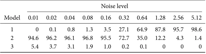
Table 3.3 Frequencies of models selected by bic (%) for 2,000 pet compartmental model data sets simulated from the three-compartments model.
Noise level
Model 0.01 0.02 0.04 0.08 0.16 0.32 0.64 1.28 2.56 5.12
1 0 0.1 0.8 1.3 3.5 27.1 64.9 87.8 95.7 98.6 2 94.6 96.2 96.1 96.8 95.5 72.7 35.0 12.2 4.3 1.4 3 5.4 3.7 3.1 1.9 1.0 0.2 0.1 0 0 0
contrast to aic (see discussions in Section 3.1.2), bic is less subject to overfitting. On the other hand, it may not be as efficient as aic for some applications. For example, in [105] it was shown that for autoregressive process and some other time series applications, bic is not efficient in the sense that bic may not choose the model that minimizes the prediction error. In [32, sec. 4.7], it was also shown that bic is not efficient for regression variable selection.
Table 3.3 shows the frequencies of models selected by the bic for 2,000 pet data sets simulated from the three-compartments model (see Section 2.3) while using the nls estimator. Compared to the use of aic𝑐(Table 3.1), the results are quite similar though bic does tend to select lower order models more frequently. Intuitively, bic penalizes model complexity more than aic for𝑛 ≥ e2 ≈ 7.4(and thus the penalty term𝑘 log(𝑛) > 2𝑘).
Laplace approximation
An alternative large sample approximation of the marginal likelihood is given by [159],
(2𝜋)𝑑𝑘/2√|(−𝐻( ̃𝜃))−1|𝑝(𝑦| ̃𝜃
𝑘,ℳ𝑘)𝜋( ̃𝜃𝑘|ℳ𝑘) (3.26)
the likelihood function is close to Normal [96].
Often the maximizer of the posterior density is not easily obtained. A variant of the Laplace approximation is to use the mle instead. For a sufficient large sample size, the posterior is likely to peak at the same region as the likelihood function.
Though less commonly used than the bic approximation, the Laplace approx-imation does not eliminate the effects of priors. For some applications, it provides a low cost (compared to simulation techniques) alternative for evaluating the Bayes factor over a range of priors.
3.2.3 Choice of priors
Conjugate priors
A conjugate prior, say𝜋(𝜃𝑘|ℳ𝑘), for a parametric model with a likelihood function 𝑝(𝑦|𝜃𝑘,ℳ𝑘), is one such that the posterior𝜋(𝜃𝑘|𝑦,ℳ𝐾)belongs to the same family of distributions as the prior. In [20, sec. 5.2] it was argued that a conjugate prior re-duces the input of prior information to only the choice of parameter values and thus cannot be fully justified from a subjective perspective. Though their mathematical simplicity makes them attractive, for many applications of interest it is difficult to find such priors.
Non-informative priors
In situations where no or little prior information is available, the so-called “non-informative” priors are often used. Many of them are derived from the data or the likelihood function of the models.
Flat tails The simplest form is a uniform distribution or some distribution with
flat tails such as a Cauchy distribution. This choice can provide a robust prior in the sense that outliers and misspecification of priors will not affect the results significantly. For example, see [124] and [42] for analysis of the use of the Student𝑡 distribution as the prior of location parameters such as the mean of a Normal distribution.
Jeffreys priors Jeffreys priors [87] have the form,
𝜋(𝜃𝑘|ℳ𝑘) ∝ √|𝐼(𝜃𝑘)| (3.27)
where
𝐼(𝜃𝑘) = − 𝔼𝑦[𝜕
2log 𝑝(𝑦|𝜃 𝑘,ℳ𝑘)
𝜕𝜃𝑘𝜕𝜃𝑇𝑘 ] (3.28)
in the sense that, for a one-to-one transformation𝜙𝑘= ℎ(𝜃𝑘), we have the Jacobian transformation,
𝐼(𝜙𝑘) = (𝐽(ℎ−1(𝜙𝑘)))𝑇𝐼(ℎ−1(𝜙𝑘))(𝐽(ℎ−1(𝜙𝑘)))
where𝐽(ℎ−1(𝜙𝑘))is the Jacobian matrix . For𝜃𝑘 = ℎ−1(𝜙𝑘), it follows,
𝜋(𝜙𝑘) ∝ √|𝐼(𝜃𝑘)||𝐽(ℎ−1(𝜙
𝑘))| ∝ 𝜋(𝜃𝑘)| 𝜕𝜃𝑘 𝜕𝜙𝑘|
where the last term is the determinant of the Jacobian transformation. The above expression states that the Jeffreys prior of the transformed parameter𝜙𝑘is the same as the one obtained by changing variable of the Jeffreys prior of𝜃𝑘. In other words, a change of variable does not change the prior under the Jeffreys rule. Another informal interpretation is that, the prior should contain no more information than the observed data do. The Fisher information is widely accepted as an indicator of the amount of information brought by the model about the parameter𝜃𝑘given the data [45]. Therefore, intuitively values of𝜃𝑘for which𝐼(𝜃𝑘)are large are more likely than those for which𝐼(𝜃𝑘)are small.
arbitrarily closely approximate𝜋(𝑥) ∝ 1/𝑥, which is often seen as the Jeffreys prior for scale parameters, such as the precision parameter of a Normal distribution.
Reference priors Another class of non-informative priors is calledreference priors,
introduced in [19]. Reference priors aim to derive priors such that the distance between the posterior and prior is maximized, usually measured in terms of the Kullback-Leibler divergence [102] (also see Section 3.1.1). In some sense, a reference prior is the least informative prior. See [14, 16, 15] and [20, sec. 5.4] for more information on this class of priors.
Another form of the reference priors is to partition the parameter vector 𝜃𝑘 = (𝜃(1)𝑘 , 𝜃(2)𝑘 )where 𝜃(1)𝑘 is the parameter of interest and𝜃(2)𝑘 is the nuisance parameter. First𝜋(𝜃(2)𝑘 |𝜃(1)𝑘 ,ℳ𝑘)is defined as the Jeffreys prior associated with 𝑝(𝑦|𝜃𝑘,ℳ𝑘)when𝜃(1)𝑘 is fixed. Then define the marginal,
̃
𝑝(𝑦|𝜃(1)𝑘 ,ℳ𝑘) = ∫ 𝑝(𝑦|𝜃𝑘,ℳ𝑘)𝜋(𝜃(2)𝑘 |𝜃(1)𝑘 ,ℳ𝑘) d 𝜃(2)𝑘 , (3.29)
and compute the Jeffreys prior𝜋(𝜃(1)𝑘 |ℳ𝑘)associated with𝑝(̃𝑦|𝜃(1)𝑘 ,ℳ𝑘). By us-ing the Jeffreys prior, given fixed parameter of interest, the effects of the nuisance parameter is eliminated.
Using non-informative priors for the pet compartmental model In [167] results of
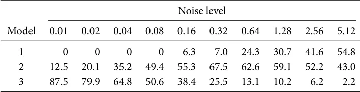
Table 3.4 Frequencies of models selected by the Bayes factor (vague priors) (%) for 2,000 pet compartmental model data sets simulated from the three-compartments model
Noise level
Model 0.01 0.02 0.04 0.08 0.16 0.32 0.64 1.28 2.56 5.12
1 0 0 0 0 6.3 7.0 24.3 30.7 41.6 54.8 2 12.5 20.1 35.2 49.4 55.3 67.5 62.6 59.1 52.2 43.0 3 87.5 79.9 64.8 50.6 38.4 25.5 13.1 10.2 6.2 2.2
For more noisy data, it is expected the second and third compartments are difficult to identify. Overall, the results are much more satisfactory than those of aic𝑐and bic.
Informative priors
When the parameters bear real world meaning, it may be possible to construct informative priors. For some applications, calibrating an informative prior requires substantial expertise and some model specific information. Nonetheless, there are also some general methods.
When the parameter space is finite, it might be possible to obtain subjective evaluation of the probabilities of the different values of the parameter. When the space is uncountable, the problem is obviously more complicated. One simple approach is to partition the parameter space and determine the probabilities of the parameter falling into each of the partition [134, sec. 3.2.2].
A more systematic approach is themaximum entropy priors[86]. Assume that some characteristics of the parameter vector𝜃𝑘in the modelℳ𝑘are known in the form of prior expectations,
𝔼𝜋[ℎ𝑖(𝜃𝑘)|ℳ𝑘] = 𝛾𝑖, for𝑖 = 1, … , 𝐾 (3.30)
![Figure 4.5Convergence dren [0.9, 1.1]avalue within the range ofre no appatcspos burn thr-in sampcompavariance o pet usingf](https://thumb-us.123doks.com/thumbv2/123dok_us/9571212.461210/86.612.120.462.83.189/figure-convergence-appatcspos-sampcompavariance-iagnosti-rtments-estimates-samples.webp)