Linear scaling time dependent density functional theory beyond the Tamm Dancoff approximation : obtaining efficiency and accuracy with in situ optimised local orbitals

Original citation:

Zuehlsdorff, T. J., Hine, Nicholas, Payne, M. C. and Haynes, P. D.. (2015) Linear-scaling time-dependent density-functional theory beyond the Tamm-Dancoff approximation : obtaining efficiency and accuracy with in situ optimised local orbitals. The Journal of Chemical Physics, 143 (20). 204107.

Permanent WRAP url:

http://wrap.warwick.ac.uk/75015

Copyright and reuse:

The Warwick Research Archive Portal (WRAP) makes this work by researchers of the University of Warwick available open access under the following conditions. Copyright © and all moral rights to the version of the paper presented here belong to the individual author(s) and/or other copyright owners. To the extent reasonable and practicable the material made available in WRAP has been checked for eligibility before being made available.

Copies of full items can be used for personal research or study, educational, or not-for-profit purposes without prior permission or charge. Provided that the authors, title and full bibliographic details are credited, a hyperlink and/or URL is given for the original metadata page and the content is not changed in any way.

Publisher statement:

© (2015) AIP Publishing. This article may be downloaded for personal use only. Any other use requires prior permission of the author and AIP Publishing.

The following article appeared in (citation above) and may be found at http://dx.doi.org/10.1063/1.4936280

A note on versions:

The version presented here may differ from the published version or, version of record, if you wish to cite this item you are advised to consult the publisher’s version. Please see the ‘permanent WRAP url’ above for details on accessing the published version and note that access may require a subscription.

Linear-scaling time-dependent density-functional theory beyond

the Tamm-Dancoff approximation: obtaining efficiency and

accuracy with

in situ

optimised local orbitals

T. J. Zuehlsdorff,1,∗ _{N. D. M. Hine,}2 _{M. C. Payne,}1 _{and P. D. Haynes}3, 4, 5 1_{Cavendish Laboratory, J. J. Thomson Avenue, Cambridge CB3 0HE, UK}

2_{Department of Physics, University of Warwick, Coventry, CV4 7AL}

3_{Department of Materials, Imperial College London,}

Exhibition Road, London SW7 2AZ, UK

4_{Department of Physics, Imperial College London,}

Exhibition Road, London SW7 2AZ, UK

5_{Thomas Young Centre for Theory and Simulation of Materials,}

Imperial College London, Exhibition Road, London SW7 2AZ, UK

Abstract

We present a solution of the full time-dependent density-functional theory (TDDFT) eigenvalue equation in the linear response formalism exhibiting a linear-scaling computational complexity with system size, without relying on the simplifying Tamm-Dancoff approximation (TDA). The implementation relies on representing the occupied and unoccupied subspace with two different sets ofin situ optimised localised functions, yielding a very compact and efficient representation of the transition density matrix of the excitation with the accuracy associated with a systematic basis set. The TDDFT eigenvalue equation is solved using a preconditioned conjugate gradient algorithm that is very memory-efficient. The algorithm is validated on a small test molecule and a good agreement with results obtained from standard quantum chemistry packages is found, with the preconditioner yielding a significant improvement in convergence rates. The method developed in this work is then used to reproduce experimental results of the absorption spectrum of bacteriochlorophyll in an organic solvent, where it is demonstrated that the TDA fails to reproduce the main features of the low energy spectrum, while the full TDDFT equation yields results in good qualitative agreement with experimental data. Furthermore, the need for explicitly including parts of the solvent into the TDDFT calculations is highlighted, making the treatment of large system sizes necessary that are well within reach of the capabilities of the algorithm introduced here. Finally, the linear-scaling properties of the algorithm are demonstrated by computing the lowest excitation energy of bacteriochlorophyll in solution. The largest systems considered in this work are of the same order of magnitude as a variety of widely studied pigment-protein complexes, opening up the possibility of studying their properties without having to resort to any semiclassical approximations to parts of the protein environment.

I. INTRODUCTION

The study of optical properties of large complex systems is of increasing interest in

com-putational biology, with most efforts being focused on understanding large pigment-protein

complexes (PPCs)[1–5]. These systems turn up in a variety of different roles in nature, from

biosensors to light-harvesting and linker complexes in photosynthetic bacteria andab-initio

computational studies can play a key role in gaining a deeper insight into the mechanisms

governing them. However, PPCs are generally characterised by the fact that the protein

en-vironment plays an important role in influencing the absorption properties of the pigment,

creating the need for large-scale quantum mechanical calculations that are

computation-ally challenging[2–4]. In general, time-dependent density-functional theory (TDDFT)[6],

the time-dependent extension to ground-state density-functional theory (DFT)[7, 8], is

con-sidered the method of choice when treating this class of systems, mainly due to the good

balance between computational cost and achievable accuracy for most common choices of

exchange-correlation functionals.

In recent years there have been a number of developments in computational algorithms[9–

11] that have helped to make medium-sized systems routinely accessible to TDDFT.

How-ever, most common approaches to solving the low energy spectrum of a system using TDDFT

show a computational complexity of at least O(N3_{) with system size, imposing an upper}

limit on the system sizes that can be realistically studied and effectively ruling out a full

treatment of the PPCs mentioned above. To treat these large biological systems explicitly

in TDDFT, it is necessary to make use of computational approaches that scale linearly with

system size.

TDDFT is generally considered in two different flavours. The time domain approach,

where the Kohn-Sham equations are propagated explicitly in time[12], and the linear

re-sponse approach[13], where the excitation energies of the system can be recast as the

so-lutions to an effective eigenvalue equation[14, 15]. The time-domain approach can yield

the entire spectrum of the system via a Fourier transform to the frequency domain, is

non-perturbative and can thus be applied to problems beyond the linear response regime.

However, it comes with the disadvantage that the Kohn-Sham equations have to be

propa-gated sufficiently long to obtain narrow line-widths and dark states cannot be resolved. The

dark states and triplet transitions that are of interest in some photochemical processes. For

this reason, we focus on the linear response flavour of TDDFT for the purpose of this work.

In the time-domain TDDFT approach, an O(N) computational effort with system size can

be achieved by extending linear-scaling techniques known from ground-state DFT to the

time-dependent Kohn-Sham equations[16–18]. In the linear response approach, algorithms

capable of solving for the lowest eigenvalues of the TDDFT eigenvalue equation are also

known[19–21], opening up the possibility of a direct computation of excited states in large

pigment-protein complexes without relying on additional semi-classical approximations.

The linear response TDDFT equation is a non-Hermitian eigenvalue problem, causing it

to be difficult to solve using standard off-the-shelf eigenvalue solvers. A simplifying

approx-imation, known as the Tamm-Dancoff approximation (TDA)[22, 23], recasts the problem

into an Hermitian one but its effect on excitation energies and oscillator strengths is not

straightforwardly understood. In this work, we introduce a linear-scaling implementation of

full TDDFT in the framework of the ONETEP code[24], without relying on the TDA, as was

required in a previous approach[20]. We test the performance of the algorithm on a number

of large scale systems and specifically investigate the quality of the full TDDFT eigenstates

to those obtained within the TDA. The largest systems considered explicitly in this work are

of similar size as a number of widely studied PPCs (see for example [2, 3]), thus highlighting

the capabilities of the algorithm developed here to enable a fullyab-initio treatment of this

class of systems.

This work is organised as follows: Section II focuses on providing a short overview of the

theoretical background necessary for the main results presented in this work, with sections

II A and II B introducing the linear response formalism to TDDFT, both in the form of a

matrix eigenvalue equation and an effective variational principle. Section II C then provides

a short summary of theONETEPcode in which the algorithm presented is implemented, as well

as an overview over a solution to the Tamm-Dancoff eigenvalue problem[20]. In section III,

the linear-scaling solution to the full TDDFT eigenvalue equation is outlined, with a special

focus being placed on the appropriate choice of preconditioner (III B) for the conjugate

gradient algorithm. The power of the methodology developed here is demonstrated on a

small test system by comparison to accurate benchmark results (IV A), before moving on

to a realistic system of bacteriochlorophyll a in an organic solvent. It is shown that the

systems inaccessible by conventional approaches.

II. THEORETICAL BACKGROUND

In this section we briefly introduce the theoretical background of linear response TDDFT.

We consider a Kohn-Sham system with ground-state density ρ{0} and occupied and unoc-cupied Kohn-Sham states{ψKS

vσ}and {ψcσKS}respectively, where σ denotes a spin index. We

limit the discussion to isolated systems, such that the Kohn-Sham eigenstates can be chosen

to be real. Furthermore, only semi-local exchange-correlation functionals in the adiabatic

approximation will be considered, thus ignoring any long-range and memory effects. While

memory effects are routinely ignored in standard TDDFT implementations, long-range

in-teractions can be included in form of hybrid functionals and are known to yield a better

description for excitations in infinite systems and charge-transfer states, where semi-local

exchange correlation functionals are known to fail[15, 25]. However, for the purpose of this

work the main focus is on excitations that retain a localised character and that are thus well

described by semi-local functionals.

A. Linear response TDDFT

In linear response TDDFT, the individual excitation energies of the system can be

ob-tained by solving a non-Hermitian eigenvalue equation of the form[14, 15]



 A B

−B −A

 

 X

Y  =ω

 X

Y 

 (1)

Here, A and B denote block matrices that can be conveniently expanded in a basis of

unoccupied and occupied eigenstates of the ground state Kohn-Sham system:

Acvσ,c′v′σ′ = δσσ′δcc′δvv′(ϵKSc′σ′ −ϵ KS

v′σ′) +Kcvσ,c′v′σ′ (2)

Bcvσ,c′v′σ′ = Kcvσ,c′v′σ′. (3)

where{ϵKS

cσ}and {ϵKSvσ} denote the eigenvalues associated with the unoccupied and occupied

Kohn-Sham states respectively. The eigenvectors are made up of two different components

X and Y that can be thought of as excitation and de-exitation contributions to the

eigenvalue matrix can be characterised by a diagonal part consisting of Kohn-Sham

tran-sitions between occupied and unoccupied states and off-diagonal coupling terms described

through the coupling matrixK. The exact form ofKdepends upon the exchange-correlation

functional used. Here, we will limit our attention to (semi)-local functionals in the adiabatic

approximation, in which case the matrix elements of K can be expressed as

Kcvσ,c′v′σ′ = ∫

d3rd3r′ψ_cσKS(r)ψ_vσKS(r)

×

[

1 |r−r′| +

δ2_E xc δρσ(r)δρσ′(r′)

ρ{0}

]

ψ_cKS′_σ′(r′)ψ_vKS′_σ′(r′) (4)

where Exc is the exchange-correlation energy. In the remaining part of this work, all spin

indices will be dropped for convenience.

From the structure of Eq. 1 it can be seen that the TDDFT eigenvalue equation has

solutions in the positive and negative frequency domain. These positive and negative

fre-quencies can be interpreted as excitation and de-excitation energies [15]. Note that due to

the structure of the equation, the positive and negative eigenvalue solutions are coupled via

the block matrix B. Assuming that the coupling of excitations to the de-excitation part

of the full TDDFT spectrum is small, one can set the coupling matrices B to zero, which

causes a complete decoupling of the excitation and de-excitation part of the spectrum. The

positive excitation energies can then be solved for via the Hermitian eigenvalue equation

AX=ωX. (5)

Solving Eq. 5 instead of Eq. 1 is referred to as the Tamm-Dancoff approximation

(TDA)[22, 23]. While the TDA is often reported to yield reliable excitation energies in

many situations[23], the structure of the equation violates both time-reversal symmetry and

important sum rules related to the oscillator strengths[26] of the excitations. Furthermore,

there are known cases where the TDA yields to significant errors in excitation energies[27],

making a treatment of the full eigenvalue problem desirable. However, as will be discussed

in more detail in the next section, the main disadvantage of a full treatment of the TDDFT

eigenvalue equation originates from the fact that Eq. 1 constitutes a non-Hermitian

eigen-value problem, meaning that a variety of standard numerical methods for computing the

B. Iterative solutions to the TDDFT equation

The dimensions of the TDDFT eigenvalue equation grow as O(N2_{) with system size,}

making a direct diagonalisation of the matrices in Eq. 1 or Eq. 5 undesirable for larger

systems. Furthermore, one is often interested in a relatively small number of low energy

excited states in the visible or ultraviolet energy range of a system, such that the computation

of high energy excited states is unnecessary. The best approach to tackle the TDDFT

eigenvalue problem for real systems of interest is thus to use iterative methods in order to

calculate the lowest few excited states.

Within the TDA, such an iterative scheme is straightforwardly defined, since the

Hermi-tian properties of the block matrix A allow for the definition of the lowest excitation of the

system via a variational principle:

ω_minTDA = min

X ΩTDA(X) = minX

X†AX

X†X . (6)

From this definition, the gradient of the Rayleigh-Ritz functional ΩTDA(X) with respect to X can then be straightforwardly computed

∂ΩTDA(X)

∂X =gTDA=

2

X†X [

AX− X †_AX

X†X X ]

. (7)

This gradient can be used as a steepest-descent search direction in a conjugate gradient

algorithm to optimise a random starting vector Xguess until the lowest eigenstate ωTDAmin has

been obtained. Note that in order to compute the gradient in Eq. 7, it is only required to

evaluate the matrix-vector product AX. This means that A does not have to be explicitly

calculated or stored during the calculation, which is prohibitive for large systems.

The definition of the lowest eigenvalue of the Tamm-Dancoff TDDFT equation via the

variational principle relies on the fact that it constitutes an Hermitian eigenvalue problem

and is thus not generally possible for the full TDDFT equation. It was however pointed out

by Thouless[28] that since the blocks A and B of the full TDDFT equation are Hermitian,

a variational principle can be formulated for its lowest positive eigenstate via:

ωmin = min (X Y)

ΩThou(X,Y)

= min

(X Y) (

X† Y† )

A B B A

 

 X

Y  

The numerator of the above expression is guaranteed to be positive semi-definite for

(semi)-local exchange-functionals, while the denominator is forced to be positive by taking the

absolute value.

While it is possible to use the above variational principle to directly obtain the lowest

excited state of the full TDDFT equation, the Thouless functional is not the most ideal

formulation of the problem in the context of semi-local exchange-correlation functionals (see

Sec. III A). A more computationally efficient reformulation was introduced by Tsiper [29] by

noticing the equivalence of the full TDDFT eigenvalue problem to that of a set of classical

harmonic oscillators. As a first step, one introduces the effective vectors p = X−Y and

q=X+Y. It can then be easily shown that the Thouless functional can be rewritten as:

ωmin = min

(p q)ΩTsip(p,q)

= min

(p q) (

p† q† )

A−B 0

0 A+B

 

 p

q  

|p†q+q†p| . (9)

Here, the variational principle is again only defined for the lowestpositive excitation of the

system. Just like in the Thouless functional, the numerator of the functional is guaranteed

to be positive-semidefinite. The denominator has to be forced to stay positive by taking the

absolute value, since p†q+q†p is not guaranteed to be positive-semidefinite.

While the variational principles in Eqns. 6 and 9 are written in terms of the lowest

excitation of the system only, the concept can be straightforwardly extended to higher

excitations. In order to converge the second-lowest excitation ω2 of the system, the same

effective functional of Eqn. 9 can be used in full TDDFT, with the additional constraint that

p₂ and q₂, the trial vectors associated withω2 obey an effective orthogonality constraint of

the form

p†₁q₂+q†₁p₂= 0 (10)

wherep₁ and q₁ are taken to denote the vectors associated withωmin, the lowest excitation

of the system. The principle can be extended to an arbitrary number of excited states to be

C. Tamm-Dancoff TDDFT in the ONETEP code

The linear-scaling solution to the full TDDFT equation developed in this work (see

Sec. III) is implemented in the ONETEP code[24]. As with other linear-scaling DFT

ap-proaches, any reference to individual Kohn-Sham states {ψKS

i } is given up in favour of a

collective representation in the form of the single particle density matrixρ{v}_(r,r′_{) such that}

ρ{v}(r,r′) =

N∑occ

v

ψ_vKS(r)ψKS_v (r′)

= ∑

αβ

ϕα(r)P{v}αβϕβ(r′) (11)

where {ϕα(r)} denotes a set of in situ optimised[24] localised atom-centered support

func-tions referred to as non-orthogonal generalised Wannier funcfunc-tions (NGWFS)[33] and P{v} is

the single particle density matrix in the representation of those NGWFs. Linear scaling of

computational cost with system size is then obtained by exploiting the fact that the

ground-state density matrix decays exponentially for any system with a band gap, causing P{v} to

be sparse for sufficiently large system size[34, 35].

Thein situoptimisation of the support functions{ϕα}means that only a minimal number

of functions is required to accurately span the occupied subspace, but the unoccupied

sub-space is generally badly represented[30]. This issue is overcome by optimising a second set

of NGWFs {χα} for a low energy subset of the unoccupied subspace that is represented by

the effective density matrix P{c}[30]. It has been demonstrated[20] that the compact sets of

support functions{ϕα} and {χβ} provide a very good representation for low energy excited

states as calculated in the TDA. Defining an effective response density ρ{1}_{(r) associated}

with a TDA eigenvectorX such that

ρ{1}(r) = ∑

c,v

ψKS_c (r)XcvψvKS(r)

= ∑

αβ

χα(r)P{1}αβϕβ(r) (12)

it becomes clear that the effective response density matrix P{1} is the representation of X

in mixed unoccupied-occupied NGWF space[20]. The matrix-vector product f = AX can

then be directly constructed in NGWF space as

fχϕ_TDA = P{c}HχP{1}−P{1}HϕP{v}

+P{c} (

V{_SCF1}χϕ [

P{1} ])

Here, Hχ and Hϕ denote the ground state Kohn-Sham Hamiltonian in the {χα} and {ϕβ}

representation respectively. V{_SCF1}χϕ [

P{1} ]

is the self-consistent field response of the system

due to a perturbation ρ{1}_{(r) in the ground state density[20] and is the result of X acting}

on the coupling matrix K in mixed unoccupied-occupied NGWF space. Note that fχϕ_TDA

represents a contravariant tensor quantity and has to be multiplied by Sχ and Sϕ from the

left and right respectively to obtain a covariant quantity (see [20] for further details). The

lowest excitation energy of the system can then be written as

ω_minTDA = min

P{1}ΩTDA

[ P{1}

]

= Tr

[

P{1}†SχfχϕSϕ ]

Tr

[

P{1}†SχP{1}Sϕ

] (14)

where Sχ and Sϕ denote the overlap matrices of the {χα} and {ϕβ} NGWF representation

respectively. Higher excited states can be obtained from the same variational principle

by enforcing an orthogonality constraint between all excited states. If all involved density

matrices P{1}, P{v} and P{c} can be treated as sparse for sufficiently large system size[52], evaluating Eqs. 13 and 14 scales as O(N) with system size and ωTDA

min can be computed in

linear-scaling effort using standard iterative approaches.

The above formulation yields accurate excitation energies if X is well-represented by

the low energy subset of unoccupied states for which P{c} is optimised. However, in many

scenarios it is desirable to include higher energy unoccupied states in an approximate manner

to achieve convergence[20, 31]. One straightforward way of doing so is to introduce the joint

unoccupied-occupied representation{φα}={ϕβ}⊕{χγ}and to redefineP{c} via a projector

onto the entire unoccupied subspace representable by {φα}[31]:

P{c} = (Sφ)−1−(Sφ)−1SφϕP{v}Sϕφ(Sφ)−1. (15)

Here, the elements of Sφϕ are given by S_αβφϕ=⟨φα|ϕβ⟩. While using the joint representation

for the unoccupied subspace instead of {χα} roughly doubles the computational cost

com-pared to using {χα}, it yields consistently good TDDFT excitation energies[31, 32] and will

be used throughout in Sec. IV. However, for the purpose of clarity in outlining the

linear-scaling TDDFT algorithm in Sec. III, we shall use{χα}to label the unoccupied space, noting

III. FULL TDDFT IN ONETEP

In this section, we will outline a conjugate gradient algorithm to compute the lowest

Nω excited states of the full TDDFT equation. While other iterative eigensolvers like the

Lanczos and Davidson algorithms and multishift methods have been applied to this

prob-lem, both in the framework of standard cubic scaling[9, 11] and O(N)[19] approaches, the

conjugate gradient method is chosen here for both its good performance in the TDA[20] and

its low memory requirements suitable for large scale applications. A special focus will be put

on an effective preconditioning scheme, as well as the linear-scaling properties of the

algo-rithm. As in the previous section, the discussion is limited to semi-local exchange-correlation

functionals only.

A. The Tsiper functional in mixed {χα}-{ϕβ} NGWF space

The key to obtaining a linear-scaling implementation of the full TDDFT equation is to

rewrite the Tsiper functional in the same compact, localised NGWF representation that has

been used to rewrite the Tamm-Dancoff functional in Eq. 14. For this purpose, we define

f_Tsip as

f_Tsip=

 fp

fq  =



A−B 0

0 A+B

 

 p

q  =



Ap−Bp Aq+Bq



 (16)

Following analogous steps to the derivation of the linear-scaling solution to the TDA

eigen-value equation[20], we define the effective response density matrices P{p} and P{q} and

response densities ρ{p}(r) and ρ{q}(r) such that

ρ{p}(r) = ∑

c,v

ψKS_c (r)p_cvψ_vKS(r)

= ∑

αβ

χα(r)P{p}αβϕβ(r) (17)

with ρ{q}_{(r) following an analogous definition. Thus P}{p} _{and P}{q} _{are the matrices p and}

q in {χα}-{ϕβ} NGWF representation. Just like P{1}[20], P{p} and P{q} have to follow an

effective invariance constraint in order to be valid response density matrices, which originates

from the orthogonality between the unoccupied and occupied Kohn-Sham spaces in which

p and q are represented. For P{p}, the invariance constraint can be written as

with an identical statement forP{q}.

From Sec. II C, the action of A acting on some vector X written in {χα}-{ϕβ} NGWF

space is already known. Using Eq. 13, it is straightforward to rewritef_Tsip in{χα}and {ϕβ}

representation such that

fχϕ_Tsip =

 fχϕ{p}

fχϕ_{q}  =



P{c}HχP{p}−P{p}HϕP{v} P{c}HχP{q}−P{q}HϕP{v}

 

+



 0

2P{c} (

V{_SCF1}χϕ [

P{q} ])

P{v} 

. (19)

The advantage of the reformulation of the Tsiper functional in terms ofpandqnow becomes

apparent. In order to evaluate Eq. 19 for any semi-local exchange-correlation functional, it

is sufficient to evaluate V{_SCF1}χϕ only once. Since calculating V{_SCF1}χϕ is generally the most expensive part of applying the TDDFT operator, it follows that computing Eq. 19 is not

significantly more expensive than evaluating Eq. 13, suggesting that a full solution of to

the TDDFT equations can be of similar computational complexity to the solution to the

TDA[36].

Using Eq. 19, the lowest excitation energy of the system as specified by the Tsiper

func-tional (9) can then be rewritten in {χα}and {ϕβ} representation

ωmin = min

{P{p}_,P{q}}

  

Tr

[

P{p}†Sχfχϕ_{p}Sϕ ]

2Tr

[

P{p}†SχP{q}Sϕ]

+ Tr

[

P{q}†Sχfχϕ_{q}Sϕ ]

2Tr

[

P{p}†SχP{q}Sϕ]  

 (20)

where the minimisation is carried out under the normalisation constraint

Tr

[

P{p}†SχP{q}Sϕ ]

= 1. (21)

Specifying the normalisation constraint allows us to drop the absolute value from the

de-nominator of the Tsiper functional when computing the gradient of Eq. 20 with respect to

changes in

(

P{p} P{q} )

can be, in close analogy to the gradient in the TDA (7), written as

gχϕ Tsip =

 gχϕ{p}

gχϕ_{q}  =

 fχϕ{p}

fχϕ_{q} 

₋{Tr

[

P{p}†Sχfχϕ_{p}Sϕ ]

+ Tr

[

P{q}†Sχfχϕ_{q}Sϕ ]}

P{q} P{p}



. (22)

This result exploits the fact that P{p} and P{q} follow the normalisation constraint. The

above gradient can be used as a steepest-descent search direction in a conjugate gradient

algorithm[37]. Note however, that since the TDDFT operator in the TDA can be computed

in linear-scaling effort[20], the evaluation of both fχϕ_Tsip and gχϕ

Tsip also scales fully linearly

with system size, as long as all involved density matrices P{c}, P{v}, P{p} and P{q} can be

treated as sparse for sufficiently large system sizes. Furthermore, it is worth pointing out

that for any matrix pair P{p} and P{q} obeying the invariance constraint of Eq. 18, the

gradient gχϕ

Tsip follows the invariance constraint by construction. This condition is vital as

it means that any pair of trial response density matrices updated with a search direction

derived from gχϕ

Tsip will also obey the appropriate invariance constraint by construction.

It should be noted, that once a truncation of the density matrices P{q} and P{q} is

intro-duced, the invariance constraint of Eqn. 18 can only hold approximately. While it is possible

to iteratively apply the projection at the end of each conjugate gradient step until some

mea-sure of the violation of the invariance constraint is kept below a certain threshold[20, 32],

in practice this can lead to convergence problems as it destroys the variational nature of

the algorithm presented here. This problem is overcome by introducing a set of auxiliary

density matricesL{q} andL{q}[32] in the spirit of ground state linear-scaling approaches[38].

The auxiliary matrices can be arbitrarily truncated and are used to define the real density

matrices P{q} and P{q} used in the algorithm via

P{p} =P{c}SχL{p}SϕP{v} (23)

at every step of the calculation. While this scheme comes at a computational cost as P{p}

is less sparse than L{p}, it guarantees that every point in the algorithm,P{q} and P{q} fulfil

their respective invariance constraints to the degree that P{v} and P{c} fulfil their

respec-tive idempotency constraint[32]. Since linear-scaling DFT calculations employ a number

near-idempotency[38], the above scheme yields a robust convergence of TDDFT calculations when

truncations are applied to the respective response density matrices.

B. Preconditioning

The TDDFT eigenvalue problem generally has a large condition number associated with

it, causing iterative eigensolvers to show a relatively slow convergence. This is most easily

appreciated by considering that the elements of the coupling matrix K are generally small

compared to the diagonal elements of Kohn-Sham eigenvalue differences and the condition

number of the full TDDFT matrix is reasonably well approximated by the condition number

of

 D 0

0 D 

, where the elements of the block matrix D are given by

Dcv,c′v′ =δcc′δvv′(ϵKSc′ −ϵ KS

v′ ). (24)

Clearly, D has a condition number that is much larger than 1, resulting in relatively slow

convergence of iterative eigensolvers.

For these reasons, it has long been appreciated that

 D 0

0 D 

should form an efficient

pre-conditioner for the full TDDFT eigenvalue problem. However, applying the prepre-conditioner

requires the computation of D−1, which can only easily be constructed in a Kohn-Sham eigenstate representation where D is diagonal. In linear-scaling TDDFT, a diagonal

repre-sentation of D is not available and the explicit construction of D−1 via matrix inversion is undesirable.

In order to obtain a linear-scaling preconditioner, we consider the Tsiper functional of

Eq. 9 when preconditioned from the left:

ΩTsip(p,q) = (

p† q† )

D−1(A−B) 0 0 D−1(A+B)

   p q   (

p† q† )

 0 D−1 D−1 0

   p q   (25)

-{ϕβ} NGWF space, the action of D is trivially known. Denoting GχϕTsip =  Gχϕ{p}

Gχϕ_{q} 

 as the

preconditioned version of the gradient gχϕ

Tsip of Eq. 22, it can be seen that applying the

preconditioner D−1 to the Tsiper functional is equivalent to solving the linear system



P{c}HχGχϕ{p}−G χϕ {p}H

ϕ P{v}

P{c}HχGχϕ_{q}−Gχϕ_{q}HϕP{v}  =gχϕ

Tsip (26)

for Gχϕ_Tsip. This linear system can be solved iteratively to a chosen degree of numerical accuracy using a standard conjugate gradient algorithm (see algorithm 2 detailed in [37]).

While applying the preconditioner in NGWF space is therefore not as straightforward as in

Kohn-Sham space, it scales fully linearly with system size and only requires a number of

com-paratively inexpensive matrix-matrix multiplications. If the computational overhead from

solving the linear system in every step of the conjugate gradient calculation is significantly

less than the time saved by constructing gχϕ

Tsip fewer times due to a faster convergence rate,

the preconditioning proposed here becomes highly efficient. This point will be addressed in

more detail in Sec. IV A.

C. Optimising multiple excited states

In most situations, we are not interested in converging only the lowest excited state of

the full TDDFT equation, but rather the subspace spanning the lowestNω excitations{ωi}.

Following the considerations in Sec. II B regarding the convergence of higher excited states,

we introduce a set of Nω TDDFT trial vectors {P Tsip

i ; i= 1,· · ·Nω}, where

PTsip_i =

 P{ip}

P{_iq} 

. (27)

In order to span the appropriate subspace, {PTsip_i } is required to follow an orthonormality condition that is written as

1 2

(

Tr

[

P{_ip}†SχP{_jq}Sϕ ]

+ Tr

[

P{_jp}†SχP{_iq}Sϕ ])

=δij. (28)

In the algorithm presented here, in close analogy to the way the Tamm-Dancoff

eigen-value problem is treated[20], the orthonormality condition is enforced using a

Tr

[

P{_ip}†SχP{_iq}Sϕ ]

is not required to be positive-semidefinite. Following the convention

established in Ref. [19], prior to orthogonalising the set{PTsip_i }, Tr

[

P{_ip}†SχP{_iq}Sϕ ]

is

com-puted for all i and, if found negative, the vectorPTsip_i is transformed according to

 P{ip}

P{_iq}  _→

  P{ip}

−P{_iq} 

. (29)

Once an orthonormal set {PTsip_i ; i = 1,· · ·Nω} has been obtained, it can be used to

construct

{

(fχϕ_Tsip)i; i= 1,· · ·Nω }

from Eq. 19. It is then possible to write down an effective

functional for the sum of the lowest Nω excitations of the system, such that

min {

PTsip_i }

ΩNω

Tsip ({

PTsip_i })

=

Nω

∑

i

ωi (30)

where

ΩNω

Tsip ({

PTsip_i }) = Nω ∑ i    Tr [

P{_ip}†Sχ (

fχϕ_{p} )

iS ϕ]

2Tr

[

P{_ip}†SχP{_iq}Sϕ]

+ Tr

[

P{_iq}†Sχ (

fχϕ_{q} )

iS ϕ]

2Tr

[

P{_ip}†SχP{_iq}Sϕ]  

. (31)

and the minimisation in Eqn. 30 is to be carried out under the effective orthonormality

constraint placed on

{ PTsip_i

}

.

Differentiating the above expression with respect to PTsip_i , it is possible to construct a contravariant gradient ( gχϕ Tsip ) i

that is orthogonal to all current subspace vectors {PTsip_i }. The gradient can be written as

( gχϕ Tsip ) i = ( fχϕ_Tsip

) i − Nω ∑ j    Tr [

P{_jp}†Sχ (

fχϕ_{p} ) i Sϕ ] 2Tr [

P{_jp}†SχP{_jq}Sϕ ]

+ Tr

[

P{_jq}†Sχ (

fχϕ_{q} ) i Sϕ ] 2Tr [

P{_jp}†SχP{_jq}Sϕ ]

  

 P{jq}

P{_jp} 

. (32)

The fact that

( gχϕ

Tsip )

i is orthogonal to all current subspace vectors {P Tsip

i } is crucial for

the correct performance of the algorithm. It ensures that when using

( gχϕ

Tsip )

i

as a steepest

descent direction to update PTsip_i such that

PTsip_i →PTsip_i +λ (

gχϕ Tsip

)

for some given line step λ, there is no violation of the orthonormality constraint of Eq. 28

to first order in λ.

The above outline contains all of the basic ingredients to construct a preconditioned

conjugate gradient algorithm capable of solving for the lowestNω TDDFT excitations of the

system in linear-scaling effort. The exact algorithm used in the implementation discussed in

this work is adapted from [39] for the purpose of solving the full TDDFT eigenvalue problem

(See algorithm 1 in [37]). Here we limit ourselves to the comment that while minimising

the Tsiper functional of Eq. 31 yields a set of vectors spanning the same subspace as the

TDDFT eigenvectors corresponding to the lowest Nω eigenvalues, these eigenvalues can

only be obtained through a subspace diagonalisation that scales as O(N3

ω). However, since

Nω is generally taken to be small, this single cubic scaling step is not considered to be a

bottleneck in any practical calculation. The subspace diagonalisation can be carried out by

diagonalising the Nω×Nω dimensional matrixQ with matrix elements

Qij =

Tr

[

P{_jp}†Sχ (

fχϕ_{p} )

i Sϕ

]

+ Tr

[

P{_jq}†Sχ (

fχϕ_{q} )

i Sϕ

]

2 . (34)

While the subspace diagonalisation only has to be carried out at the end of the calculation,

the Gram-Schmidt orthonormalisation has anO(N2

ω) scaling associated with it and thus, like

the TDA implementation[20], the algorithm only shows a linear-scaling with system size for

a constant number of excitations. However, we point out that for many systems, especially

the large pigment-protein complexes mentioned as the main focus of this work, low energy

absorption properties are dominated by a small number of excitations of interest that stays

constant with system size and for this class of systems, the method presented here allows

for truly linear-scaling calculations.

IV. RESULTS

In this section we will present some of the strengths of the algorithm developed in Sec. III

and specifically address the question of whether full TDDFT produces significantly more

accurate results compared to the TDA for a certain class of systems. We will first focus on

trans-azobenzene, a molecule small enough to be easily treatable with standard cubic-scaling

implementations of TDDFT. After comparing the linear-scaling TDDFT approach presented

full TDDFT eigenvalue equation in order to speed up convergence. Section IV B then aims at

reproducing experimental results of bacteriochlorophyll a in an organic solvent, addressing

again the question of whether full TDDFT provides a significant advantage over the TDA

in this system, as well as the influence of an explicit treatment of solvent molecules on the

spectrum. Finally, it is demonstrated that the algorithm is capable of obtaining low energy

excitations in linear-scaling effort by computing the excitations in system sizes of up to ≈

7000 atoms.

All calculations performed in this section are done using the PBE functional[40].

Norm-conserving pesudopotentials[41], as well as the projection operator and the joint NGWF set

of Eq. 15 are used throughout for theONETEP TDDFT calculations.

A. Trans-azobenzene

As a first test system, we choose trans-azobenzene (C12H10N2) as its moderate size allows

for detailed benchmark comparisons to conventional TDDFT implementations showing an

O(N3_{) scaling. Furthermore, the optical spectrum of this system has already been studied}

to a high degree of accuracy using the GW approximation and the Bethe-Salpeter equation

(BSE), where it was found that the TDA generated considerable errors compared to a full

solution to the Bethe-Salpeter equation[27]. While no straightforward comparison can be

drawn between the GW+BSE and TDDFT, the similar structure of the equations leads us

to expect that TDDFT in the TDA and full TDDFT will also yield significantly different

results for this system, making it an ideal test case.

First the ionic positions oftrans-azobenzene are optimised[42] inONETEP, after which the

lowest eight excitations are computed both in the TDA and in full TDDFT. The TDA results

are obtained using the algorithm introduced in Ref. [20], while the full TDDFT results are

computed using the algorithm introduced in this work. Calculations are performed using a

kinetic energy cutoff of 1000 eV and a box size of 56.69×56.69×56.69 ˚A3_{. In order to avoid}

any interaction between periodic images, the TDDFT calculations are carried out in open

boundary conditions[43]. A minimal set of one NGWF per H and four NGWFs for each C

and N atom is used both for{χα}and {ϕβ}. A localisation radius of 10a0 is applied to{ϕβ}

representing the occupied subspace, while the localisation is relaxed to 13a0 for{χα}in order

ONETEPTDA NWChem TDA ONETEPRPA NWChem RPA 1 2.233 2.192 2.184 2.149 2 3.520(0.047) 3.524(0.091) 3.516(0.286) 3.518(0.186) 3 3.536(0.001) 3.546(0.001) 3.489(0.002) 3.499(0.003) 4 3.720(1.094) 3.681(1.025) 3.408(0.499) 3.379(0.751) 5 3.822 3.866 3.821 3.865 6 3.875(0.003) 3.923(0.001) 3.874 3.922 7 4.234(0.001) 4.268(0.001) 4.229(0.001) 4.262(0.001) 8 4.315 4.305 4.241 4.230

TABLE I: Lowest eight excited states of azobenzene, as computed with ONETEP and NWChem. Energies are given in eV, oscillator strengths are shown in brackets. States without specified oscillator strengths are dark. Where necessary, the states have been reordered according to their character, such that the order is the same as for the ONETEP TDA results. For the NWChem calculations, an aug-cc-pVTZ Gaussian basis set is used. Here, TDA denotes the Tamm-Dancoff approximation, while RPA is used to denote a solution to the full TDDFT equation.

excitations can be found that are of very delocalised Rydberg-state character and provide a

challenge for localised basis set representations. However, tests performed using TDA have

shown that these states can be systematically converged by increasing localisation radius

of {χα}, and converged values are generally found to be in good agreement with results

obtained from real-space methods[20]. For the purpose of this work, we have performed a

number of convergence tests, increasing the localisation radius to 18a0 and found the lowest

eight excitations of alizarin to be well converged at the localisation radius of 13 a0.

The TDDFT results from ONETEP are compared to results obtained using NWChem[44].

The NWChem calculations are performed using the same ionic positions as in ONETEP and

an aug-cc-pVTZ Gaussian basis set containing diffuse functions that are designed to yield a

good description of weakly bound unoccupied states[45]. In order to make the all-electron

calculations more comparable to the pseudopotential calculations inONETEP, the Kohn-Sham

states corresponding to the core electrons are excluded from the occupied subspace when

calculating the TDDFT excitation energies.

-5 -4 -3 -2 -1 0 1

0 10 20 30 40 50 60 70 80

lo

g1

0

h

Ω

−

Ωc

o

n

v

Ωc

o

n

v

i

Number of iterations No Precond

Precondǫtol= 10−

2

Precondǫtol= 10−4

Precondǫtol= 10−8

FIG. 1: Convergence of the 2 lowest states of Azobenzene for different degrees of preconditioning applied. “Precond ϵtol” describes the tolerance to which the linear system (26) is solved in order

to apply the preconditioning.

usingONETEPin comparison to the NWChem results can be found in Table I. As can be seen,

there is a generally good agreement between theONETEP and the NWChem results, both in

terms of the excitation energy and the oscillator strength. The largest discrepancy is found

in the the sixth excited state, with theONETEPresults being 48 meV lower in energy for both

the TDA and full TDDFT. Most other results show a significantly smaller discrepancy.

Generally, the full TDDFT results compare very similarly to the NWChem benchmark

as the TDA results, showing that the algorithm indeed performs correctly. Remaining

discrepancies are most likely due to the all-electron treatment in NWChem compared to

the pseudopotential treatment in ONETEP, as well as basis set differences (see Ref. [20] for

a detailed comparison between NWChem and ONETEP regarding TDA results). It is thus

evident that the minimal NGWF representation is capable of obtaining excitation energies

of a comparable quality to those from considerably larger Gaussian basis set representations,

highlighting the advantages of using an in situ optimised representation when performing

TDDFT calculations.

Regarding the impact of full TDDFT on the low energy excited states of trans

-azobenzene, it becomes apparent that when solving the full TDDFT equations, the

domi-nant low energy excited state, which is mainly made up of a HOMO-1→LUMO transition,

decreases in energy by more than 0.31 eV as compared with the TDA results. The peak

stays almost constant in energy. In the full TDDFT, a significant part of spectral weight

is shifted from the dominant peak to the second peak. This result is in good qualitative

agreement with the GW+BSE results, where it was found that the TDA blue-shifts the

dominant peak by 0.2 eV and overestimates its oscillator strength[27]. It is thus clear that

solving the full TDDFT equation instead of the TDA can lead to significant changes in the

computed optical spectrum, with bright peaks being shifted by tenths of electronvolts and

a significant redistribution of spectral weight occouring.

The small size of trans-azobenzene makes it an ideal system verify the effectiveness of

the preconditioning introduced in this work. For this purpose, the we compute the two

lowest excited states of the system for a number of different convergence tolerances ϵtol of

the iterative preconditioner[37], as well as the case when no preconditioning is applied to

the conjugate gradient algorithm. The convergence rate of the two lowest excited states

with respect to different levels of preconditioning applied can be found in Fig. 1. Note that

iteratively applying the preconditioner to a tolerance of 10−4 _{cuts the number of iterations}

needed to reach convergence by almost a factor of four compared to the case where no

preconditioning is applied. This highlights the ill-conditioning of the TDDFT eigenvalue

equation mentioned in section III B and shows that preconditioning is vital in achieving good

convergence rates. However, note that even when the iterative preconditioning tolerance is

set as high as 10−2_{, corresponding to only applying the preconditioner approximately at each}

iteration, the number of iterations needed to reach convergence is decreased by a factor of

two. This finding is vital as solving the linear system of Eq. 26 iteratively in each conjugate

gradient step has a computational overhead associated with it, which can be minimised if the

solution is only obtained approximately rather than to a high degree of numerical accuracy.

It should be pointed out however, that the computational overhead with associated with

the preconditioning is negligible for the system at hand, making up 0.17% and 0.53% of

the total calculation time for ϵtol = 10−2 and ϵtol = 10−4, which can again be attributed

to the compact size of the NGWF representation. Furthermore, it is found that the total

calculation time is reduced by a factor of 2.86 when comparing the unconditioned system to

a preconditioned system with ϵtol = 10−4, thus showing that the preconditioner introduced

here indeed leads to significant reductions in computational effort.

We note that the convergence of the preconditioned system with the high convergence

FIG. 2: Structure of bacteriochlorophyll a, as obtained from a geometry optimisation in vacuum (left) and a single snapshot from an MD simulation in toluene (right). This figure was created using VMD[50].

of ϵtol = 10−8 for the first ten iterations. This suggests that the convergence tolerance

of the preconditioner can be chosen adaptively. Starting off with a high tolerance for the

first few iterations and tightening it closer to convergence has the potential to provide

the ideal balance between reducing the computational overhead of the preconditioning and

increasing the convergence rate. In conclusion it is demonstrated that the preconditioned

conjugate gradient algorithm introduced in this work yields a very good agreement with

existing TDDFT implementations and shows excellent convergence rates.

B. Bacteriochlorophyll

We now shift the focus to bacteriochlorophyll a (MgN4O6C55H74), a chromophore that is

of great interest in computational biology due to its role in light-harvesting complexes[1–3].

Bacteriochlorophyll (BChl) is a medium-sized system still within the range of conventional

cubic scaling TDDFT implementations. Therefore, the focus in this section is not to

demon-strate the linear-scaling capabilities of the algorithm developed in this work but rather to

address the question of whether full TDDFT yields a better description of the low energy

absorption spectrum than the TDA when compared to experimental results.

All TDDFT calculations performed in this section are carried out using a minimal set

of NGWFs for all atomic species involved and a localisation radius of 10 a0 and 13 a0 for

the NGWFs representing the occupied and unoccupied space respectively. A kinetic energy

cutoff of 1020 eV is used in all calculations.

We aim to compare to the experimental results for the low energy absorption spectrum

of BChl a in a toluene organic solvent[46, 47]. As a first step, we take the atomic positions

0 0.2 0.4 0.6 0.8 1

1.2 1.4 1.6 1.8 2 2.2 2.4 2.6 2.8 3

A

b

so

rp

ti

on

S

tr

en

gt

h

(a

rb

.

u

n

it

s)

Energy (eV)

TDA Full TDDFT Experimental

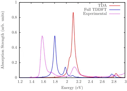
FIG. 3: Absorption spectrum of bacteriochlorophyll in implicit solvent as calculated with both the TDA and full TDDFT in comparison to experimental data of bacteriochlorophyll in toluene. A Lorentzian broadening of 0.025 eV is used for the TDDFT results and the experimental data is scaled such that the peak height of the Qy transition agrees with that of the Qy peak obtained from full TDDFT.

how the input structure was obtained from X-ray diffraction results), optimise the atomic

positions in vacuum and then calculate the TDA and full TDDFT spectra of the system

within an implicit solvent model[48], where the static dielectric function ϵ is chosen to be

2.38 in order to match the dielectric function of toluene at room temperature. The final

structure of BChl ain vacuum can be found in Fig. 2. As can be seen, the porphine ring is

entirely flat in this configuration, while the alkane tail folds underneath the ring structure.

The results of the TDDFT calculation as compared with the experimental results[53] can

be found in Fig. 3. As can be seen the experimental spectrum shows three main features: A

main absorption peak at around 1.6 eV, a shoulder between 1.65 and 1.75 eV and a second

peak at around 2.1 eV. The first and second peaks are commonly referred to as the Qy

and Qx transitions respectively and can be characterised as HOMO→LUMO and

HOMO-1→LUMO transitions in a single-particle picture. As can be seen from Fig. 3, the TDA

results generate only a single main peak at 2.12 eV that is of Qy character. This main peak

shows a shoulder at 2.05 eV that is mainly of HOMO-1→LUMO and HOMO-2→LUMO

character. The full TDDFT spectrum on the other hand produces a Qy peak at 1.80 eV

that is the lowest excitation of the system, as well as a second peak of Qx character at

1.98 eV, but fails to reproduce a shoulder to the Qy peak. It also shows a third peak with

It can therefore be concluded that the TDA fails in correctly reproducing the absorption

spectrum of BChl a in toluene. Not only is the Qy transition overestimated by 0.47 eV

compared to the experimental results, it does not correspond to the lowest excitation of the

system and there is no clean Qx transition. The full TDDFT results show a considerable

improvement. While the Qy transition is still overestimated by 0.2 eV, it now corresponds

to the lowest excitation of the system and there is a considerable splitting between the Qy

and Qx transitions. However, the full TDDFT results underestimate the energy of the Qx

transition by around 0.14 eV compared to experimental results and fail to exhibit a shoulder

to the Qy transition.

The origin of some of the failures of the TDA can be traced by breaking down the

excitations into individual Kohn-Sham transitions. In full TDDFT, the Qy transition is

almost exclusively (to 95%, as compared to 60% in the TDA) a transition between the

HOMO and the LUMO. In Bacteriochlorophyll, this transition has a strong dipole moment

associated with it, which in turn causes V{_SCF1} to be large and the TDDFT energy to show a large increase compared to the HOMO-LUMO energy difference. In full TDDFT, this

large dipole is screened by the de-excitation vector Y which is almost entirely made up of

the same HOMO-LUMO transition, thus significantly lowering both the excitation energy

and the oscillator strength. In the TDA, Y = 0 and instead the large dipole moment of

the HOMO-LUMO transition is screened by mixing in smaller fractions of higher energy

transitions, including fractions of Qx transition. This causes the Qy transition to have a

significantly higher energy and larger oscillator strength in the TDA and also contributes to

the absence of a clean Qx transition.

Since optimising the atomic positions of BChlain vacuum might have lead to a structure

that is unrealistic for the system solvated in toluene, it is not clear how much of the failure

of full TDDFT to reproduce the experimental results is due to the choice of

exchange-correlation functional used in this work. In order to obtain a more realistic structure of

BChl a in toluene, we make use of the classical molecular dynamics package AMBER[49].

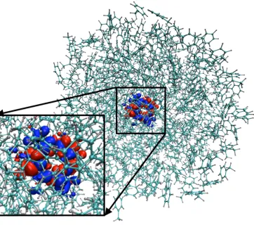
We solvate BChla in 704 molecules of toluene (corresponding to 10,700 atoms for the total

system) and equilibrate the system to 300 K and a pressure of 1 atm, followed by a 300 ps

simulation in the NVE ensemble. From this MD run we take 8 snapshots 10 ps apart that

are then used as input atomic positions in the TDDFT calculations. In order to include

0 0.1 0.2 0.3 0.4 0.5 0.6 0.7 0.8

1.2 1.4 1.6 1.8 2 2.2 2.4 2.6 2.8 3

A

b

so

rp

ti

on

st

re

n

gt

h

(a

rb

.

u

n

it

s)

Energy (eV)

TDA Full TDDFT Experimental

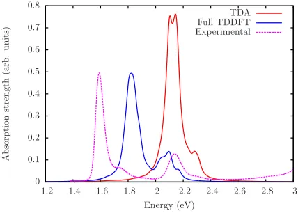
FIG. 4: Absorption spectrum of bacteriochlorophyll a in 15 ˚A of toluene as calculated on 8 MD snapshots with both the TDA and full TDDFT in comparison to experimental data of bacteri-ochlorophyllain toluene. A Lorentzian broadening of 0.025 eV is used for the TDDFT results and the experimental data is scaled such that the peak height of the Qy transition agrees with that of the Qy peak obtained from full TDDFT.

within a 15 ˚A radius from the Mg atom in the calculation, while representing the rest of

the solvent by an implicit solvation model. This process yields a system size of 700-800

atoms depending on the snapshot, which is closer to the limit of sizes that can be treated

by conventional O(N3) methods. The structure of the BChla molecule as obtained from a single MD snapshot can be found in Fig. 2. As can be seen, the alkane tail extends away

from the porphine ring in this configuration, while the ring itself is no longer perfectly flat.

The averaged full TDDFT and TDA spectra of the solvated MD snapshots as compared

with the same experimental dataset are shown in Fig. 4. Note that the full TDDFT results

now show the Qy transition at 1.83 eV and the Qx transition at 2.10 eV. While the Qy

transition is still overestimated by 0.2 eV, the shape of the feature is considerably improved,

as the Qx transition is now in very good agreement with experimental results, both in its

positioning and in its intensity. It is worth pointing out that a number of snapshots also

show a shoulder to the main Qy transition that is of HOMO-2→LUMO character. However,

in the averaged spectrum this feature is not as pronounced as in the experimental spectrum,

which can be due to the fact that the splitting between the Qx and Qy transitions is too

small compared to experiment. The TDA results on the other hand still fail to reproduce

0 0.1 0.2 0.3 0.4 0.5 0.6

1.2 1.4 1.6 1.8 2 2.2 2.4 2.6 2.8 3

A

b

so

rp

ti

on

st

re

n

gt

h

(a

rb

.

u

n

it

s)

Energy (eV)

Full TDDFT explicit solvent Full TDDFT implicit solvent Experimental

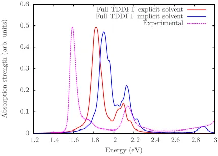
FIG. 5: Comparison between the full TDDFT spectrum of bacteriochlorophyll in 15 ˚A of toluene, averaged over 8 snapshots, and the averaged spectrum from 8 implicit solvent calculations using the same atomic positions for the bacteriochlorophylls. A Lorentzian broadening of 0.025 eV is used for the TDDFT results. Both spectra are plotted against experimental data that is scaled such that the peak height of the Qy transition agrees with that of the Qy peak obtained from full TDDFT in explicit toluene.

present in Fig. 3 has disappeared. The spectrum shows a new peak at approximately 2.3 eV

that does however have a different character to the Qx transition in full TDDFT. A clearly

identifiable Qx transition is still absent from the TDA results. It can therefore be summarised

that full TDDFT yields a much improved representation of the experimental results at the

PBE level as long as a realistic structure for the solute and the solvent environment is

obtained. The main failure of full TDDFT for this system is the overestimation of the Qy

transition by 0.2 eV which can most likely be ascribed to errors in the exchange-correlation

functional used.

While the 700-800 atom systems obtained from classical MD yield a relatively good

spec-tral shape for full TDDFT at the PBE level, they are considerably larger than the 140 atoms

of the solute alone. It is therefore worth investigating how much of the improvement of the

spectrum from Fig. 3 to Fig. 4 is due to the different ionic positions of the solute and how

much is due to an explicit quantum mechanical treatment of solvent molecules in the

calcu-lation. For this purpose we take the atomic positions of BChl a from the 8 MD snapshots

and compute the absorption spectrum in implicit solvent, without including any explicit

0 500 1000 1500 2000

0 1000 2000 3000 4000 5000 6000 7000 8000

T

im

e

(s

)

Number of atoms Linear-response operator

V{_SCF1}

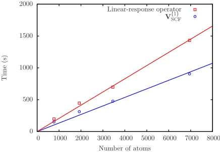
FIG. 6: Time taken for applying the TDDFT operator and calculating V{_SCF1} for different sys-tem sizes of bacteriochlorophyll a in toluene. The lines shown are linear fits. Calculations were performed on eight SandyBridge nodes containing 16 cores each.

the positioning of the Qx transition in implicit solvent is in very good agreement with the

experimental data. However, its oscillator strength is significantly overestimated.

Further-more, the explicit solvent environment causes the Qy transition to red-shift by about 0.1 eV.

It can be concluded that while most of the improvements in spectral features compared to

Fig. 3 are due to the more realistic atomic positions of the Bacteriochlorophyll in toluene,

the explicit inclusion of the toluene environment at the TDDFT level yields a spectrum that

is in closest agreement with experimental results.

In conclusion it can be summarised that full TDDFT at the PBE level reproduces

ex-perimental results to a satisfactory degree, while the TDA completely fails in this system.

The best agreement between experiment and calculation is obtained when taking the atomic

positions of an MD snapshot of BChl in toluene and including the local solvent environment

explicitly in the TDDFT calculation. While an explicit treatment of the solvent molecules

requires large scale TDDFT calculations, it is demonstrated that the method presented in

this work is well suited for tackling these systems, opening up the possibility of more detailed

studies of solvent effects on chromophores.

C. Linear-scaling capabilities

We now focus on demonstrating the linear-scaling capabilities of the TDDFT method