warwick.ac.uk/lib-publications
Original citation:
Dinh, Truong, Ahn, Kyoung Kwan and Marco, James. (2016) A novel robust predictive control
system over imperfect networks. IEEE Transactions on Industrial Electronics .
doi: 10.1109/TIE.2016.2580124
Permanent WRAP URL:
http://wrap.warwick.ac.uk/81425
Copyright and reuse:
The Warwick Research Archive Portal (WRAP) makes this work by researchers of the
University of Warwick available open access under the following conditions. Copyright ©
and all moral rights to the version of the paper presented here belong to the individual
author(s) and/or other copyright owners. To the extent reasonable and practicable the
material made available in WRAP has been checked for eligibility before being made
available.
Copies of full items can be used for personal research or study, educational, or not-for profit
purposes without prior permission or charge. Provided that the authors, title and full
bibliographic details are credited, a hyperlink and/or URL is given for the original metadata
page and the content is not changed in any way.
Publisher’s statement:
© 2016 IEEE. Personal use of this material is permitted. Permission from IEEE must be
obtained for all other uses, in any current or future media, including reprinting
/republishing this material for advertising or promotional purposes, creating new collective
works, for resale or redistribution to servers or lists, or reuse of any copyrighted component
of this work in other works.
A note on versions:
The version presented here may differ from the published version or, version of record, if
you wish to cite this item you are advised to consult the publisher’s version. Please see the
‘permanent WRAP url’ above for details on accessing the published version and note that
access may require a subscription.
Manuscript received November 29, 2015; revised March 05, 2016; accepted April 15, 2016. This work was supported by the 2017 Research Fund of the University of Ulsan.
T. Q. Dinh and J. Marco are with the Warwick Manufacturing Group (WMG), University of Warwick, Coventry, UK (e-mail: [email protected]; [email protected]).
K. K. Ahn is with the School of Mechanical Engineering, University of Ulsan, Namgu Muger2dong, Ulsan 680-749, Korea (corresponding author to provide phone: 82-52-259-2282; fax: 82-52-259-1680; e-mail: [email protected]).
Abstract—This paper aims to study on feedback control for a networked system with both uncertain delays, packet dropouts and disturbances. Here, a so-called robust predictive control (RPC) approach is designed as follows: 1- delays and packet dropouts are accurately detected online by a network problem detector (NPD); 2- a so-called PI-based neural network grey model (PINNGM) is developed in a general form for a capable of forecasting accurately in advance the network problems and the effects of disturbances on the system performance; 3- using the PINNGM outputs, a small adaptive buffer (SAB) is optimally generated on the remote side to deal with the large delays and/or packet dropouts and, therefore, simplify the control design; 4- based on the PINNGM and SAB, an adaptive sampling-based integral state feedback controller (ASISFC) is simply constructed to compensate the small delays and disturbances. Thus, the steady-state control performance is achieved with fast response, high adaptability and robustness. Case studies are finally provided to evaluate the effectiveness of the proposed approach.
Index Terms—Networked control system, time delay, state feedback control, predictor, neural network, buffer.
I. INTRODUCTION
ETWORKED control systems (NCSs) are spatially distributed systems, in which actuators and sensors at the plant side are connected to a controller at the remote side. Due to having many advantages over the traditional control schemes via point-to-point wiring, NCSs have been deploying worldwide in various applications, such as power grids, transportation systems, teleoperation or remote systems.
However for practical uses of NCSs, the most important issues are network-included random time-varying delays and packet dropouts which deteriorate the control performances and, easily cause the instability [1], [5], [25], and [29]. Generally, time delays can be classified into three components: computation delays at the controller and communication delays at the forward and backward channels.
Many studies in literature addressed stability of NCSs with delay problem only [1]-[6]. Here, the controller designs were
depended on the assumptions in which the time delay was constant [1], bounded [2]-[5] or had a probability distribution function [6]. Other researchers focused on analyzing time delay problem at communication channels to evaluate its effects on the system performances as well as to compensate these undesirable effects [7] and [8]. For NCSs with large delays, a new control concept based on variable sampling periods using neural network or prediction theories has been recently adopted [9]-[11]. Nevertheless, the observation of real delay data to train and construct the NCSs was not appropriately discussed in these studies. To solve this problem, an advanced variable sampling period control concept has been developed for systems containing random delays [29]. The effectiveness of this concept in accurately detecting and predicting the delays without requiring a training process was proved through real-time experiments.
To adapt NCSs to not only time delays but also packet dropouts, many important methodologies, such as predictive control [12]-[16], adaptive control [17], [18], hybrid control [18], and robust control [19]-[26], were proposed. In an early study with unknown networked systems [18], the randomly missing output feature was considered and modelled as a Bernoulli process and the Kalman filter-based adaptive control scheme was successfully conducted to estimate both the missing output measurements and system parameters. For systems with network problems existing on both the forward and backward channels, Markov chains were employed to model the delays and packet dropouts and, subsequently, incorporated into the well-known two-mode-dependent state feedback controller in the general and practical way [20]. The robust stability of this control method was significantly improved through the implementation of the H2 and H∞ norms to perform the robust H2 and robust mixed H2/H∞ two-mode-dependent controller [21], [22]. Several studies also developed the robust controllers based on the other advanced concepts, in which the network delays are presented in the general form and bounded by both upper and lower limits to reduce the conservatism problem [23]-[25]. Or, the integral action was used to compensate the nonzero disturbance issue [25]. By using these techniques, the NCS performances were remarkably improved over the traditional methods. However in most studies, delays and packet dropouts were assumed to be priorly known and bounded to design the controllers. The complex control designs to deal with both the communication problems and disturbances also restrict their applicability. Another trend to improve networked control performances is known as control based on efficient networks with adaptive
A Novel Robust Predictive Control System
over Imperfect Networks
Truong. Q. Dinh,
Kyoung. K. Ahn,
Member, IEEE
and
James Marco
buffers [27] or with a compensation strategy [28]. Although these methods could achieved good control results, the applicability may be limited because of the complex network designs. Furthermore, the uses of fixed sampling period and dynamic buffers with large sizes at both channels could limit the control performances. Additionally, delays due to a complex computation of a control system is another important factor affecting directly on the performance, especially in NCSs [29]. Recently, a robust control approach named RVSPC [36] developed from [29] has been proposed as a feasible solution to address all of these problems. Its controllability has been clearly proven through both simulations and real-time experiments. Although the results are remarkable, the RVSPC still remains some open problems:
The robust state feedback control module is basically designed for a linear NCS of which the system state is clearly known. It is actually not easy to be achieved in practical applications where most of system states are time-variant. In addition, disturbance cancelation are not considered in this control module design;
With the use of ZOH for updating instants, the control performance may be degraded or even, unstable when existing long delays and/or high packet loss rate on the communication channels;
The role of grey model-based prediction is limited to only switch between the control modules and to vary the sampling period.
In order to overcome these drawbacks as well as to improve the control quality, this study aims to develop a novel robust predictor control (RPC) approach based on the advantages of the previous studies, [29] and [36], to deal with networked systems included both of three delay components and packet dropouts. The merit of the RPC can be expressed as bellows: 1- Different from [36], and other studies on network analysis, delays and packet dropouts are quickly and accurately detected online by a network problem detector (NPD) using a new rule to detect network problems.
2- Developed from [29] and [36], a so-called PI-based neural network grey model (PINNGM) is robustly constructed in a general form for a capable of forecasting precisely in advance the network problems and impacts of disturbances on the system response.
3- Using the NPD and PINNGM, a hybrid time-event-driven scheme is derived to avoid long delays during the communication.
4- Different from other networked control techniques normally using ZOH or larger buffers, a small adaptive buffer (SAB), of which the buffer size is online optimized based on the PINNGM, is generated on the plant side to compensate packet dropouts on the forward link.
5- By using the PINNGM and SAB, an adaptive sampling-based integral state feedback controller (ASISFC) is built with four advanced characteristics:
- To compensate packet dropouts on the forward channel, sk-step-ahead control technique is suggested to combine with
the SAB to produce the control input in time;
- To compensate packet dropouts on the backward channel, a state observer is employed;
- To compensate the estimated influences of disturbances, an integral term is added to the state feedback control algorithm; - To avoid the conservatism as well as to save the computational time in producing the control input online, a set of the control gains is pre-derived for a set of system states with small delay regions and then, stored in a look-up table.
As a result, the steady-state control performance is guaranteed with high adaptability and robustness. The rest of this paper is organized as follows. Section II introduces the concerned problem. The RPC architecture is shown in Section III. The design procedures for the PINNGM and ASISFC are presented in Section IV and Section V, respectively. Experiments are provided and discussed in Section VI. Finally, we conclude the paper in Section VII.
II. PROBLEM DESCRIPTION
A generic system without delays can be described as:
( 1) ( ) ( )
( 1) ( )
x k Ax k Bu k
y k Cx k
(1)
where x k( )xkRmx, ( )u k ukRmuand ( )y k ykRmy
denote the state vector, control input and system output, respectively; A, B and C are known matrices. Without loss of generality, the reference r(k) is assumed to be zero.
Remark 1: The RPC scheme is developed for system (1) over an imperfect network with following issues:
ca, sc, andcomin turn denote communication delays on forward and backward channels, and computation delay. The computation delay can be bounded, com com
k
. Two
threshold values,caandsc, are used to classify delays in which large delays are treated as packet dropouts:
1
or Smalldelay
or Packet dropout
= + ;
ca ca sc sc
k k
ca ca sc sc
k k
sc com ca
k k k k
(2)
“Virtual” switches, Sca and Ssc, in turn represent the packet
dropouts in the forward and backward channels: Skca (or
sc k
S ) is opened (=1) when a packet loss event exists;
and
ca sc
k k
p p denote the numbers of continuous packet dropouts on forward and backward channels up to step kth. The sensors are time-driven with a variable sampling period
Tk. This period is online regulated in advance to ensure that
it covers the total system delay in (2), k Tk;
The controller and actuators are hybrid time-event-driven. They are event-driven if the delays satisfy (2); otherwise, they are time-driven to avoid the packet dropout problem.
III. ROBUST PREDICTIVE CONTROL APPROACH
actuators and n sensors) using the RPC and, other execution tasks which cause unavoidable computation delays. The RPC mainly consists of five modules: NPD detector, PINNGM-based predictor, variable sampling period adjuster (VSPA), SAB buffer and ASISFC controller.
A. NPD Detector
The NPD is to detect online accurately both the time delays and packet dropouts based on (2) and then, to support these information to the other control modules.
Remark 2: using the same hardware and logics developed in [36], the NPD employs the PIC18F4620 MCU (from Microchip) equipped with the 4-MHz oscillator and the embedded time stamp-based detection logic to manage the networked system. Thus, real-time measurement accuracy is 50s[36] and, the NDP outputs for each step are the delay set,{ kca, ksc, kcom}, and packet dropout set, { , }
ca sc
k k
p p .
Based on Remark 1, the controller and actuators are selected as time or event -driven according to the real-time measurement using the NDP and condition (2). Thus, it is possible to use a so-called hybrid period TC (or TA) to
represent the driven state of the controller (or actuators). From Remark 2, TC and TA can be derived as
1
min , min ,
min , min ,
;
C com ca ca sc sc d
k k k k
A sc sc com ca ca d
k k k k
d com ca sc
T
T
(3)
B. PINNGM-Based Predictor
Grey model is known as a feasible solution for online prediction while requiring only a few historical data about the predicted object [29]-[36]. Although the AGM(1,1) proposed in [36] could overcome all drawbacks of typical grey models, it requires the fuzzy control knowledge from the user once employing this model for each specific application. In this study, a grey model is efficiently developed in a general form of first order – N variables and denoted as PINNGM(1,N).
Remark 3: The PINNGM is developed with following characteristics:
The model is able to forecast any random time-series data by using a simple data conversion with additive factors.
A recurrent signal is integrated as a model input to exhibit the dynamic temporal behavior.
The model consists of a main grey model, tagged as MGM(1,N), and a proportional-integral (PI) -based neural network weight tuner, tagged as PINNWT.
Lyapunov stability constrain is used to guarantee the robust prediction.
Network
T(k)
Desired Tasks
y(k) Disturbances
Plant Other Tasks
ASISFC (TC(k))
-+
ca
sc
d(k)
PINNGM
VSPA NDP
Sca
Sensor 1
Sensor n MCU
Ssc com
Dr(k+1)
Actuator 1
Actuator n SAB
(TA
(k),
BS(k))
TC (k)
TA(k)
BS(k)
T(k)
RPC-based Controller
y(k)
yD(k)
Fig. 1. A generic NCS architecture using proposed RPC approach.
As stated in the Introduction and from Fig. 1, the PINNGM(1,N) is employed with two main functions:
First, to perform sk-step-ahead prediction of the system
delays, { s, s, s}
com ca sa k i k i k i
, and packet dropouts,
ˆ
{ }, 1,...,s
s
ca
k i s k
p i where sk is defined as:
2
ˆ
min at which 0; 2,3,...
k
ca
k k i
s
s i p i
(4)
These predicted values are used to set the sampling period for the sensors and the size of the SAB buffer.
Second, to estimate the current system response (when existing a packet dropout on the backward channel) as well as the sk-step-ahead responses. This information is then fed
into the ASISFC to derive in advance the sk-step-ahead
control inputs to compensate the packet dropouts on the forward channels.
C. VSPA Adjuster
Based on Remark 1, it is necessary to regulate the sensors’ sampling period synchronously with the delays defined by (2). By considering the system process time constant as Tp, the
sampling period for a future step (k+is)th is defined based on
the PINNGM and a MAX-MIN rule as
0 0
0 1
0 0
, /
ˆ ˆ ˆ
max , min , min ,
0.1 , is initial sampling period
s
s s s
k i T T new
sc sc com ca ca new k i k i k i
p
T k T k T T
T T
T T T
(5)
where * is ceiling function to return nearest integer value. Meanwhile, the hybrid periods, TC (or TA), are estimated in
advanced in order to perform the sk-step-ahead control:
1
ˆ ˆ min ˆ , min ˆ ,
ˆ min ˆ , ˆ min ˆ ,
C com ca ca sc sc d
k k k k
A sc sc com ca ca d
k k k k
T
T
(6)
D. SAB Buffer
To eliminate forward packet dropout effect, the SAB is only utilized at the plant side. Selection of the buffer size (BS) affects directly on the control performance. With the ZOH, the controlled system is difficult to follow the desired goal when there is a large number of forward packet dropouts. On the contrary, the control performance becomes poor when using a large size buffer (designed for the worst network state). Thus, the key principle here is to optimize online the buffer size SB based on the PINNGM to store enough commands to drive the
actuators during eachpkcacontinuous forward packet dropouts.
For each working step, the commands for actuators are then extracted from the SAB following the first-in-first-out rule.
The procedure to tune the SAB size can be described as: Initial step: Define the minimum size of the SAB, BSmin. In
this case, it is selected as, BSmin = min(sk)= 2. Then, set the
initial size of the SAB: BS0 = BSmin.
Step 1: For each step (k+1)th at the controller side, based on
Generate a set of time-stamped control inputs,{uk1,...,uk sk}using the ASISFC.
Step 2: For each step (k+1)th at the plant side: If a new package sent from the controller is arrived:
+ Re-size the SAB with the new size BSk+1.
+ Update the new control inputs and store in the SAB.
Extract data from the SAB to drive the actuators based on the first-in-first-out principle.
E. ASISFC controller
The ASISFC takes part in driving the actuators to reach the desired target. As mentioned above, the packet dropout problem is compensated by the use of NDP, PINNGM and SAB with sk-step-ahead control technique. Thus, the ASISFC
is designed to address only the small delays defined by (2) with following characteristics:
The state feedback control algorithm is used to generate the main control input;
An integral term is added to the control algorithm to compensate the bad effects of disturbances.
A state observer is implemented to adapt to the time variant system states.
Based on the threshold values of small delays, a set of the control gains is pre-derived for a set of system states with small delay regions and stored in a look-up table.
IV. PINNGM-BASED PREDICTOR
A. Main Grey Model MGM(1,N)
This section is to generate a grey model between N relevant objects (or characteristics),
1 2
{ , ,..., }
N
obj obj obj
y y y , of a system.
Without loss of generality, object 1st is assumed to be the object which needs to be estimated based on a historical data set of the relevant objects. The procedure to predict this object using the MGM(1,N) can be designed with following steps: Step 1: Prepare an input grey sequence for each object obji: Update the data sequence with the newest values:
yobji(tO1),yobji(tO2),...,yobji(tOm) ;
i1,...,N m; 5. (7) Define corresponding raw input grey sequences as
0
0 0 0
1 2
( ), ( ),..., ( ) ; 1,..., ; 5.
i i i i
raw raw raw raw n
y y t y t y t i N n (8)
Define a data distribution checking condition:
1
1 1 1
/ 2; ; 2,...,
; : previous time stamp of ;
i
Oi MGM Oi Oi O i
O O Olast Olast obj O
t T t t t i m
t t t t y t
(9)
here TMGM is the desired prediction sampling period;
If (9) is satisfied, then update directly sequence (8) as the (7); Otherwise, sequence (8) is created as sequence (10) with approximately equal time intervals based on sequence (7) and the spline function, SP, introduced in [36]:
0 0
1 1 1
1
; ; ;
1,..., ; 2,..., ; / ; j 1,..., 1;
i i i
raw obj O raw k k Oj Oj k O j Om O MGM
y t y t y t SP t t t t t
i N k n n t t T m
(10)
here * is floor function to return nearest integer value.
To exhibit the dynamic temporal behavior of the model, a
recurrent signal as the current-step predicted value of the
predicted object,
10
ˆraw n
y t , is generated and added to its
sequencey raw0
tn to become:
1 1 1 1
0 0 0 0
1 , 2 ,...,ˆ ; 5.
raw raw raw raw n
Y y t y t y t n (11)
Remark 4: By adding two non-negative factors c1 and c2 derived by Theorem 1 in [36], sequence (11) satisfies the two checking conditions of a grey model: positive sequence and quasi-smooth – quasi-exponential law checking condition.
Generated a grey sequence (12) using Remark 4:
1
0 0 0 0
1 2
0 0
1 2
, ,..., 0; 5
; 1,..., .
n k raw k
y y t y t y t n
y t Y t c c k n
(12)
Step 2: Generate a new series y(1) by generating from y(0):
1 0 1 1 2 1, 1, 2,...,
.
k
i i i
k
raw i i i
y k y t t k n
Y t c c t
(13)Step 3: Create the background series z(1) from y(1) as
1
1 1
2 1
1 ; 2,...,
k k k k k
z t w y t w y t k n (14)
where
1, 2
k k
w w is a weight factor set which is designed as
1
1 1 2 1 2
2
1 1 2 1 2
0.5 1 1 1
0.5 1 1 1
PINN PINN
k k k
PINN PINN
k k k
w w w
w w w
(15)
where 0wkPINN 1 is derived using the PINNWT tuner;
1 2
{ , } is a set of activated factors and defined as
1 1 1
1 1 1
0 0
1 1
0 0
1 2 1 1
{1,0}, IF : ;
{ , } {1,1}, IF : ;
{0,1},Others.
raw k k raw k obj k raw k obj k raw k k
y t SP t y t y t
y t y t y t SP t
(16)
Step 4: Establish the grey differential equation
0
1
3 1 3
2
1 .
i
N
k k i raw k i
y t az t b b y t
(17)where3is an activated factor which is enabled (or 1) when N=1, and vice versa.
By employing the least square estimation ([30],[36]), one has:
1 1
ˆ ˆ
ˆ ˆ T ( )
T T ab a b bN B B B Y
(18)
where
2 2 12 3 3 2 3 2
1
3 3 3
0 0 0
2 3 1 1 , 1 1 . N N raw raw
n raw n raw n T
n
z t y t y t
B
z t y t y t
Y y t y t y t
Step 5: The MGM(1,N) prediction is then setup as:
1
1 23 1 3 1
0 2
1
ˆ 1 ˆ ˆ
ˆ .
ˆ 1
i
N
i raw k k k k i
k
k k
b b y t a w w y t
y t
w a t
(19)of 1
obj
y at step (k+pk)th can be computed as
1 0 0 1 2 ˆ ˆ k kraw k p k p
y t y t c c (20)
where pk is the step size of the grey predictor.
B. PINNWT Tuner and MGM(1,N) Stability Analysis
By considering the prediction of 1
obj
y using the MGM(1,N)
as a tracking control problem with the control input is PINN k
w (in
(15)), it is possible to derive a robust controller to enhance the robust prediction of this model. Here based on Remark 3, the PINNWT controller is designed with a Lyapunov stability condition to regulate the ‘control input’ PINN
k
w .
Here, the PINNWT consists of three layers: an input layer as a prediction error sequence MGM { ,...,1 n1}
k k k
e e e ,
0
ˆ 0
i
k raw i raw i
e y t y t , a hidden layer with two nodes, P and I,
following PI algorithm, and an output layer to compute the weight factor, PINN
k
w . Define { Pi, Ii}
k k
w w is a weight vector of the
hidden nodes with respect to input ith, and { P, I} k k
w w is the
weight vector of the output layer. Therefore, the output from each hidden node is derived based on PI algorithm:
1 1
1
1 1
: Node P
: Node I
n P Pi i k i k k n I I Ii i k k i k k
O w e
O O w e
(21)Then, the output from the network or the control input for ‘plant’ MGM is obtained using sigmoid activation function:
11 OkNN ,
PINN NN NN P P I I k k k k k k k
w f O e O w O w O
(22)
In order to ensure the robust prediction, the back-propagation algorithm based on the Lyapunov stability condition is used to tune the PINNWT. Define a prediction error function as
1 1
2 2
1 0 0 1
1 ˆ 1
0.5 n 0.5 n .
MGM i
k i raw i raw i i k
E y t y t e
(23)Thus, the weight factors of the PINNWT are online tuned for each step, (k+1)th, as follows:
/ / / / 1 / / / / 1 / /
P I P I P I MGM P I k k k k k Pi Ii Pi Ii Pi Ii MGM Pi Ii k k k k k
w w E w
w w E w
(24)
where / /
,
P I Pi Ii k k
are learning rates within range [0,1]; the other factors in (24) are derived using the partial derivative of the error function (23) with respect to each decisive parameter and chain rule method [37].
Theorem 1: By selecting properly the learning rates Pi Ii/ P I/
k k k
for step (k+1)th to satisfy (25), then the
stability of the PINNGM prediction is guaranteed.
1 2
1 0.5 0
n i
k k k k i e F F
(25) with 1 1 .j MGM j MGM n
k k k k k Pi Pj Ii Ij
j k k k k
e E e E
F
w w w w
Proof: Define a Lyapunov function as
2
21 0 0 1
1 ˆ 1
0.5 n 0.5 n .
MGM i
k i raw i raw i i k
V y t y t e
(26)The change of this Lyapunov function is derived as
2 2 11 1 1
2 1
1 1
0.5
0.5 , .
n
MGM i i k i k k
n i i i i i i k k k k k k i
V e e
e e e e e e
(27)From the PINNWT structure, one has:
1 1
.
i i n
i k Pj k Ij k Pj k Ij k
j k k
e e
e w w
w w
(28)The termswkPj,wkIj are from (24). By using the partial derivative and selecting Pj Ij/ P I/
k k k
, (28) becomes: .
i k k k
e F
(29)
From (29), (27) is rewritten as
1 2
1 1 0.5 .
n MGM i
k i k k k k
V e F F
(30)The MGM(1,1) prediction is guaranteed to be stable only if
1 0,
MGM k
V k
. It is clear that exceptk, the other factors in (30) can be determined online based on the prediction error and the chain rule method [37]. Hence for each working step, it is easy to select a proper value ofkto make (25) satisfy. Therefore, the proof is completed.
C. PINNGM(1,N) Application to RPC and Examples
As presented in Section III.B, the PINNGM model is utilized for the RPC design as:
To perform sk-step-ahead prediction of the system
delays/packet dropout, PINNGM(1,1) is employed, in which the model input is a vector of historical delays/packet dropouts;
To perform sk-step-ahead prediction of the system response,
PINNGM(1,2) is chosen, in which the model inputs are the historical data of system response and control input. This is because the system response is relevant to the control input. The applicability of the PINNGM models is investigated via the following examples.
Example 3.1: A comparative study of four grey models, GM(1,1), SAUIGM(1,1) [29], AGM(1,1) [36] and PINNGM(1,1), has been carried out to investigate the capability in predicting the network delay problem studied in [29] and [36]. Because the GM is limited to equal-time-series prediction, the real-time estimations were performed for a 30-second period in which there were only time delays in the network. The delays were observed by the NPD with a fixed sampling rate of 10ms [29]. The one-step-ahead estimation results were obtained and analyzed in Table I using three evaluation criteria: average relative error (ARE), root mean square error (RMSE) and coefficient of determination (R2).
in Table I. However, the fuzzy inference of the AGM may need to be re-designed once changing the application or prediction step size. This is investigated through the second example.
Example 3.2: Series of delay predictions using the four grey models in Example 3.1 have been done with different prediction step sizes (varied from 1 to 30) to evaluate the sk-step-ahead prediction ability. The comparison result is then
displayed in Fig. 2. Here, the GM prediction accuracy was totally reduced according to the step size increase. Although the SAUIGM could improve the accuracy, its fitness was not kept stably. Only with the AGM and PINNGM which were optimized by the robust conditions, the precise estimations were almost guaranteed. However, the performance of the PINNGM was better than that of the AGM due to the adaptability of the neural network, PINNWT, over the change of prediction step sizes.
V. ASISFC CONTROLLER DESIGN
A. ASISFC-based NCS Analysis
As described in the Introduction, Remark 1 and Section III, the ASISFC controller is designed to create the sk-step-ahead
control inputs for networked system (1) with only small delays defined in (2). Without loss of generative, the followings are to design the control gains for the networked system (1) only at step (k+1)th which can be simplified to the following
delayed system:
1 2
2 1 1 1 1 1
k k k k k k k
x Ax Bu Bu (31)
where the matrices in (31) are derived from (3) and (5):
1 1 1 1 1 1 1 2
1 1 1
0 , , ; A k k k k A k k
T T T
AT At At
k k k
T T
A e B e Bdt B e Bdt
(with step (k+is)th (is =2,…,sk), 1and 1
A A k k
T T in (31) are replaced
by ˆk iA andˆk iA
s s
T T ).
From (3), 1
A d k
T , and Section III.E, it is possible to
consider the control design for system (31) similarly as for a set of system with D small delay regions having the same intervals:
TABLEI
REAL-TIME ONE-STEP-AHEAD DELAY PREDICTIONS
Evaluation criteria
Prediction models
GM SAUIGM AGM PINNGM
ARE (%) 8.6720 0.9664 0.5271 0.4783
RMSE (10-4) 28.4937 3.7635 2.026 1.8398
R2 0.8818 0.9679 0.9822 0.9891
5 10 15 20 25 30
60 70 80 90 100 GM Model SAUIGM Model AGM Model PINNGM Model M od el F itn es s [ % ]
Prediction Horizon [step]
Fig. 2. Delay prediction model fitness vs. prediction step size sk.
4
1 2
2 1 1 1 1 1
1 D
i i i
k k k k k k k
i
x A x B u B u
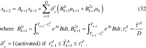
(32)where 1 1
1 1 2 1 1 0 , , d i k k d i k d T T
i At i At d
k k i
T
B e Bdt B e Bdt
D
;4 1 1
ˆ 1(activated) if
i d A d
i Tk i
.
To ensure a robust tracking performance with disturbance attenuation, the control rule for system (32) is designed as a state feedback gain combine with an integral gain:
1 2
1 1 1
d
k k k
u K x K x (33)
where K1Rmu mx andK2Rmu md are the desired control gain matrices;xkd1Rmdis the disturbance integration factor:
2 1 1 1 1
d d d
k k k k k
x x y r x Cx (34)
Replacing (33) and (34) in to (32), one has:
4 4
4
1 1 2 1 2
2 1 1 1 1
1 1
1 2 2
1 1 1
1
D D
i i i i
k k k k k k
i i
D
i i i d
k k k
i
x A B K x B K K C x
B B K x
(35) or:2 1 1
k k k
X X (36)
where,
1 11 12 13
1 1
1
; 0 0 ;
0
k
k k k
d k
x
X x I
C I x
4 4 41 1 2 2
11 1 1 1
1
2 1 1 2 2
12 1 13 1 1
1 1
,
, D
i i i
k k k
i
D D
i i i i i
k k k
i i
A B K B K C
B K B B K
To adapt to the time-variation of the system state, a state observer is implemented into system (32):
4
1 2
2 1 1 1 1 1 1 1
1
ˆ ˆ ˆ
D
i i i
k k k k k k k k k
i
x Ax Bu Bu L y y
(37)where xˆk1Rmx,yˆk1RmyandLRmx myx denote the
estimated state, estimated system output and observer gain, respectively. The state estimation error is ek1xk1xˆk1.
The packet dropouts on the backward channel can be compensated by the PINNGM(1,2) (Section IV.C) to estimate
the system response (denoted asyˆM). Thus, system (37) can be re-written in a general form as
4
1 2
2 1 1 1 1 1 1 1
1
ˆ ˆ ˆ
D
i i i
k k k k k k k k k
i
x Ax Bu Bu L y y
(38)
1 , 0
1
ˆ 1 , 1
sc k
M sc
k
y k if S
y k
y k if S
(39)
[image:7.612.314.562.55.138.2] [image:7.612.46.296.555.723.2]represented as
1
2 1
0 0
0 0
0 0 0
k
k k
A LC
E I E
(40)
or
2 1 1
E
k k k
E E (41)
where,
1
1
0 0
0 0 .
0 0 0
k E k
A LC
I
By combining (36) and (41), the closed-loop NCS using both state feedback control gain, disturbance integration gain and observer gain is expressed by
2 1 1 1
k k k k
X X LCE (42)
B. ASISFC Control Gain Design and Stability Analysis Theorem 2 [25]: Separation principle – If there exit two positive matrices, P and PE, such that:
1 1 0
T
kP k P
(43)
and,
1 1
(Ek )TPEkE PE0 (44)
hold, then the closed-loop NCS (42) is asymptotically stable. Proof: The proof of this theorem is addressed in [25]. Based on Theorem 3, the control gain design for system (42) is now simplified to the control gain designs for system (36) and system (41).
Theorem 3: If there exists a positive definite matrixP0, such that (43) hold, then the NCS (36) is asymptotically stable.
Proof: Select the following Lyapunov function:
1 1 1 1 1.
T
k k k k k
V X V X PX (45)
Using (36), the derivative of this function is obtained as
1 2 1 2 2 1 1
1 1 1 1.
T T
k k k k k k k
T T
k k k k
V V V X PX X PX
X P P X
(46)
Due to P>0, it is clear that Vk10if (43) holds, thus the
system (36) is asymptotically stable, the proof is completed. The sufficient condition for designing the controller is pointed out by Theorem 3. However when designing the control gains, the inequalities (43) may do not has the form of LMIs. In order to design the control gains, Theorem 4 is therefore introduced:
Theorem 4: If there exists a positive definite matrixP0, such that the inequalities:
1
1
0
T k
k
P
Q
(47)
hold with PQ = I, then the NCS (36) is asymptotically stable. Proof: Applying the Schur complement [38] to the equalities (43), one has:
1 1 1
0.
T k
k
P
P
(48)
LettingP1Q, (48) becomes (47). The proof is finished. Using Theorem 4 and the cone complementary linearization algorithm [39], the control gains can be solved by the following minimization problem involving LMI conditions:
minimizesubject to (47), 0, 0. trace PQ
P Q (49)
Remark 5: by applying Theorem 2, system (41) is asymptotically stable if existing a positive matrix PE which
satisfies (44). Thus in this case, the stability of system (41) can be guaranteed by design the observer gain L in order to placing all eigenvalues of the characteristic (Ak+1-LC) inside
the unit circle. This can be done easily by pole placement method [40].
Finally, the ASISFC control procedure for a NCS can be summarized as:
Step 1 – control gain preparation (off-line):
Divide the delay range dinto D small delay regions to input to (30);
Design a set of control gains K1 and K2 for system (36)
using Theorem 4 and (49);
Design a control gain L for system (41) using the pole placement method;
Generate a look-up table to store the designed control gains with respect to the set of delay regions.
Step 2 – sk-step-ahead control command generation (online): Based on the predicted system delays, select properly the
control gains from the gain look-up table;
Generate the sk-step-ahead driving commands with time
stamps and send to the SAB.
VI. CASE STUDY
This section considers a case study with speed tracking control of a networked DC servomotor system. The proposed RPC approach has been evaluated in a comparison with two controllers: the RVSPC developed in [36] and, the SSFC in [36] combined with a fixed buffer and the VSPA module, tagged as SSFC-FB.
A. System Configuration and Problem Investigation
Configuration of the networked DC servomotor system is presented in Fig. 3 and clearly described in [29] and [36]. The servomotor input-output transfer function can be expressed as
[image:8.612.318.564.622.730.2]
232300
.
0.001 20.93 493.4
p
G s
s s
The system can be also represented in the form of (1) with:
235870 4934200 1 0
, , .
1 0 0 32298000
T
A B C
Furthermore for the full evaluation, computation delays and two disturbance sources were applied to the system. The computation delays were observed from the control system of the real machine [36]. The first disturbance source came as the magnetic load applied to the motor shaft while the second source was simulated and added to the system feedback speed:
( ) Rand ( )N Nsin(2 N ) 1
N t t A f t
here AN was given randomly from 0.5 to 1; fN was varied from
1 to 5 Hz; RandN was a noise with power 0.005.
B. Control Parameter Setting
First, the RVSPC control gains were derived as presented in [36]. Second, based on the network condition, the SSFC-FB control gains were computed by considering the total delay as
0.1 . d
SSFC s
Then, the SSFC-FB control gain was found as
0.3652 0.2539
SSFC FBK while its buffer size was fixed
as 5. Third for the RPC design, based on Remark 1, the delay threshold values were selected as: com0.025 ,s
0.035 and 0.035
ca sc
s s
. The state feedback and integral control gains were, therefore, derived for a set of the total delay regions ranging from 0 to 0.095 with interval of 0.01s as shown in Table II. Meanwhile, the observer gain was derived as [1; 1.3217].
C. Experimental Results and Discussion
The real-time speed tracking control evaluation in the imperfect conditions, including both the three delays, packet dropouts, and disturbances, has been then performed using the comparative controllers. Here, the first disturbance source always applied to the motor shaft while the second disturbance source was only added to the feedback speed after 15 seconds.
Firstly, the experiments on the system without the simulated disturbances were done in which the desired motor speed was set as a constant of 10rad/s. The tracking results were then obtained as demonstrated in Fig. 4. The one-step-ahead delay prediction using the PINNGM was observed as in Fig. 5.
TABLEII
RPCCONTROL GAINS ACCORDING TO TOTAL DELAY
ˆA
T K1 K2
0~0.01 [0.2511 0.2001] 0.0038
0.01~0.02 [0.2587 0.2009] 0.0037 0.02~0.03 [0.2644 0.2037] 0.0037 0.03~0.04 [0.2723 0.2065] 0.0039 0.04~0.05 [0.2805 0.2086] 0.0038 0.05~0.06 [0.2869 0.2101] 0.0038 0.06~0.07 [0.3028 0.2152] 0.0039 0.07~0.08 [0.3213 0.2189] 0.0041 0.08~0.95 [0.3471 0.2234] 0.0040
In this case, the SSFC-FB controller could not ensure the smooth tracking result due to the use of fixed control gains and buffer, which were designed for the worst network conditions. Furthermore, the SSFC-FB lacked of the predictability of the system response, the controller could not derive the control inputs once there existed packet dropouts on the feedback channel. The tracking performance was significantly degraded when the packet dropout ratio increased and the second disturbance source was invoked into the system.
By using the RVSPC controller, the performance was improved by the advanced switching control based on the QFT and state control algorithms. However, without the use of buffer, the control performance was degraded in some regions with high packet dropout ratio. Additionally, without the disturbance compensation in designing the control gains, both the SSFC-FB and RVSPC could not cancelled the steady state error in the state feedback performances.
Only by using the proposed RPC approach which possesses the advantages of the SAB and sk-step-ahead control, which
combines both the state feedback control, disturbance rejection, and observer-based control, the best tracking result was achieved with fast response and high robustness even facing with the high ratio of packet dropouts.
0 5 10
Sp
e
e
d
[
ra
d
/s
]
Reference Speed; SSFC-FB; RVSPC; RPC
0 5 10 15 20 25 30
-0.4 0.0 0.4 0.8
SSFC-FB; RVSPC; RPC
Erro
r [
ra
d
/s
]
PC Time [s]
Added 2nd disturbance souce at T=15s
Fig. 4. Step tracking: performances comparison.
0.00 0.02 0.04 0.00 0.01 0.02 0.03
Computation Delay; Estimated Delay
Del
ay
[s
]
0.00 0.02
0.04 Network - Forward Delay (C-A); Estimated Delay
Del
ay
[s
]
Network - Feeback Delay (S-C); Estimated Delay
De
la
y [
s]
0 5 10 15 20 25 30
0.00 0.05 0.10
VSP
[s
]
PC Time [s] 0
1 Packet Dropouts; Estimated Packet Dropouts
Pa
ck
et
Dr
op
ou
ts
[image:9.612.318.550.371.704.2]0 5 10 15 20 25 30 0
5 10 15 20
Added 2nd disturbance souce at T=15s
Sp
ee
d [
ra
d/s
]
PC Time [s] Reference Speed
SSFC-FB RVSPC RPC
Fig. 6. Multi-step tracking: performance comparison.
0.00 0.02 0.04 0.00 0.01 0.02 0.03
Computation Delay; Estimated Delay
Del
ay
[s
]
0.00 0.02
0.04 Network - Forward Delay (C-A); Estimated Delay
Del
ay
[s
]
Network - Feeback Delay (S-C); Estimated Delay
De
la
y [
s]
0 5 10 15 20 25 30
0.00 0.05 0.10
VSP
[s
]
PC Time [s] 0
1 Packet Dropouts; Estimated Packet Dropouts
Pa
ck
et
Dr
op
ou
ts
Fig. 7. Multi-step tracking: one-step-ahead predicted delays and adaptive sampling period based on the PINNGM.
TABLEIII
COMPARISON OF NCSPERFORMANCES USING DIFFERENT CONTROLLERS
Controller
Step responses Percent of
Overshoot [%]
Settling Time [s]
Steady State Error [%]
[15~30s]
Mean Square Error [rad/s]2
10-2 [15~30s]
SSFC-FB 0.35 1.65 9.07 30.73
RVSPC 0.45 0.95 6.01 4.71
RPC 0.47 0.74 1.63 1.14
Secondly, another experiment series were done for a multi-step speed tracking profile using the compared controllers. The results were then obtained in Fig. 6 and Fig. 7. These results again show the best performance was achieved by using proposed control method. This comes as no surprise, because the proposed method is based on both the advanced control modules as presented in Section III. The tracking performances using these three controllers were finally analyzed in Table III to state evidently the efficiency of the proposed approach.
VII. CONCLUSIONS
This paper presents the novel robust predictive control approach for NCSs included both the three delay components, packet dropouts and disturbances. Based on the robust prediction using the PINNGM, this control approach is the
combination of both the advanced techniques, the small adaptive buffer with sk-step-ahead control to compensate the
packet dropouts, the observer-based integral state feedback control with smooth switching gains and adaptive sampling period to compensate the delays and disturbances.
The capability of the proposed RPC control scheme has been validated through series of real-time experiments with the speed tracking of the networked servomotor system. In addition, the comparative study with other advanced controllers has been done. The results proved convincingly the effectiveness as well as the applicability of the proposed method to NCSs.
REFERENCES
[1] W. Zhang, M. S. Branicky, and S. M. Phillips, “Stability of networked control systems,” IEEE Control Syst. Mag., vol. 2, pp. 84-99, Feb. 2001. [2] C. Huang, Y. Bai, X. Liu, “H-Infinity State Feedback Control for a Class
of Networked Cascade Control Systems With Uncertain Delay,” IEEE Trans. Ind. Informat., vol. 6, no. 1, pp. 62-72, Feb. 2010.
[3] B. Yang, U. X. Tan, A. B. McMillan, R. Gullapalli, and J. P. Desai, “Design and Control of a 1-DOF MRI-Compatible Pneumatically Actuated Robot With Long Transmission Lines,” IEEE/ASMETrans.
Mechatronics, vol. 16, no. 6, pp. 1040-1048, Dec. 2011.
[4] D. Tian, D. Yashiro, and K. Ohnishi, “Wireless Haptic Communication Under Varying Delay by Switching-Channel Bilateral Control With Energy Monitor,” IEEE/ASMETrans. Mechatronics, vol. 17, no. 3, pp. 488-498, Jun. 2012.
[5] C. C. Hua and X. P. Liu, “A New Coordinated Slave Torque Feedback Control Algorithm for Network-Based Teleoperation Systems,”
IEEE/ASME Trans. Mechatronics, vol. 18, no. 2, pp. 764-774, Apr.
2013.
[6] F. Yang, Z. Wang, Y. S. Hung, and G. Mahbub, “H∞ control for networked control systems with random communication delays,” IEEE
Trans. Autom. Control, vol. 51, no. 3, pp. 511-518, Mar. 2006.
[7] C. C. Choi and W. T. Lee, “Analysis and Compensation of Time Delay Effects in Hardware-in-the-Loop Simulation for Automotive PMSM Drive System,” IEEE Trans. Ind. Electron., vol. 59, no. 9, pp. 3403-3410, Sep. 2012.
[8] K. H. Kim, M. Y. Sung, and H. W. Jin, “Design and Implementation of a Delay-Guaranteed Motor Drive for Precision Motion Control,” IEEE
Trans. Ind. Informat., vol. 8, no. 2, pp. 351-365, May 2012.
[9] J. Q. Yi, Q. D. Wang, B. Zhao, and J. T. Wen, “BP neural network prediction-based variable-period sampling approach for networked control systems,” Appl. Math. Computa., vol. 185, pp. 976-988, Feb. 2007.
[10] L. L. Chien and L. H. Pau, “Design the remote control system with the time-delay estimator and the adaptive Smith predictor,” IEEE Trans. Ind. Informat., vol. 6, no. 1, pp. 73-80, Feb. 2010.
[11] L. E. Daniel and E. M. Mario, “Variable Sampling Approach to Mitigate Instability in Networked Control Systems with Delays,” IEEE Trans.
Neural Netw. Learn. Syst., vol. 23, no. 1, pp. 119-126, Jan. 2012.
[12] H. Zhang, J. Yang, and C.-Y Su, “T-S Fuzzy-Model-Based Robust H∞
Design for Networked Control Systems With Uncertainties,” IEEE
Trans. Ind. Informat., vol. 3, no. 4, pp. 289-301, Nov. 2007.
[13] G. S. Tian, F. Xia1, and Y. C. Tian, “Predictive compensation for variable network delays and packet losses in networked control systems,” Comput. and Chemical Eng., vol. 39, pp. 152– 162, Apr. 2012.
[14] R. Yang, G.-P. Liu, P. Shi, C. Thomas, and M. V. Basin, “Predictive Output Feedback Control for Networked Control Systems,” IEEE Trans. Ind. Electron., vol. 61, no. 1, pp. 512-520, Jan. 2014.
[15] T. Chai, L. Zhao, J. Qiu, F. Liu, and J. Fan, “Integrated Network-Based Model Predictive Control for Setpoints Compensation in Industrial Processes,” IEEE Trans. Ind. Informat., vol. 9, no. 1, pp. 417-426, Feb. 2013.
[16] Z.-H. Pang, G.-P. Liu, D. Zhou, and M. Chen, “Output Tracking Control for Networked Systems: A Model-Based Prediction Approach,” IEEE Trans. Ind. Electron., vol. 61, no. 9, pp. 4867-4877, Sep. 2014. [17] Y. Shi, H. Fang and M. Yan, “Kalman filter based adaptive control for
[image:10.612.50.291.51.425.2] [image:10.612.46.301.464.533.2]