The effects of seasonal processes on size spectrum dynamics

warwick.ac.uk/lib-publications

Original citation:

Datta, Samik, Blanchard, Julia and Giacomini, Henrique. (2016) The effects of seasonal

processes on size spectrum dynamics. Canadian Journal of Fisheries and Aquatic Sciences, 73

(4). pp. 598-610.

Permanent WRAP URL:

http://wrap.warwick.ac.uk/79013

Copyright and reuse:

The Warwick Research Archive Portal (WRAP) makes this work of researchers of the

University of Warwick available open access under the following conditions.

This article is made available under the Creative Commons Attribution 4.0 International

license (CC BY 4.0) and may be reused according to the conditions of the license. For more

details see: http://creativecommons.org/licenses/by/4.0/

A note on versions:

The version presented in WRAP is the published version, or, version of record, and may be

cited as it appears here.

ARTICLE

The effects of seasonal processes on size spectrum dynamics

1

Samik Datta and Julia L. Blanchard

Abstract:The recent advent of dynamic size spectrum models has allowed the analysis of life processes in marine ecosystems to be carried out without the high complexity arising from interspecies interactions within dense food webs. In this paper, we use “mizer”, a size spectrum modelling framework, to investigate the consequences of including the seasonal processes of plankton blooms and batch spawning in the model dynamics. A multispecies size spectrum model is constructed using 12 common North Sea fish species, with growth, predation, and mortality explicitly modelled, before simulating both seasonal plankton blooms and batch spawning of fish (using empirical data on the spawning patterns of each species). The effect of seasonality on the community size spectrum is investigated; it is found that with seasonal processes included, the species spectra are more varied over time, while the aggregated community spectrum remains fairly similar. Growth of seasonally spawning mature individuals drops significantly during peak reproduction, although lifetime growth curves follow nonseasonal ones closely. On analysing properties of the community spectrum under different fishing scenarios, seasonality generally causes more varied spectrum slopes and lower yields. Under seasonal conditions, increasing fishing effort also results in greater temporal variability of fisheries yields due to truncation of the community spectrum towards smaller sizes. Further work is needed to evaluate robustness of management strategies in the context of a wider range of seasonal processes and behavioural strategies, as well as longer term environmental variability and change.

Résumé :L’arrivée récente des modèles de spectres de tailles dynamiques a rendu possible l’analyse de processus biologiques dans des écosystèmes marins sans l’importante complexité découlant des interactions entre espèces au sein de réseaux tro-phiques denses. Nous utilisons « mizer », un cadre de modélisation des spectres de tailles, pour étudier les conséquences de l’inclusion des processus saisonniers d’éclosion de plancton et de pontes multiples dans la dynamique de ces modèles. Un modèle de spectre de tailles multi-espèces est construit en utilisant 12 espèces de poissons répandues de la mer du Nord, la croissance, la prédation et la mortalité étant modélisées explicitement avant de simuler les processus saisonniers d’éclosion de plancton et de ponte multiple des poissons (en utilisant des données empiriques sur les motifs de frai de chaque espèce). L’effet de la saisonnalité sur le spectre de tailles de la communauté est examiné, et il en ressort que, quand les processus saisonniers sont inclus, les spectres des espèces sont plus variables dans le temps, alors que le spectre agrégé de la communauté ne change pas beaucoup. La croissance des individus matures a` frai saisonnier diminue significativement durant la pointe de la reproduc-tion, bien que les courbes de croissance sur toute la vie suivent de près les courbes non saisonnières. L’analyse des propriétés du spectre de la communauté pour différents scénarios de pêche révèle que la saisonnalité produit généralement des pentes de spectre plus variées et des rendements plus faibles. Dans des conditions de saisonnalité, un effort de pêche accru se traduit également par une plus grande variabilité temporelle des rendements des pêches en raison d’une troncation du spectre de la communauté vers les tailles plus petites. D’autres travaux sont nécessaires pour évaluer la robustesse de stratégies de gestion dans le contexte d’une gamme élargie de processus saisonniers et de stratégies comportementales, ainsi que de la variabilité et de changements des conditions ambiantes a` plus long terme. [Traduit par la Rédaction]

Introduction

The concept of the size spectrum, established in the pioneering work ofSheldon and Parsons (1967), has initiated an entire branch of research in marine ecology. In aquatic systems, neglecting tax-onomy and looking only at organism masses, the abundance of organisms is a negative power-law distribution of the individual mass (or equivalently size), and plotting log(abundance) against log(mass) gives a roughly linear fit with a slope of –1 (Sheldon et al. 1972;Platt and Denman 1978). This regular pattern appears to be robust, independent of the size scale that is investigated (within marine systems, although less commonly in freshwater systems

(seeSprules and Barth 2016)), and the linear relationship has been observed for phytoplankton (San Martin et al. 2006;Huete-Ortega et al. 2010), zooplankton (Heath 1995;Zhou et al. 2009), and fish spectra (Boudreau and Dickie 1992; Jennings and Mackinson 2003).

Within this broad pattern, there is important seasonal variation caused by changes in temperature, nutrient levels, and turbu-lence. Such environmental factors can alter abundances of plank-ton and (or) larger organisms, influencing the intercepts and slopes of size spectra over the year (Navarro and Thompson 1995; Mari and Burd 1998;Cózar and Echevarría 2005). The single big-gest seasonal driver of variation in size spectra is the

phytoplank-Received 2 October 2015. Accepted 15 February 2016. Paper handled by Associate Editor Henrique Giacomini.

S. Datta.WIDER group, Warwick Mathematics Institute, The University of Warwick, Coventry, CV4 7AL, U.K.

J.L. Blanchard.Department of Animal and Plant Sciences, University of Sheffield, Western Bank, Sheffield, S10 2TN, U.K; Institute for Marine and Antarctic Studies, University of Tasmania, GPO Box 252-49, Hobart TAS 7001, Australia.

Corresponding author:Samik Datta (email:[email protected]).

1_{This article is part of a special issue entitled “Size-based approaches in aquatic ecology and fisheries science: a symposium in honour of Rob Peters”.}

This article is open access. This work is licensed under a Creative Commons Attribution 4.0 International License (CC BY 4.0)http://creativecommons.org/ licenses/by/4.0/deed.en_GB.

Can. J. Fish. Aquat. Sci.73: 598–610 (2016)dx.doi.org/10.1139/cjfas-2015-0468

Can. J. Fish. Aquat. Sci. Downloaded from www.nrcresearchpress.com by Canadian Science Publishing on 05/12/16

ton bloom that occurs at some stage during the year (Barnes et al. 2011), usually in the spring, although smaller blooms can also occur in the autumn (seeTruscott 1995;Findlay et al. 2006). The bloom is characterized by an increase in the phytoplankton to 5 to 10 times its usual abundance (Gasol et al. 1991;Navarro and Thompson 1995;Batten et al. 2003;Huete-Ortega et al. 2010), de-pending on the latitude and surrounding environment, before returning to a fairly constant abundance for the rest of the year. This process can take place over several days or over the course of weeks and is followed by an increase in abundance of zooplank-ton further along the size spectrum (Heath 1995), which in turn provides a larger food source for fish larvae (Cushing and Horwood 1994;Mertz and Myers 1994).

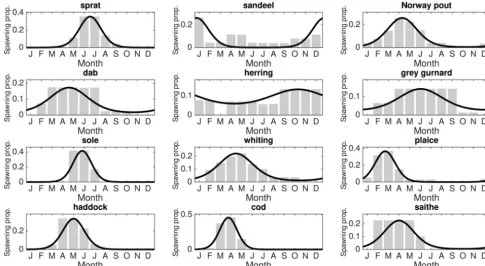
Spawning patterns are another important source of temporal variation in marine systems. It is well established that some fish species such as cod, sole, and sprat (see, e.g.,Mertz and Myers 1994;Johnson 2000;Armstrong et al. 2001) spawn only at certain times in the year to take advantage of the extra food abundance from annual phytoplankton plankton blooms, if Cushing’s “match–mismatch” hypothesis is to be believed (Cushing 1975; Beaugrand et al. 2003). However, different species living under the same conditions have vastly different spawning patterns (see Fig. 1), and it is important to include in any reproductive model the range of strategies adopted by different species.

Dynamic size spectrum models are increasingly being used to understand structure and dynamics of marine systems, including the effects of fishing and climate change (Blanchard et al. 2012; Woodworth-Jefcoats et al. 2013) and inclusion of multispecies dy-namics to address questions related to fisheries (Blanchard et al. 2014; Spence et al. 2016). However, so far, these models have simplified reproductive processes and focused on interannual changes in plankton levels.

Modelling reproduction in a size spectrum model has been ac-complished previously in a nonseasonal setting (e.g.,Maury et al. 2007a;Hartvig et al. 2011;Law et al. 2012); in short, models gener-ally used a fraction of the assimilated body mass from predation to produce eggs of a fixed mass, following the dynamic energy budget (DEB) theory ofKooijman (1986,2009). This resulted in an influx of biomass at a fixed offspring mass in the spectrum, fol-lowing the observation that regardless of fish species, egg size is fairly constant among many pelagic fish species (Ware 1975;Cury and Pauly 2000). Physiologically structured population models (PSPMs) often include pulsed reproduction in which preallocated mass is transformed into a batch of new cohorts at the beginning of each season (see, e.g.,Persson et al. 1998;De Roos and Persson 2001). More recently, PSPMs have allowed reproduction to occur over longer discrete time intervals (Huss et al. 2012;van Leeuwen et al. 2013). More complex individual-based size-structured models have incorporated seasonal reproduction dynamics but focused either on a specific region geographically (Marzloff et al. 2009) or on consumer–resource dynamics without the effects of predation on consumers (De Roos et al. 2009;Sun and de Roos 2015).

A recent paper bySainmont et al. (2014)used an ordinary differ-ential equation (ODE) model approach to investigate alternative strategies for seasonal reproduction (capital versus income breed-ing) in environments with varying feeding seasons and maturity masses. In short, income breeding allocates incoming mass di-rectly to reproduction, whereas capital breeding stores reserves that may be used for spawning at a later time, independent of food availability. That paper found capital breeding to be the optimum strategy in higher latitude environments where food availability was more variable (with a sharp spike in springtime and lower levels outside this period), with income breeding being advanta-geous for longer feeding seasons. For more details about capital and income breeding, seeJönsson (1997),Jager et al. (2008), and Ejsmond et al. (2015).

Clearly, a comprehensive simulation of the impacts of season-ality should include capital breeding, as this strategy can be both

optimal theoretically (Sainmont et al. 2014;Ejsmond et al. 2015) and, more importantly, common empirically in seasonal environ-ments (e.g.,Lambert and Dutil 2000). However, the purpose of this study is to conduct an initial exploration of the consequences, for the consumer size spectrum, of seasonality in both resource avail-ability and consumer spawning times. Given that this is an introductory analysis of the qualitative effects of these seasonal patterns on the dynamics and behaviour of consumer spectra, the focus will be on income breeding, perhaps the simplest repre-sentation of how energy is allocated between reproduction and growth in the face of seasonal variation in resource availability, as modelled previously (Law et al. 2012;Blanchard et al. 2014;Scott et al. 2015). We expect that the results of this analysis will guide future work on including and evaluating the impact of capital breeding behaviour on seasonal patterning of the consumer spectrum.

This study builds upon previous work on the timing of larval hatching in which a fixed temporal “background” spectrum was set up and then cohorts born at different times were followed to calculate the best time of year to be born in terms of fast growth and low mortality, without modelling the dynamical feedbacks to the size spectrum (Pope et al. 1994). That paper found that it was best to be born at or before the peak in plankton abundance to avoid increased predation mortality from the fixed wave reaching the size range of predators of newborns and to stay ahead of this wave for the rest of the year.

Here we introduce seasonality to a previously published multi-species size spectrum model (Blanchard et al. 2014;Scott et al. 2015) to investigate the properties of seasonal size spectra. To do this, we introduce a dynamic, time-varying phytoplankton spec-trum over the year, as well as seasonal spawning, for 12 North Sea fish species (sprat (Sprattus sprattus), sandeel (Ammodytes marinus), Norway pout (Trisopterus esmarkii), dab (Limanda limanda), herring (Clupea harengus), grey gurnard (Eutrigla gurnardus), sole (Solea solea), whiting (Merlangius merlangus), plaice (Pleuronectes platessa), had-dock (Melanogrammus aeglefinus), cod (Gadus morhua) and saithe (Pollachius virens)) fitted to empirical spawning data. The interplay of seasonal effects with the basic life processes of growth, predation, reproduction, and death leads to high variability in the fish species spectra compared with nonseasonal systems. As an example of the uses of this dynamic model, we investigate several properties of the size spectrum under seasonal and nonseasonal conditions. These included the long-term behaviour of the slope of the size spectrum under different fishing regimes, as well as changes in fishing yields.

Methods

Setting up the size spectrum model

To model seasonal reproduction of pelagic predators (typically fish) and plankton blooms, a modified version of the previously published “mizer” package in R is used (Scott et al. 2015), which uses the work ofBlanchard et al. (2014)as its basis. The model of that paper is a representation of the North Sea community, with parameters calibrated to observed catch and effort data for the North Sea over the period 1985–1995. Hence, this study is, in part, an extension of the work presented inBlanchard et al. (2014)and will necessarily be conditioned by the structure and assumptions of that work, specifically:

1. model responses to both the addition of seasonal affects and changes in fishing pressure will be conditioned by how this set of North Sea species was harvested over the calibration period 1985–1995;

2. the calibration procedure used in the 2014 study will have a significant effect on the role that changes in egg production can have in this new study; more detail on this will be pro-vided in the description of how reproduction is represented in this model.

Can. J. Fish. Aquat. Sci. Downloaded from www.nrcresearchpress.com by Canadian Science Publishing on 05/12/16

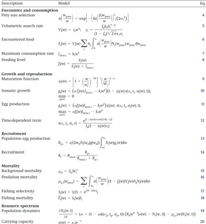
The model presented here consists of two parts: a resource spec-trum and a multispecies consumer specspec-trum, both of which are dynamic and time-dependent. Here, “consumer” refers to organ-isms within any of the fish species spectra, and the aggregation of all species spectra is labelled the “community” spectrum. The “resource” spectrum comprises both the phytoplankton and zoo-plankton communities. We summarise the model used in the following subsections; for further information on the equations and parameters used, seeTable 1; default parameter values are used for all simulations, as in the mizer vignette (Scott et al. 2015, p. 67). Values for parameters related to seasonal spawning and plankton blooms are given inTable 2. Supplementary material S12 describes how to add seasonality to the mizer model, along with a link to the R code used; what follows here is an in-depth look at the model structure.

Consumer spectrum

The model uses the McKendrick – von Foerster equation as its backbone for growth through the spectrum (Andersen and Beyer 2006;Blanchard et al. 2009;Law et al. 2009;Datta et al. 2010). Organisms feed upon smaller organisms in both the resource and consumer spectra according to a Gaussian feeding preference function (Table 1,eq. 4), commonly used in modelling predation in marine systems (Benoît and Rochet 2004;Andersen et al. 2009; Law et al. 2012). Organisms die either from being eaten by larger organisms or from natural causes (this encompasses starvation and natural mortality; seeTable 1). Starvation has often been cited as a source of high mortality for fish (although results are not entirely conclusive; seeAnderson (1988)) and is included as a func-tion that becomes more severe as the growth rate of consumers drops; it decreases exponentially with body size, as larger body

size makes starvation less likely (Duarte and Alcaraz 1989;Leggett and Deblois 1994).

Because the mass of eggs spawned from marine teleost fish lies in a narrow range around 1 mg (Ware 1975;Cury and Pauly 2000), recruitment to a single fixed egg mass (of 1 mg) in the spectrum is used. Reproduction can be either constant or over a limited period of time across the year. The reproductive rate is dependent on the predation rate, in keeping with the dynamic energy budget meth-ods (Kooijman 2009) commonly used in size spectrum models to allocate incoming mass to somatic and reproductive mass (e.g., Maury et al. 2007a;Blanchard et al. 2011). Thus we consider mature individuals to be income rather than capital breeders, the latter having spawning that is relatively independent of current prey availability but strongly dependent upon lagged average availabil-ity (Sainmont et al. 2014). The physiology of egg production is not explicitly modelled, and simple size-based fecundity is assumed.

The incorporation of reproduction into the model follows the mizer model (Scott et al. 2015,eq. 3.10), although here we also include a time-dependent term to allow for seasonal spawning. This time-dependent term generates temporal change for both seasonal spawning and plankton pulses and is adapted from pre-vious work (Pope et al. 1994;Datta 2011). It has the form

(1) s(␯_i,t_i,␺_i,t)⫽e

(1⫺␺i)␯icos(2␲(t⫺ti))

I₀((1⫺␺_i)␯_i)

and is a dimensionless term dependent on time (t), wheret_iis the time of the pulse peak, and␯idescribes the severity of the peak

(i.e., how short and sharp spawning or the bloom is over the year). For reproduction, the two parameterstiand␯iare fitted

2_{Supplementary material is available with the article through the journal Web site athttp://nrcresearchpress.com/doi/suppl/10.1139/cjfas-2015-0468.}

Fig. 1. Fitting von Mises distributions to the 12 fish species simulated in the model. The fit consists of two parameters for each speciesi:ti, the

time of maximum spawning;␯i, the severity of the spawning peak. The species are, in increasing asymptotic size from left to right and top to

bottom: sprat, sandeel, Norway pout, dab, herring, grey gurnard, sole, whiting, plaice, haddock, cod, and saithe. Data aggregated fromBowers (1954),Quéro (1984),Alheit (1988),Knijn et al. (1993),Albert (1994),Brander (1994), andHunter et al. (2003).

Can. J. Fish. Aquat. Sci. Downloaded from www.nrcresearchpress.com by Canadian Science Publishing on 05/12/16

to empirical data on spawning patterns of the 12 fish species modelled (Fig. 1), while for resource blooms, the parameters are estimated from observed data (see Table 2). I0 is the modified Bessel function of order 0 and is a normalising factor that fixes the total mass allocated by an individual to spawning over a year for all␯i. In other words, as␯iincreases, the duration of spawning

becomes shorter, giving a narrower Gaussian-shaped peak (the numerator ofeq. 1). However, a higher␯icauses the denominator

I0to decrease, increasing the height of the peak to give the same area under the curve (i.e., an equal number of eggs). Thus, altering spawning duration for a species produces an equivalent amount of offspring (for equal feeding rates). In Supplementary material

S2,2_s(␯

i,ti,␺i,t) is plotted for a range of values of␯ito illustrate

this.

We introduce the following terminology to describe aspects of the reproductive process in the model:

• individual reproductive investment: the proportion of incom-ing mass that an individual uses for egg production (Table 1, eq. 11). This depends upon an individual’s species, its mass (w), and time (t) and is limited by incoming biomass at each time step.

• population reproductive investment: the aggregated popula-tion producpopula-tion of eggs for a species (Table 1,eq. 13). This is

Table 1.Size spectrum model equations.

Description Model Eq. no.

Encounter and consumption

Prey size selection

␾

冉

w

冊

冋

冉

冉

␤iwprey

w

冊冊

2

/

共

兲

册

Volumetric search rate

V_i(w)⫽␥_iwq; ␥_i⫽ f0hi␤i

n⫺q

(1⫺f₀)兹2␲␬_r␴_i

5

Encountered food

E_i(w)⫽V_i(w)

兺

j

␪ij

冕

0

∞

␾

冉

w

冊

6

Maximum consumption rate I_max.i⫽h_iwn ₇

Feeding level

f_i(w)⫽ Ei(w)

E_i(w)⫹I_max.i

8

Growth and reproduction

Maturation function _␺

i(w)⫽

冋

冉

w w_i∗

冊

⫺10

册

冉

冊

1⫺n ₉

Somatic growth g_i(w)⫽

共

兲

gi(w) ⫽

0

10

Egg production _g

r(w)⫽

共

p

兲

i(w) ·s(␯i,ti,␺i(w),t),

max

gr(w) ⫽␣

f_i(w)I_max.i⫺k_iwp

11

Time-dependent term

s(␯i,ti,␺i,t)⫽

e(1⫺␺i(w))␯icos(2␲(t⫺ti))

I₀(1_⫺␺_i(w)␯_i)

12

Recruitment

Population egg production

R_p.i⫽⑀/(2w₀N_i(w₀)g(w₀))

冕

wi∗

wi

N_i(w)g_r(w)dw

13

Recruitment

R_i⫽R_max.i Rp.i R_max.i⫹R_p.i

14

Mortality

Background mortality _␮0⫽Z₀W_iz ₁₅

Predation mortality

␮p.i(wprey)⫽

兺

j

冕

∞

␾

冉

w

冊

16

Fishing selectivity _S

i(w)⫽1/(1⫹e(S1⫺S2w)) 17

Fishing mortality F¯i(w)⫽Si(w)Fi 18

Resource spectrum

Population dynamics ⭸N_r(w,t)

⭸t ⫽(␻ ⫹(1⫺␻)s(␯p,tp,␺p,t))·

共

n⫺1_[␬(w)⫺N

r(w,t)]⫺␮p.r(w)Nr(w,t)

兲

19

Carrying capacity _␬(w)⫽␬

rw⫺␭ 20

Note:Species-specific parameters are defined as follows for speciesi, in order of appearance:␤i, preferred predator–prey mass ratio;

␴i, width of prey size preference;␥i(g–q·year–1), volumetric search rate;h(g1−n·year–1), maximum food intake rate;␪ij, interaction with

speciesj;wi∗(g), maturation weight;Wi(g), asymptotic weight;ki(g1−n·year–1), standard metabolism;Ni, population density;Rmax.i

(density·year–1_{), estimated maximum recruitment parameters;F}

i, fishing selectivity parameter. Constants are defined as follows, in

order of appearance:f0, critical feeding level;q, exponent of search volume;n, exponent of maximum consumption;␬r, carrying

capacity of resource spectrum;␣, assimilation efficiency;p, exponent of standard metabolism;⑀, reproductive efficiency;w0, egg

weight;Z0, pre-factor for background mortality;z, exponent of background mortality;S1 andS2, fishing selectivity weights;R0,

productivity of resource spectrum;␭, exponent of resource spectrum. For values of all parameters (except those related to seasonality), see (Blanchard et al. 2014, tables S2 and S5). For detailed information about the life processes modelled, see (Scott et al. 2015, section 3).

Can. J. Fish. Aquat. Sci. Downloaded from www.nrcresearchpress.com by Canadian Science Publishing on 05/12/16

summed over all mature individuals in the species (the integral term ofeq. 13inTable 1) and takes into account production efficiency and the sex of individuals (Scott et al. 2015, section 3.5). • recruitment: the total number of eggs feeding into the “new-born” mass bin of a species at timet, which takes into account the maximum level of recruitment for each species (Table 1,eq. 14).

Given the parameterisation inBlanchard et al. (2014), we ex-pected that recruitment for all species would remain at or close to their maximum (Rmax.iineq. 14ofTable 1) for all times and

sce-narios, and this expectation was borne out in practice during initial runs of the model. As a consequence, behavioural patterns observed in model output of this study are interpreted in terms of the shifts in growth and mortality rates that are produced by introducing seasonality.

The mass parameter␺is the allocation of incoming mass to reproduction rather than somatic growth, which incorporates both the maturation mass and asymptotic mass of a species (Table 1,eq. 9). Without the (1 –␺) terms,eq. 1is the von Mises function used byPope et al. (1994), and for plankton blooms, we set ␺p= 0 to give this form. The (1 –␺) terms are included for spawning to limit the growth of organisms close to their asymp-totic mass by forcing them to spawn less seasonally as their mass increases. This assumption is not realistic, but within this model-ling framework, it is a necessary addition for growth behaviour of the species to match the fitted growth curves ofBlanchard et al. (2014). Those curves implicitly assumed constant reproduction as a fraction of incoming mass and to disentangle the process would require an entirely novel parameterisation for the growth of all species and was beyond the scope of this work. The assumption is discussed more in the Discussion.

Using empirical data on the monthly spawning rates for the 12 fish species simulated, von Mises distributions (Pope et al. 1994) are fitted to each species to give the shape of the reproduction curves (Fig. 1).

In Supplementary material S3,2 _{a methodological derivation} for the reproduction function used in mizer (Scott et al. 2015) is shown, using similar methods to the derivation of the determin-istic jump-growth model (Datta et al. 2010); in short, it is assumed that the amount of mass lost in each spawning event is quite small, leading to a first-order approximation that can potentially be incorporated into any McKendrick – von Foerster equation to simulate both capital and income breeding processes.

Fishing is incorporated as inBlanchard et al. (2014); relevant equations are shown inTable 1, eqs. 17 and 18. In summary, fishing mortality is size- and species-specific, which can remain constant throughout the simulation or can vary at specified times. A stan-dard fixed logistic selectivity function is used to describe the ability of the fishery to catch each species. Parameters are selected so that baseline fishing efforts give realistic distributions for the

species spectra, using stock assessment data from the period 1985–1995 (www.ices.dk). Some parameters are non-species-specific and are assumed to be the same for all species. For a full list of parameters and values, see tables S2 and S3 ofBlanchard et al. (2014).

Resource spectrum

For simplicity, the processes driving the dynamics of phyto-plankton and the acquisition of energy from nutrients and light are not explicitly modelled here (see Moloney and Field 1991; Fuchs and Franks 2010). Instead, it is assumed that organisms in the resource spectrum can be preyed upon by organisms in the consumer spectrum but replace themselves using a semi-chemostat function for replenishment to a carrying capacity. Models have tested the response of the size spectrum to bottom-up perturbations before by increasing the height of the phytoplankton size classes uniformly for a short period of time (Maury et al. 2007b;Blanchard et al. 2011). Here a similar approach is taken.

Following the approach ofPope et al. (1994), the seasonal size– time resource spectrum is characterised by the von Mises time distribution (eq. 1), as well as predation by the consumer trum, and the equation for the dynamics of the resource spec-trum is given by

(2) ⭸NR(w,t)

⭸t ⫽(␻ ⫹(1⫺␻)s(␯p,tp,␺p,t))·N

The left-hand side denotes the change over time in the resource spectrumNR, which is a function of mass (w) and time (t).Nis the shorthand introduced for the dynamics of the resource spectrum of eq. 3.15 ofScott et al. (2015). The preceding term differentiates our model from the original;␻sets what proportion of the spec-trum is present independent of the bloom, ands(␯p,tp,␺p,t) sets the shape of the bloom (there is no mass-dependent behaviour for the bloom, so␺p= 0 for all size classes in the resource spectrum). Resource abundance thus remains relatively constant for most of the year but then, dependent on the value of␯p, may “bloom” for a short period, that is, the entire resource spectrum increases in abundance, while keeping the same gradient, before relaxing back to its original level.

Parameters are chosen to reflect the likely timing and abun-dance of blooms in real systems (Gasol et al. 1991;Huete-Ortega et al. 2010). The increased abundance affects the feeding rate, and thus growth, of consumers able to take advantage of the increase in biomass in the system. The full form ofeq. 2is given inTable 1, eq. 19.

The combination of bottom-up and top-down feedbacks is what the simulations focus on and is a natural progression from the

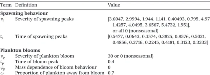
Table 2.Parameter values used for seasonal processes in the model.

Term Definition Value

Spawning behaviour

␯i Severity of spawning peaks [3.6047, 2.9994, 1.944, 1.141, 0.40493, 0.795, 4.973,

1.4257, 4.0495, 3.6567, 5.4732, 1.951], or all 0 (nonseasonal)

ti Time of spawning peaks [0.5477, 0.0643, 0.3574, 0.3825, 0.8576, 0.5021,

0.4856, 0.3716, 0.2245, 0.4181, 0.3123, 0.3333]

Plankton blooms

␯p Severity of plankton bloom 30 or 0 (nonseasonal)

tp Time of bloom peak 0.4

␺p Mass dependence of bloom behaviour 0

␻ Proportion of plankton away from bloom 0.7

Note:The shape of plankton blooms is taken from empirical data sources (Gasol et al. 1992;Huete-Ortega et al.

2010). Parameters related to spawning are fitted to species-specific spawning data (Fig. 1); numbers refer to species in order, from left to right and then top to bottom.

Can. J. Fish. Aquat. Sci. Downloaded from www.nrcresearchpress.com by Canadian Science Publishing on 05/12/16

previous work byPope et al. (1994)in which the entire size spec-trum was specified by a von Mises distribution; here the interplay between differently timed seasonal processes is what drives the dynamics to produce qualitatively different community spectra. Differences in the two analyses are further reviewed in the Discussion.

Numerical simulations

To numerically solve the dynamics of the model, the system of resource and fish species spectra is initialised using default values fromScott et al. (2015). This is taken as the initial distribution for all of the simulations. The resource and fish species spectra through time are then calculated, both with and without seasonal plankton blooms and seasonal spawning (henceforth referred to as seasonal and nonseasonal systems, respectively).

The growth trajectory of an individual is tested using the method of characteristics (see Kot (2001), p. 393 onwards). The body mass of a newborn through time is calculated by solving

(3) dw

dt ⫽gi(w(t))

wheregi(w(t)) is taken fromeq. 10ofTable 1. The method of

char-acteristics is employed to calculate the growth trajectories (eq. 3) of offspring of the different species over the course of a lifetime, as in previous work (Law et al. 2009;Rochet and Benoît 2012). In short, the starting mass of the individual is set at the mass of a newborn (1 mg). Then, at each time step, the growth rate of the individual is set at the mass bin that the individual occupied, and the new mass is calculated. By tracking this mass through time, we calculate how quickly organisms grow in nonseasonal and seasonal spectra.

The effect of seasonal reproduction on the dynamics of the con-sumer spectrum is investigated to simulate the spawning behaviour of 12 North Sea pelagic fish species (Fig. 1). A fixed resource and community spectrum, which included waves of abundance from phytoplankton blooms, was previously studied without dynamical links between growth, mortality, and reproduction dynamics (Pope et al. 1994). We extend this model framework by making both spec-tra fully dynamic and including species-specific seasonal spawning. The growth of individuals within both nonseasonal and seasonal

systems are compared; this consists of growth within the spectrum, behaviour of the community spectrum slope (calculated by fitting a linear model to the plot of number density against mass, between 1 g and 10 kg, using a natural logarithm), and fishing yields over time.

All simulations are carried out using R (R Core Team 2015). For each simulation, the spectrum is allowed to run for 500 years with weekly time steps so that a steady state for the nonseasonal sys-tem is reached and the seasonal syssys-tem has extremely similar patterns between years before analyses are carried out.

Results

The size spectrum with nonseasonal and seasonal processes

The size spectra at the end of 500 years under both nonseasonal and seasonal conditions are shown inFig. 2. The community spec-trum (averaged over a year) is similar for the nonseasonal and seasonal systems (Fig. 2a). In either case, the community spectrum rapidly settles down to a ridged uneven shape above 10 g, caused by the range of asymptotic sizes reached by the 12 species. This shape was also noted previously byBlanchard et al. (2014)when running the system to steady state. There exists a discontinuity in the gradient of the slope at the boundary between the resource and consumer spectra where offspring are born, consistent with similar previous studies (Blanchard et al. 2011). The shapes of the community spectra can be better understood by examining the individual species spectra (Fig. 2b), where the species grow to different asymptotic masses; this leads to the irregular shape of the community spectrum. Both the nonseasonal and seasonal spe-cies spectra are visually similar, and hence, only the seasonal system is plotted here.

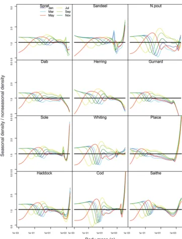
Although the annual averages of both community spectra ap-pear similar, within a year, there is much variation in the species spectra in the seasonal system. This is shown in Fig. 3, where densities at size are plotted relative to the nonseasonal steady state spectrum. At the low end of the species spectra, there are high variations in abundance due to the uneven spawning pat-terns of the species. A wave-like pattern propagates through the species spectrum as extra biomass from the resource bloom al-lows for faster growth of the smallest individuals in the spectrum, leading to a drop in number density in the smallest size classes and increased number density further along the size spectrum.

Fig. 2. The size spectrum after 500 years, with nonseasonal and seasonal processes in place. (a) Comparing the community spectra for nonseasonal (dashed black line) and seasonal (solid grey line) systems. Also included for reference is the nonseasonal resource spectrum (dotted black line at left side of the spectrum). (b) The seasonal size spectrum after 500 years; community spectrum given by solid black line, individual species spectra shown by dashed grey lines. Asymptotic size of each species marked by black squares.

Can. J. Fish. Aquat. Sci. Downloaded from www.nrcresearchpress.com by Canadian Science Publishing on 05/12/16

These waves are damped at larger masses as organisms undergo growth, death, and reproduction through the spectrum, leading to a smoothing effect due to lowered biomass. At the right end of the spectrum, the ratio for some species becomes very large or small due to tiny abundances at high masses in both spectra, so that small variations have large impacts. However, there are two groups of species with different patterns: one with lower abun-dance density at largest sizes (sprat, dab, herring, gurnard) and the other with higher densities at large sizes (e.g., sandeel, sole, plaice, haddock, cod, saithe) relative to the nonseasonal model. This is an emergent result of the model due to faster growth and larger size at age reached for the latter group of species (Fig. 4), whereas for the former group, growth was either very similar or lower.

Growth within seasonal systems

In the nonseasonal system, growth curves over lifetimes were previously cross-validated with empirically fitted von Bertalanffy growth curves for each species (Blanchard et al. 2014). Comparison of growth in a seasonal versus nonseasonal system also reveals increasing temporal variation as fish become mature (Fig. 4). Somatic growth is slower during the spawning period than the rest of the year. Species with narrower periods of spawning (see Fig. 1) have less smooth growth curves; for example, compare the trajectories of cod and sole, which have highly seasonal spawning, with those of grey gurnard and Norway pout, which spawn more evenly throughout. The overall growth over several years is simi-lar to the nonseasonal system, with the same asymptotic masses being reached; this is due to the setup of the reproduction function

Fig. 3. The bimonthly size spectra over a year for the 12 fish species in a seasonal system, relative to their (nonseasonal) steady state abundances (horizontal black lines), to elucidate the differences between the systems. Months are plotted in different colours to allow comparison between times and species.

Can. J. Fish. Aquat. Sci. Downloaded from www.nrcresearchpress.com by Canadian Science Publishing on 05/12/16

(eq. 1), which makes spawning less seasonal as the asymptotic mass is reached.

The growth rate of a mature individual is shown inFig. 5 com-pared with a nonseasonal spawner. Initially, reproductive effort is low, so the majority of biomass is used for somatic growth; hence, the gradient of the growth is steeper than for a nonseasonal spawner whose growth rate is relatively constant over the whole year. As the reproductive period begins, overall growth decreases and drops to zero around timet= 0.35. Negative growth is not permitted in the model (as we are using income breeding), and when spawning is near its peak, growth remains at zero, with all incoming mass being allocated to egg production. Aroundt= 0.75, growth increases again, mirroring the von Mises spawning distribution closely. If a capital breeding function were used (i.e., making the somatic growth rate (Table 1,eq. 10) and egg produc-tion (Table 1,eq. 11) independent of each other), there would be the possibility for individuals to lose mass over the reproductive period, which would depend upon the rates of growth and spawn-ing. In laboratory studies, body mass has been observed to de-crease if the mass lost in spawning is not compensated by the biomass assimilated through predation (Wootton 1977;Lambert and Dutil 2000), and the condition factor (related to mass at length) of fish has been shown to drop after spawning (Le Cren 1951;Pedersen and Jobling 1989).

Size spectrum properties in seasonal and fished systems

The effect of seasonality on the community spectrum slope is shown inFig. 6a. The initial slope is approximately –1.65 (this is maintained under baseline fishing effort). After fishing intensity is doubled, the slope for both seasonal and nonseasonal systems

Fig. 4. The growth curves (calculated using the method of characteristics (eq. 3)) for offspring of different species hatching into spectra in both nonseasonal (dashed grey lines) and seasonal (solid black lines) systems, over 15 years.

Fig. 5. The growth trajectory for a mature sole individual in a seasonal environment (solid black line) compared with a similar-sized individual in a nonseasonal environment (dashed grey line). Shown for reference is the spawning function for sole (dotted black curve), taken fromFig. 1.

Can. J. Fish. Aquat. Sci. Downloaded from www.nrcresearchpress.com by Canadian Science Publishing on 05/12/16

decreases to around –1.9. The nonseasonal system settles to a steady state rapidly, while the seasonal system oscillates at an average slightly above this value, with a cycle of 1 year, owing to seasonal processes occurring at the annual time scale. Halving fishing effort leads to an increase in the slope of the spectrum due to a lack of fishing mortality for fish on the right-hand side of the spectrum, reaching around –1.5 for both systems; the slope in the seasonal system oscillates around an average value slightly below that observed in the nonseasonal system. These qualitative re-sponses of slope to changes in fishing effort should be regarded as particular to our North Sea model, as they are conditioned by how our model represents the species-specific interplay be-tween fishing effects and the growth pulse driven by the re-source bloom.

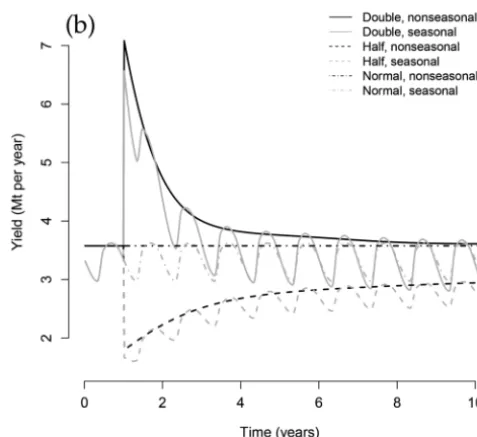
At baseline fishing effort, yields for seasonal systems tend to be lower than nonseasonal systems and peak around the nonsea-sonal yield (Fig. 6b). This is due to the long-term distribution of the seasonal community generally having a higher abundance of smaller individuals but fewer large individuals, resulting from the effect of seasonal processes on growth of individuals to the larger size classes (Fig. 7).

After fishing efforts are doubled, yields initially spike to around twice the original quantity; however, in the following years, yields quickly drop as the increased mortality from fishing forces the community spectrum into a steeper shape, with lower abundance of larger fish (Fig. 6b). Yields settle at about their original quantity within 10 years, despite fishing pressure remaining twice as high. The opposite behaviour is seen when fishing intensity is halved; an initial drop in yields is followed by a gradual increase (due to lower mortality rates for mature fish leading to a more abundant community), settling at a value of 2.95 Mt·year–1_{, slightly lower} than at baseline effort (3.58 Mt·year–1_{). Seasonal yields follow the} same pattern as nonseasonal systems, although they oscillate around a lower mean value; only at oscillation peaks are yields roughly equivalent to the nonseasonal spectrum, and at the troughs, they are approximately 80% of the nonseasonal yield. Increasing fishing effort in seasonal systems makes the variability

Fig. 6. The effect of altering fishing intensity after a year on (a) the community spectrum slope and (b) total fishing yields. Nonseasonal spectra shown in black, seasonal in grey; solid lines indicate doubling fishing intensity, dashed lines indicate halving, and dotted–dashed lines indicate maintaining baseline fishing effort. The baseline fishing effort consists of estimates used to calibrate the model across the 1985– 1995 time period, and cross-validation was shown to give realistic time-averaged species size distributions and growth in nonseasonal species spectra (Blanchard et al. 2014).

Fig. 7. The abundance of individuals for nonseasonal and seasonal systems over 10 years with baseline fishing effort, once systems have reached regular interannual patterns. Shown are total number densities for organisms (a) less than 40 g and (b) greater than or equal to 40 g. Black solid lines indicate nonseasonal systems, and grey dashed lines indicate seasonal systems.

Can. J. Fish. Aquat. Sci. Downloaded from www.nrcresearchpress.com by Canadian Science Publishing on 05/12/16

in yields greater (comparing the difference in peaks and troughs between double and half fishing effort inFig. 6b).

However, integrated across the entire year, whichever fishing strategy is picked, the ratio of the seasonal to nonseasonal yields is close (approximately 93%). This is ultimately due to the fact that, in the region of parameter space that the model occupies, juvenile production is fairly constant between years (due to recruitment being more or less equal for nonseasonal and seasonal systems), but adult population densities are more often lower for seasonal than for nonseasonal spectra, resulting in lower fishing yields.

Discussion

Seasonal processes induce time-varying behaviour in the size spectra for individual species, with markedly different intra-annual growth for mature individuals. Although the aggregated community spectra remain visually similar for both seasonal and nonseasonal systems, analysis of these communities reveals key differences. The spectrum slope is more varied in seasonal systems, while fishing yields are up to 20% lower than under nonseasonal conditions during the year. In the seasonal system, increased fishing effort amplifies the peaks and troughs in the species size spectra, and hence, the yields become much more variable through time (Fig. 6b). In aquatic systems, increases in fishing effort have led to a shift towards faster growth rates, which have previously been shown to cause increased temporal variability in production and fisheries yields (Blanchard et al. 2012). Arguments about balanced harvesting have also been made on the basis that fisheries size-selectivity affects the stability of size spectra and yields (Law et al. 2012), but this has yet to be investigated in the context of seasonal dynamics. Seasonal pro-cesses may thus have important implications for conclusions about fisheries management.

Compared with the value of –1 often seen in aquatic systems (e.g.,Boudreau and Dickie 1992;San Martin et al. 2006;Zhou et al. 2009), the slopes observed here are steeper; however, heavily ex-ploited systems have been shown to produce steeper slopes in the past due to fishing-induced truncation of the spectrum (Rice and Gislason 1996;Blanchard et al. 2005). Seasonality led to a higher variability in the community spectrum slope than in its absence. Spawning strategies ranged from matching closely with the timing and duration of the plankton bloom (e.g., sole and Norway pout inFig. 1) to those spawning far away from the bloom (e.g., sandeel). However, the balance of matches and mismatches of spawning and blooms does not account for the variation in slopes. Rather, within-year variation was due to the interplay between increased growth of smaller individuals caused by the annual plankton bloom, leading to a qualitatively different community spectrum with varied intra-annual dynamics but fairly similar interannual behaviour. We were aware that the region of param-eter space that the model occupied had high levels of recruitment, withRiclose toRmax.ifor all species and times (Table 1,eq. 14), and

this limited the effect that seasonal reproduction had on the spe-cies spectra (as changes in recruitment were extremely minor over the course of a year). In reality, density-dependent recruit-ment is an important factor in constructing size spectrum models and requires a more in-depth approach in the future (Andersen et al. 2016, pp. 18–19).

The resource bloom provided the majority of the changes in slope in this study. It was observed that, regardless of what upper and lower mass limits were chosen when calculating the slope, the qualitative behaviour when altering fishing effort was the same (as inFig. 6a). Mass limits between1 g and 10 kg were chosen here as representative of the community. Altering these could affect the magnitude of shift in average seasonal slope compared with the nonseasonal slope, but the overall trend of steeper slopes with increased fishing persisted regardless.

Adding seasonality induced waves of biomass that moved up the species spectrum, as growth rates and offspring populations rose and fell throughout the year (Fig. 3). There was a peak in biomass in offspring at the appropriate spawning peak fromFig. 1; however, this was not as pronounced as the dip in biomass during the plankton bloom due to the increased growth rate of newborns caused by a more abundant food supply in this period. Waves of abundance have been observed in previous models (Law et al. 2009;Datta et al. 2010) when parameter values were chosen that destabilised the steady state distribution. Adding a plankton bloom has a similar effect, as organisms whose feeding range lies within the plankton spectrum are subject to higher growth rates (Benoît and Rochet 2004;Maury et al. 2007a). Here it was observed that seasonal forcing via the reproductive process also pushes the system away from the steady state. With both plankton blooms and time-dependent reproduction occurring simultaneously, depar-tures from the well-established power-law distribution (Sheldon et al. 1972) are expected.

As expected, the general trend was for slopes to have a steeper gradient as fishing effort increased, due to higher mortality on organisms with higher mass (Fig. 6a). Interestingly, doubling fish-ing effort initially gave higher yields but these quickly declined to a level similar to that provided by the baseline effort; halving effort had the opposite effect of an initial decline before increas-ing, with an asymptote of a slightly reduced yield compared with baseline effort (Fig. 6b). Upon investigation, the cause was not shifts in the biomass of newborns, which was not significantly perturbed. Rather, the total biomass of the larger fish (the seg-ment of the spectrum targeted by fishing) moved to different levels under the new fishing regimes, with doubled effort leading to a decrease in the biomass of larger fish and halved effort lead-ing to an increase. We stress that many of the model parameters of mizer are derived using the baseline fishing effort (time-averaged estimates over 1985–1995), so we do not draw heavy conclusions from this result except that doubling these values in the long-term produced yields more consistent with the flat part of a yield curve (they did not increase much) but carried a greater impact on the community size spectrum.

In all cases (baseline, doubled, and halved efforts), seasonality led to yields fluctuating near the nonseasonal value at their peak, but with a lower average and troughs around 80% of the nonsea-sonal yield. It is perhaps not surprising that the nonseanonsea-sonal sys-tem set the upper limit for yields, as for both syssys-tems recruitment was fixed byeq. 14ofTable 1; with species-specific fishing pressure and asymptotic sizes, these factors resulted in a similar upper limit for the number of mature individuals in the community for seasonal and nonseasonal systems. Future work on the parameter sensitivity and uncertainty (Spence et al. 2016) is needed to eluci-date the trade-offs in yield that result under different environ-mental conditions and management strategies. It is well known that fish stocks greatly fluctuate intra-annually (Horwood et al. 2000), and the simulations here show that assuming a nonseasonal system means higher yield predictions than when incorporating sea-sonality. For more accurate fisheries management, including time-dependent processes such as spawning could help improve the predictive powers of models to judge expected catch sizes through-out the year. This model could be used in conjunction with other operating models as part of management strategy evaluation to as-sess consequence of both short-term changes in seasonality and lon-ger term environmental variability and change.

Size-based models have commonly divided incoming biomass from the predation process into somatic growth and egg produc-tion (De Roos and Persson 2002;Maury et al. 2007a;Kooijman 2009;Blanchard et al. 2011;Hartvig et al. 2011). We followed the same method here (Scott et al. 2015, section 3.4), but importantly allowing spawning to take place over limited times of each year. This is a natural step forwards from the early theoretical analysis ofPope et al. (1994), who used a static spectrum to investigate the

Can. J. Fish. Aquat. Sci. Downloaded from www.nrcresearchpress.com by Canadian Science Publishing on 05/12/16

growth and survival trajectories of cohorts born at different times of year. While we have not tested the success of different spawn-ing techniques here, we have laid important groundwork in pro-viding a more realistic framework in which the importance of spawning strategy in maximising cohort growth and maturation can be investigated. Having said that, there are several important caveats that could guide further developments.

An assumption introduced for convenience was to make spawn-ing less seasonal as the asymptotic mass of an individual was approached. This limited the growth of species to empirically reasonable values; however, in reality, seasonally spawning spe-cies retain seasonality, even at the largest size classes. This ex-plains the similarity between the steady state species size spectra in the seasonal and the nonseasonal scenarios (Fig. 2). Older indi-viduals make a relatively large contribution to overall population fecundity; thus, the effect of spawning seasonality (as currently depicted in the paper) on species dynamics may well be underem-phasized. Hence, an important part of the follow-up work would be to incorporate more realistic growth functions for seasonally spawning species such that both seasonal reproduction and a re-alistic upper body size for each species can be achieved.

Quantification of the size and timing of the plankton bloom was illustrative for the model. These factors are not constant globally and are affected by, for example, latitude, temperature, and hy-drodynamics, as well as natural interannual variability. Here a single set of parameters was selected for the model; the peak of the bloom was around six times the abundance of outside the bloom period, and the bloom lasted around 7 weeks, following temporal data on plankton abundance (Gasol et al. 1991;Huete-Ortega et al. 2010). Many empirical studies sample phytoplankton and zooplankton spectra, but far less commonly within a single year to investigate intra-annual variation in abundance (see studies summarised in Sprules and Barth 2016); a wide literature search revealed a broad range of values for this ratio (see e.g., Menzel and Ryther 1960; Navarro and Thompson 1995;Batten et al. 2003).

Real systems show greater variation in growth rates when ob-servations are recorded without averaging results temporally or spatially (e.g.,Heath 1995;Barnes et al. 2011). In reality, reproduc-tion is sometimes subject to spatial and temporal variareproduc-tions and is independent of instantaneous growth (capital as opposed to income breeding; seeJönsson 1997;Jager et al. 2008;Sainmont et al. 2014). Such a reproduction function should be both mass-dependent (Wootton 1977;Duarte and Alcaraz 1989;Blanchard 2000) and time-dependent, depending on the species (Fig. 1). This is not to say that food supply does not affect reproductive rate in the long term; studies have shown correlations between rations received by fish and egg production (e.g.,Wootton 1977). An in-depth modelling of the physiology of marine organisms would be required for the robust modelling of egg production from food intake and, although beyond the scope of this work, would be of future interest.

Differences in model assumptions can affect the coexistence and stability of multispecies spectra models. For example, recent models (incorporating nonseasonal reproduction) have used random coupling strengths between species until stability was established (Hartvig et al. 2011), senescence mortality (Maury and Poggiale 2013), or density-dependent stock–recruitment as in this model (although here model behaviour was explored in a part of parameter space where recruitment was largely independent of density; see alsoAndersen and Pedersen 2010). The adoption of different spawning strategies could be an important process for the division of energy among competing species and adaptation to different environmental conditions (Sherman et al. 1984; Longhurst 1998).

We used an “income” breeding method here, where biomass from predation is immediately converted to offspring, as in many size spectrum models (e.g., Blanchard et al. 2011;Hartvig et al. 2011;Law et al. 2012); hence, mass loss was not possible. Some

models have enabled organisms to lose mass during reproduc-tion; for example,Persson et al. (1998)constructed a PSPM that incorporated a discrete reproductive period once per year in which all offspring for that year were produced at the same time in the spring. For this, “reversible mass” was built up over the rest of the year, which could be lost in reproduction (or used for metabolism in the case of low food supply), as opposed to “irreversible mass”, which made up the bones and organs and was assumed not to decrease.

We assume that income breeding is a reasonable simplification for what has been presented here: an initial exploration of the consequences of seasonality in resource availability for the con-sumer size spectrum. It is not an ideal representation for all fish species but can be justified on the grounds of simplicity in inte-gration into the mizer model. For capital breeding species, it is very common for females to lose 5% to 20% of their body mass during the reproductive season from egg loss alone (Wootton 1977;Lambert and Dutil 2000). Mass losses due to behavioural changes during breeding can be similar for males, particularly for species that engage in some form of parental care. In freshwater species, spawning times of capital breeders are ordered around the annual production in ways that suggest some trade-off be-tween optimization of feeding opportunities and minimization of competition (Shuter et al. 2012).

Thus, a useful extension of the analysis would be to include capital breeding in the model and to evaluate how results are affected in such a way that it maintains both empirical accuracy and model simplicity; as such, the growth and reproduction func-tions must be made independent. Organisms must be allowed to lose mass across time steps (which is not currently feasible), and as these losses may be significant, the current method of includ-ing reproduction (which is derived systematically in Supplemen-tary material S32_{) may no longer hold (as one assumption is that} the amount of mass lost in a single reproductive event is always small relative to the size of the organism).

Including capital breeding in the model would likely have the effect of exaggerating the effects of seasonality. At the moment, peak spawning is limited by food intake (as demonstrated by the growth curve inFig. 5); with capital breeding, the growth curve would be able to have a negative slope as outgoing mass as eggs is greater than incoming mass from food. Hence, the waves of bio-mass moving up the spectrum could become larger. Simulations of the timing of the pulsing (both resource pulse and reproductive pulse) could potentially inform empirical studies, such as when the most meaningful snapshot(s) should be taken within a season to observe seasonal processes (for a related discussion, seeSprules and Barth (2016)andde Kerckhove et al. (2016)).

There is still further theoretical and empirical work needed to understand the effects of seasonality on size spectrum processes and the consequences for fishing yields, as well as the feedback between increased fishing mortality and recruitment in season-ally spawning species. What has been presented here is a first step towards more general approaches to simulating seasonal pro-cesses in a variable environment.

Acknowledgements

S.D. was supported by a NERC-CASE PhD studentship “A math-ematical analysis of marine size spectra” with additional support from the Centre for Environment, Fisheries and Aquaculture Sci-ence (Cefas) and is currently funded by the U.K. Department of Health. J.B. acknowledges support from the Natural Environment Research Council and Department for Environment, Food and Rural Affairs (grant number NE/L003279/1, Marine Ecosystems Research Programme). We thank Richard Law, Gustav Delius, Michael Plank, and Ken Andersen for discussion and comments on earlier versions of this work. We also thank the referees for their useful comments on earlier drafts of the manuscript. In particular, the Special Editors Henrique Giacomini and Brian

Can. J. Fish. Aquat. Sci. Downloaded from www.nrcresearchpress.com by Canadian Science Publishing on 05/12/16