Volume 2006, Article ID 27573, Pages1–21 DOI 10.1155/ASP/2006/27573
Real-Time Signal Processing for Multiantenna Systems:
Algorithms, Optimization, and Implementation on an
Experimental Test-Bed
Thomas Haustein, Andreas Forck, Holger G ¨abler, Volker Jungnickel, and Stefan Schifferm ¨uller
Fraunhofer Institute for Telecommunications, Heinrich-Hertz-Institut, Einsteinufer 37, 10587 Berlin, Germany
Received 1 December 2004; Revised 18 July 2005; Accepted 22 July 2005
A recently realized concept of a reconfigurable hardware test-bed suitable for real-time mobile communication with multiple antennas is presented in this paper. We discuss the reasons and prerequisites for real-time capable MIMO transmission systems which may allow channel adaptive transmission to increase link stability and data throughput. We describe a concept of an efficient implementation of MIMO signal processing using FPGAs and DSPs. We focus on some basic linear and nonlinear MIMO detec-tion and precoding algorithms and their optimizadetec-tion for a DSP target, and a few principal steps for computadetec-tional performance enhancement are outlined. An experimental verification of several real-time MIMO transmission schemes at high data rates in a typical office scenario is presented and results on the achieved BER and throughput performance are given. The different transmis-sion schemes used either channel state information at both sides of the link or at one side only (transmitter or receiver). Spectral efficiencies of more than 20 bits/s/Hz and a throughput of more than 150 Mbps were shown with a single-carrier transmission. The experimental results clearly show the feasibility of real-time high data rate MIMO techniques with state-of-the-art hardware and that more sophisticated baseband signal processing will be an essential part of future communication systems. A discussion on implementation challenges towards future wireless communication systems supporting higher data rates (1 Gbps and beyond) or high mobility concludes the paper.
Copyright © 2006 Hindawi Publishing Corporation. All rights reserved.
1. INTRODUCTION
1.1. Motivation
The widespread use of wireless and mobile communication devices has changed everyday life during the recent decade. The introduction of cellular networks laid the foundation for mobile communication almost everywhere, anytime, and with everyone. A growing use of data communication mainly over the internet, for example, email, news, or information of any kind, produces an increasing demand in wireless data traffic as well. Since wireless connections are generally not clusive point-to-point connections as land lines used, for ex-ample, for telephone and DSL, the available frequency spec-trum has to be shared with other users and radio systems.
The high expectations towards the growth of mobile communications made the available spectrum valuable and expensive for licensing. Therefore, it is a prerequisite for all service providers and radio systems to exploit the limited re-source frequency spectrum very efficiently.
A new transmission concept proposed by Foschini [1] us-ing multiple antennas at each side of the radio link promises
a significant increase in spectral efficiency. An information-theoretic basic work by Telatar [2] on the capacity in multi-antenna channels opened intensive research activities in the multiple-input multiple-output (MIMO) area worldwide. The new domain to be exploited is the spatial domain, tak-ing into account the separability of the spatial signatures be-longing to data streams transmitted from different antennas. MIMO transmission allows that several radio links can be supported simultaneously at the same time, in the same fre-quency band, and without any need for code separation.
1.2. State of the art and related work
the link—so-called MIMO systems. The achievable capacity in a single-cell multiuser scenario [4] was well understood and it has been also well known that the use of several an-tennas at one side of the transmission link can increase the system capacity and performance due to transmit or receive diversity [5]. In recent years, it was found that MIMO sys-tems have the ability to reach higher spectral efficiency than systems using antenna arrays only at one side of the link [6]. This so-called spatial multiplexing was studied in [1,7–9] and is based on the fact that under a sum power constraint the capacity can be increased by establishing several paral-lel links (MIMO) instead of one single-input single-output (SISO) link. When the transmission with spatial multiplex-ing is separable, then the sum capacity is given by the sum of the individual capacities which is always bigger than that of a single-antenna link. Reference [10] showed that there exists a fundamental tradeoffbetween multiplexing and diversity gain for any multiantenna system.
In 1998, a first successful experimental demonstration [11] proved the practical feasibility of spatial multiplexing in narrowband frequency-flat channels which boosted the re-search effort in the MIMO area.
For the case of channel state information (CSI) at the transmitter, the link performance can be enhanced by appro-priate signal processing at the transmitter before emitting the signal from the antennas. The most simple way is exploiting transmit diversity [12] while linear transmit precoding pro-posed by [13–15] or in the context of CDMA [16,17] needs more complex signal processing at the transmit side. A first real-time implementation of adaptive linear precoding has recently been presented by [18].
If CSI is available at the Tx and the Rx, then eigen-mode transmission [19–21] is the optimum strategy. The data streams are coupled into the eigenspaces of the channel and decoupled at the Rx providing full decorrelation due to the orthogonal subspaces. An ASIC implementation of the algorithms for slow flat-fading channels has recently been presented [22] while [23] realized a narrowband and low-data rate implementation of eigenmode transmission with low cost of-the-shelf RF components and DSPs.
A further important contribution for the overall mul-tiantenna system performance is given by a proper cod-ing against noise distortion and more important bad fadcod-ing channel states, for example, [24,25]. The additional spatial dimension allows for so-called space-time codes which basi-cally transmit replicas of the same information over, for ex-ample, different antennas in different time slots. In parallel very efficient and powerful error correcting codes like turbo-codes [26] or low-density parity check (LDPC) codes [27] have been developed over the recent years which are now entering the application stage [28,29]. Coded transmission which is a research area in itself is not considered throughout the paper without disregarding the impact of channel and source coding on the final system performance.
Practical transmission systems normally do not apply neither Gaussian alphabets nor infinite interleaving as would be required from the capacity point of view. Nevertheless, we
are interested in how to achieve optimum rate and perfor-mance with, for example, discrete modulation alphabets and/ or symbol-by-symbol decisions. This problem is generally re-ferred to asbit loadingand can be performed in time, space, and frequency [30]. Reference [31] gave theoretical sufficient conditions for discrete bit loading to be optimum in the context of OFDM. References [32–38] proposed bit-loading strategies for fixed-rate applications. A recent work in [39] has discussed an analytical optimization of the joint error rate with successive interference cancellation at fixed rate by means of power and bit allocation. In [40], it was shown that a transmission using an MMSE-SIC receiver combined with adaptive modulation and coding is capacity achieving at high SNR at least in theory.
A slightly different bit-loading approach is outlined in this paper. The idea exploits the fact that CSI is available to the transmission system and channel aware bit loading can be performed in a sense that transmission in bad channels is avoided. Exploiting CSI and the detector structure we can predict the achieved signal-to-interference-plus-noise ratio (SINR) in front of the decision unit. Based on symbol-by-symbol decisions, we can now adapt power and bit-allocation such that all data streams have a desired error probability [41,42] which can be controlled. The proposed scheme has variable rate but an upper limited and assured BER, which requires error-correcting codes only to contribute SNR gain instead of protection against fading. This allows for codes with high code rates, for example, Reed-Solomon codes or product accumulate codes [43] and schemes like automatic repeat request (ARQ) [44–48] are supported ideally since the achieved BER and FER can be controlled to the desired working point. References [18,49] could show the advan-tages of channel aware bit loading in experiments at high data rate. The resulting variable data rate in a single-user sce-nario might appear unusual, but with an increasing number of users, a multiuser scheduling algorithm can control the data streams individually and match them to the requested data rates of each user.
In the reality of multiuser scenarios the user schedul-ing becomes a challengschedul-ing task when spectral efficiency and quality of service (QoS), for example, average rate or delay, are included in the optimization. Works in [50–54] proposed a powerful framework to solve the complex scheduling task very efficiently, such that a real-time implementation [55] on today’s hardware could show the gains towards sum rate and individual QoS requirements of scheduling policies derived from a cross-layer optimization.
InSection 2, we will introduce the technical challenges involved with high-data-rate MIMO signal processing. In
Section 3, we describe our reconfigurable experimental test-bed and in Section 4 we discuss the computational ex-penses and achievable performance with optimization of sev-eral basic MIMO algorithms.Section 5reveals some results from transmission experiments conducted on the test-bed.
2. REAL-TIME MIMO SIGNAL PROCESSING: CHALLENGES AND IMPLEMENTATION ASPECTS
The advantages of MIMO techniques towards spectral effi -ciency and enhancing the link stability are well understood and generally accepted by the community, but there is still a lot of work to be done to bring those techniques into the real-world systems. We are now at the edge of the wider intro-duction of MIMO techniques for various deployments and the technical challenges require solutions. This is where re-programmable MIMO platforms for rapid prototyping are needed for.
The analysis of the theoretically well-understood MIMO algorithms has to be done under all constraints given by the real world, for example, limited processing capability of state-of-the-art signal processing architectures, imperfec-tions of RF components (dirty RF), frequency selectivity and time variance of the transmission channel, cochannel inter-ference by other users using the same frequency resource, and so forth.
So an experimental analysis of several transmission, de-tection, and precoding schemes by implementing them ex-emplarily on a test-bed is a challenging task, since high-speed data reconstruction and algorithmic flexibility are required at the same time. Our approach and its realization will be de-scribed in the following.
The reconstruction of the data streams transmitted over MIMO channels requires very fast matrix vector multipli-cations at the symbol rate. Therefore, the digitized signals from all Rx antennas have to be available in a joint processing unit, meaning a very high number of digital I/O ports. This can be met, for example, by FPGAs which are equipped with sufficient parallel I/O ports. A classical 32-bit bus architec-ture common with PCs and DSPs is not appropriate because the amount of data for the A/D converters (ADCs) easily ex-ceeds the capability of those buses. To illustrate the immense amount of data necessary for MIMO baseband signal pro-cessing, the following example is given: OFDM, direct down-conversion with a bandwidth of 20 MHz (2x oversampling), 5 Rx antennas and 12- bit resolution in I/Q : 2·20 MHz·2·
5·12 bits=4.8 Gbps, which is quite a remarkable data rate and is hard to realize with today’s computer buses.
For the signal reconstruction, we assume a block data frame detection using matrix×vector multiplications on a symbol-by-symbol basis. In static or quasistatic scenarios, this allows that the MIMO filters (matrices) can be used for the reconstruction of the entire data block. But, even those relaxed assumptions require strong hardware capabil-ities concerning bus architecture, processing power, and so forth.
With rising mobility, the channel becomes more time-variant and the filter coefficients for the data detection have to be recalculated within a fraction of the coherence time of the channel. This alone can be challenging already with flat-fading scenarios when the number of Tx and Rx antennas is growing and more sophisticated algorithms like, for
exam-ple, V-BLAST or SVD, are performed. A recently presented 1 Gbps implementation of near ML-decoding [56] over a fading channel simulator has showed the enormous hard-ware complexity involved when MIMO-OFDM with many carriers has to be processed in real time at very high data rate. For indoor scenarios, the channel coherence time can be of some milliseconds which seems to be a quite relaxed time frame for the computation of, for example, filter matrices in single-carrier transmission schemes. Assuming OFDM1even this time window of a few milliseconds can be a limiting fac-tor if the number of subcarriers is increased which is neces-sary with increasing frequency selectivity of the channel and desirable with respect to spectral efficiency due to the neces-sary length of the guard interval with OFDM which is deter-mined by the radio propagation environment.
When the channel is changing more rapidly which can be caused, for example, by high mobility of the user (car, train, etc.), then the time limits are an even more limiting factor due to a required faster channel tracking which is not done with simple phase and amplitude tracking like in the SISO case.
Another aspect which has to be considered is nonlineari-ties and imperfections in the RF chain, for example, I/Q mis-match which can cause I/Q or image crosstalk and have to be compensated by the baseband signal processing. This of-ten requires a real-valued baseband processing which dou-bles the computational effort with matrix computations, in general.
3. THE REAL-TIME MIMO TEST-BED: A HYBRID SIGNAL PROCESSING APPROACH
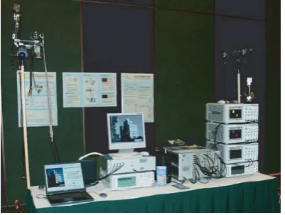
The real-time MIMO test-bed described here was developed in the GermanHyEff project. The goal was to show the feasi-bility of MIMO in real-time in a single-carrier link based on the well-known flat-fading algorithms, and to speed up the signal processing in this first step beyond the natural limits set by the temporal dispersion found in typical indoor chan-nels. We evaluated various architectures and implemented one promising approach which is fully operational since July 2003 (seeFigure 1). This prototype has been presented with real-time transmission experiments at the Globecom confer-ence in San Francisco in December 2003.
Figure1: Real-time MIMO test-bed at a presentation at Globecom 2003.
3.1. General concept of the multiantenna test-bed
To exploit the multiplexing and diversity potential of mul-tiantenna systems, a higher effort of baseband signal pro-cessing is a prerequisite. To match those signal propro-cessing re-quirements, a hybrid design was chosen for the test-bed (see
Figure 2). The main baseband signal processing units con-sist of an FPGA for very fast matrix vector multiplications and a DSP for a flexible implementation of more sophisti-cated algorithms. This baseband design concept unites real-time high-data-rate capability and a high flexibility regarding the detection and precoding algorithms under investigation. The D/A and A/D converters use duplex mode2and are in-tegrated on a special board which is plugged onto the FPGA board.
The RF frontend uses direct up- and downconversion (DUC/DDC) and uses a center frequency of 5.2 GHz for the local oscillator (LO).
3.2. Description of the transmitter and
receiver—RF chains, DAC, and ADC
3.2.1. Transmitter
In the setup under investigation, we use four transmit anten-nas. The 5.2 GHz radio hardware has a bandwidth of roughly 100 MHz and it performs direct analog upconversion using four I/Q mixers each followed by +20 dBm power amplifier (ZRON-8G, Mini Circuits); seeFigure 3.
Up to four independent complex-valued data streams are transmitted over the air. The data generation and the mod-ulation are realized within a Xilinx Virtex II 8000 FPGA. The output signals are D/A converted with 12-bit resolution and used to modulate the carrier. One reason to use FPGAs
2Duplex mode refers to synchronized parallel sampling of two inputs, for example, I and Q and a followed serial mapping for read/write operations on the bus to the FPGA. Therefore, the bit width of the bus can be re-duced.
instead of DSPs is the need for a joint signal processing of multiple data streams. The limited number of in- and output ports of current DSPs may not allow multiple high-data-rate streams in parallel. Due to the FPGA realization, all the sig-nal processing must be carefully programmed in VHDL to allow a proper timing control. The periodically transmitted signal consists of a preamble and a data block. Each I and Q branch of the Tx antennas is tagged with a different 127-bit Gold sequence transmitted in BPSK format in a preamble. The length of the pilots is intentionally oversized in the ex-perimental system to get precise channel estimates. The pi-lots are followed by a pseudorandom data block with 1024 symbols on each stream. The modulation of the data is in-dependently set on each I and Q branch with up to 16 PAM levels allowing schemes from BPSK to 256-QAM.
3.2.2. Receiver
The received signals from 5 antennas are directly downcon-verted using analog I/Q demodulators and digitized using 12-bit AD converters (seeFigure 4).
The analog design creates a severe I/Q imbalance (3–4 degrees for commercial I/Q mixers) which has to be taken into account in the entire system concept. In principle, we treat the complex-valued MIMO baseband system with 4 Txs and 5 Rxs as a real-valued system having 8 Txs and 10 Rxs to compensate the I/Q crosstalk.
Note, that the I/Q imbalance can be compensated at each transmit and receive antenna after a careful calibration is done. This is of ever greater importance for OFDM schemes [58] due to the crosstalk between the image frequencies. For the SISO-OFDM case [59–61] proposed the estimation of the IQ imbalances based on statistical measures but these con-cepts are not applicable straightforward for multiple anten-nas since signals coming from different transmit antennas are not separable by the this method. Therefore, our concept of realvalued data separation can be used here as well but now the symbols on subcarrier fihave to be reconstructed
together with the symbols from subcarrier−fi [62] which
expands the detector matrix, for example, MMSE filter by a factor of 2 in each dimension. For a MIMO-OFDM system with 4 Tx and 5 Rx antennas, this would mean that a real-valued matrix with 2(2nT)×2(2mR)=320 entries had to be
computed and processed in real time with the received data vector. In case that the number of multipliers in the FPGA is limited, then an I/Q preequalization at the Tx antennas and an I/Q equalization at the Rx antennas is a reasonable alter-native, but careful calibration is needed in advance. For low signal bandwidth (<50 MHz), digital up- and downconver-sion is another favorable option.
3.3. FPGAs—for high speed parallel signal processing
3.3.1. Channel estimation
Tx FPGA transmitter with parallel M-PAM data source sends training piolts, adapts modulation; preprocesses data for SVD-MIMO or
adaptive channel inversion D/A D/A D/A Data 1 Data 2
Datak−1
Datak . . . . . . . . . . . . . . . . . . I/Q-mod I/Q-mod I/Q-mod MIMO channel I/Q-demod I/Q-demod I/Q-demod I1 Q1 IM QM A/D A/D A/D Rx FPGA performs channel estimation; separates parallel data
streams by matrix multiplication or simply
scales received data; demodulates M-PAM;
performs bit- and block-error-rate measurement for all
data streams
D/A
D/A
D/A
Channel
estimation (H) Weights (W)
d1
d2
dk−1
dk . . . . . . . . . . .
. Reco
n st ru ct ed d at a DSP
calculates weights for linear MMSE receiver & controls link adaptation and bit loading; calculates linear precoding matrices for the
transmitter Bit loading & Tx-weights
Figure2: Principle of the real-time MIMO test-bed.
D/A D/A I Q Analog IQ modulator
5.2 GHz
+20 dB ZRON
PA
Figure3: Baseband to RF transmitter chain.
next bit in the sequence may eventually change the sign of the signal to be accumulated, so the CC switches from addition and subtraction. Additional CCs based on unused sequences are used to estimate the noise variance of each receive branch. The channel estimates are immediately available after the last bit in the training sequence and stored in dedicated regis-ters. These registers are read out by a separate DSP (Texas Instruments 6713) connected to the FPGA via a parallel bus (24- bit flat ribbon cable). The DSP is used to calculate the coefficients of, for example, a linear MMSE filter which are then sent back to the dedicated weight registers in the FPGA via the same link. The read and write operations of the DSP are fully asynchronous to the transmitted frame structure.
3.3.2. MIMO detection
Two linear detection schemes, ZF and MMSE, were imple-mented in the Rx-FPGA as a matrix-vector multiplication unit to separate the spatially multiplexed data streams. Note that for a 4×5 MIMO system, this unit consumes 80 dedi-cated multipliers, which sets an upper limit to the numbers of antennas depending on the FPGA size (Virtex II, Virtex II Pro 70/100, etc.). If a matrix-vector multiplication of big-ger size has to be performed, then, for example, a rowwise multiplication of H†·y can help to overcome the limited
number of multiplier units where H† denotes the MMSE pseudoinverse of the channel andydenotes the receive vec-tor.
For nonlinear detection like SIC and V-BLAST a deci-sion feedback equalizer (DFE) structure3was implemented. The feedforward matrix GFuses the same matrix block as for the linear equalization. After each symbol decision, the decided symbols are fed back by a multiplication with a tri-angular feedback matrixB−I. The DFE design was imple-mented such that for the detection of one symbol vector, the DFE loop is passed several times until the last element of the symbol vector is detected. With 8 real-valued data streams, the maximum symbol rate of this DFE design is limited to 1 MSymbol/s, due to 25 MHz FPGA system clock, which was the FPGA clock rate for the flat-fading design at the time of the implementation. In principle, this was sufficient for sym-bol rates up to 10 MHz due to the measured temporal dis-persion in our lab. A way out to support higher symbol rates with SIC the DFE detection unit can be run at a higher sys-tem clock rate (100–150 MHz) or the structure can be set up in parallel at the cost of more multiplication units.
The DFE design inFigure 5allows a fair comparison of several detection schemes by simply loading different matri-ces for the feedback and feedforward filters, for example, for ZF and MMSE, the feedback matrixB−Iis loaded with zeros.
3.3.3. MIMO precoding
Several MIMO transmission schemes like SVD-MIMO or joint transmission/linear channel inversion require spatial precoding at the transmitter. The spatial precoding was im-plemented in the Tx-FPGA after the parallel PAM
AD AD I
Q Analog IQ demodulator
5.2 GHz +20 dB
+20 dB +7. . .+ 27 dB
Low noise amplifier
Digital interface
Figure4: RF to baseband receive chain.
2nt
Correlator for MIMO channel estimation 2mR
18bits
2×mr 2×nt ⎡
⎣HZF+/HMMSE’+
G.F, UHST
⎤ ⎦
12bits
A/D oDC-ffset A/D oDC-ffset
1 Q
I
12bits 12bits
5 IQ
28bits
2
.nT
+ −
12bits
PAM-detect 12bits
PAM DEMOD
8bi ts
[B−I]
12bits
BER/ FER
8bi ts
PRBS-generator
8bi ts
DSP
Figure5: Block diagram of DFE structure inside the Rx-FPGA with channel estimation, MIMO detector (DFE), a demodulator, and a BER/FER unit.
tion block with a matrix multiplication unit similar to that from the Rx but using only 64 dedicated multipliers. The ma-trix entries are calculated by the DSP as well and loaded via the 24- bit DSP-FPGA parallel bus at the time of the experi-ments. While this paper is written, the test-bed is equipped with reciprocal transceivers proposed in [63], such that the spatial precoding can be calculated by the Tx independently, relying on a channel estimation in the opposite direction in TDD mode.
3.3.4. Demodulation
The separated streams are demodulated using hard decisions in each I- and Q-branch.
The temporal dispersion in the multipath indoor chan-nel obviously sets the upper limit to the maximal symbol rate, which was 10 Msymbols/s in our lab. Using symbol rates of 5 Msymbols/s, this corresponds to an overall data rate of 40 Mbps with QPSK and 120 Mbps with 64-QAM modula-tion on all four Tx antennas (8 bps/Hz and 24 bp/Hz).
Therefore, the current bandwidth extension to 100 MHz required multicarrier techniques (OFDM).
The signal processing itself can support even higher rates and more complex schemes like, for example, MIMO-OFDM which has been implemented on the reconfigurable signal processing platform, recently.
3.3.5. Bit error rate measurements
The BER measurement is performed automatically on all data streams based on a comparison of the separated and demodulated signals at the Rx and the data coming from the PRBS-data generator are also programmed inside the Rx-FPGA. The error measurement is performed on bit and frame level as well and can be file-logged on the PC.
3.3.6. Synchronization
Since the channel impulse response causes spikes with ex-ponential decay when changing from symbol to symbol, the symbols are sampled at about 70% to 80% of its length. By this adjustment, a reliable channel measurement could be achieved up to symbol rates of 10 Msymbols/s.
Synchronization over the air is currently being imple-mented for MIMO-OFDM but was not finalized at the time when the experiments were conducted with the single-carrier setup.
3.4. DSPs—exploiting flexibility
3.4.1. Channel tracking
With respect to higher mobility, it becomes critical to track the MIMO channel sufficiently fast. The most challenging part becomes the weight calculation when there are a few dozens of OFDM carriers and for each of them a weight ma-trix has to be calculated. Appropriate algorithms for the im-plementation on a DSP are discussed inSection 4.6. If those weights are available within one or a few milliseconds,4 chan-nel tracking is expected to be fast enough for indoor and pedestrian applications. For higher mobility, channel track-ing within each frame becomes mandatory.
3.4.2. Bit loading or rate control
It is calculated at the Rx. The DSP calculates the actual possi-ble PAM constellation based on the expected noise enhance-ment after the MIMO detector. This is equivalent to the SINR in front of the demodulator. Here, the I/Q imbalances causes different noise enhancement in I and Q (see alsoFigure 14). Therefore, we control the modulation independently for the I- and Q-part of each symbol by using PAM instead of M-QAM. This higher channel adaptivity translates directly into a higher throughput and link reliability.
3.4.3. Feedback link
Based on the channel estimates, the DSP may calculate the optimal modulation in each stream. Note that the test-bed is currently operational only in simplex mode. So the loading vector is sent back to the Tx-FPGA via a parallel bus, thus realizing an ideal feedback link.
4. MIMO ALGORITHMS AND OPTIMIZATION
4.1. Basic algorithmic strategies for real-time
multiantenna systems with high data rates
With the perspective of real-time capable algorithm im-plementation for very high data rates, the complexity of
4The current frame size of 2 milliseconds matches well with the frame structure of commercial WLAN systems (IEEE 802.11a/b/g).
algorithms often becomes a limiting factor. Therefore, it is reasonable to search for solutions which have a high perfor-mance and match the capability of a dedicated hardware.
The hybrid FPGA/DSP architecture of the test-bed gives a high flexibility over algorithms used for data stream sepa-ration at the Tx and/or the Rx, rate and power control. Those algorithms are run on the DSP while the fixed part (e.g., channel estimation, data separation, mod/demod, BER) is performed by the FPGA. The DSP works fully asynchronous and refreshes, for example, the necessary MMSE weights and/or the bit-loading vector at the Tx-FPGA within a mil-lisecond or less.
Following this divide-and-rule strategy, we are able to support high data rates in a MIMO transmission and still have the flexibility towards algorithms.
To realize this ambitious approach, we implemented the high-speed matrix-vector multiplications for the reconstruc-tion of the data streams in VHDL on the FPGA and the DSP performs the calculation of the required matrices. The com-plexity which can be implemented in the FPGA is mainly limited by the number of dedicated multipliers, RAM, and so forth, and particularly by the maximum clock rate at which the design can be routed within the required de-lay limits. The more resources are used from the FPGA (70% or more), the more difficult the place & route pro-cedure becomes. The limiting factor for high-speed signal processing in the FPGA is determined by the ADC, DAC, and FFT/IFFT blocks (e.g., OFDM) which run at the high-est clock rates which is limited to 150–200 MHz in reality (Virtex II Pro 100), which limits the usable signal band-width to be used for transmission. This means that for high data rates of several 100 Mbps to 1 Gbps or more, higher modulation levels and spatial multiplexing are a ne-cessity.
A recent FPGA implementation of MIMO-OFDM at a clock rate of 100 MHz [64] has allowed a reliable low-mobility transmission with a gross data rate of 1 Gbps with 3 Tx and 5 Rx antennas using 48 active OFDM carriers and 100 MHz bandwidth at 5.2 GHz.
can be exploited to reduce the MIMO signal processing sig-nificantly. A promising approach is the calculation of an ex-act solution (e.g., ZF-pseudoinverse as proposed by [65]) on (L−1)(NT −1) + 1 subcarriers only and to interpolate the
filter solutions in between.5If this is done in an appropriate trigonometrical fashion [66], the interpolated filter matrices can reconstruct the multiplexed data streams with high ac-curacy. The savings in time for the calculation of the MMSE solutions have to be traded carefully against the additional effort for the interpolation.
MIMO transmission schemes require specific algebraic procedures to be performed in order to precode or de-code the data appropriately. Some useful algorithms are dis-cussed in the following paragraphs. Most of them were im-plemented on the DSP in C language and used for the calcu-lation of the MIMO filter matrices in the transmission exper-iments.
4.2. DSP—architecture and optimization
One of the initial decisions which has to be taken is between floating-point and fixed-point arithmetic. Fixed-point DSPs are offered on the market at much higher clock rates (e.g., 1 GHz) than floating-point DSPs (300 Mhz), so one might say let us take the faster one. But this is only true if all calcu-lations are performed in the integer domain and the dynamic range is fixed and well known. If floating types like float or double are used, the mapping to integer numbers is per-formed automatically by the compiler. A simple test showed that, for example, a matrix inversion on a 16-bit fixed-point TI-DSP (1 GHz) performs slower than the 300 MHz 32-bit floating-point DSP (TI6713) by a factor of 10. A way out is to optimize the mapping by hand using additional knowledge about the dynamic range, and so forth. A major drawback of this approach is that hand-optimized program code is hard to read and therefore very error-prone and not very flexible to code changes, not to mention a lot of overhead may occur when different people are contributing to the same algorithm library without necessarily knowing all details on dynamic range of the possible input and output values. Furthermore, assembly code optimization is more difficult on a fixed point target.
Therefore, we choose the floating-point architecture (TI6713) with 225 MHz for the test-bed to have as much al-gorithmic flexibility as possible.
Reference [67] investigated several MIMO algorithms in great detail regarding general C-code and assembly optimiza-tion. We will limit ourselves to the performance results in
Section 4.6.
5The classical approach of interpolation of the frequency channel estimates by a transfer into time domain, appropriate windowing, and a back trans-formation to the required number of subcarriers in the frequency domain improves the accuracy of the channel estimation but does not help to re-duce the calculation effort at all. Note that the filter envelopes of analogue or digital filters which are used for image band suppression have to be measured carefully before interpolation techniques can be exploited. This is important in particular when more than 80% of the OFDM subcarriers are used, which can be done with channel adaptive bit loading.
4.3. Matrix inversion and decompositions
Many MIMO precoding and reception techniques are based on matrix-vector multiplications either in a linear sense or a nonlinear sense which means repeating matrix-vector oper-ations with decisions in between. The required matrices are mostly obtained by matrix decompositions or matrix inver-sions, so we will focus on those very important algebraic al-gorithms. Since real-time capability is mandatory for high-data-rate MIMO applications, speed and numerical stability are of great importance. Another aspect is fixed or variable computational time, since in many applications it is not the average computation time which matters but very often the worst-case time. Therefore, a fixed computation time is de-sirable and often easier to optimize.
4.4. The inverse of a matrix and the pseudoinverse
By definition, the inverse of a matrix only exists for matrices with the same number of rows and columns. LetAbe a ma-trix of sizemR×nT withmR =nT. Then we defineA−1the
inverse of matrixAif it holds that
InT=AA
−1=A−1A, (1)
whereInTis the unity matrix of sizenT×nT.
IfAis of rectangular shapemR×nTwithmR ≥nT, then
an inverse is not defined. Therefore, a so-called pseudoin-verse has to be computed instead:
A†=AHA−1AH, (2)
where (AHA)−1has square shape and standard algorithms for matrix inversion are applicable.A†then satisfiesInT =A†A
similar like in (1). When using (·)†in the following, we will refer to the Moore-Penrose pseudoinverse which causes low-est noise enhancement when multiplied with the receive vec-tor.
In multiple-antenna systems, the signals coming from all Tx antennas are superimposed at the Rx antennas. For the separation of these signals, for example, a linear filter can be used. A simple realization can be achieved with a zero-forcing (ZF) filter while the minimum mean-square error (MMSE) is more complex but considers the noise from the Rx and outperforms ZF regarding the BER especially in the low SNR region. Both solutions require one matrix inversion each.
A linear equalization at the Rx corresponds to a multipli-cation of the receive vectorywith a matrixH†. The trans-mitted data can then be estimated as
x=H†y=H†Hx+H†n=x+H†n, (3)
where the ZF-pseudoinverse ofHformR≥nTis
H†ZF =HHH−1HH, (4)
or if we consider the receiver noise, additionally, the belong-ing MMSE filter reads
H†MMSE=HHHHH+σ2
NI
−1
where the noise varianceσN2 is assumed to be the same for all
receivers for a more convenient notation. Note that in gen-eral we have to expect different noise variances for each re-ceiver if, for example, independent automatic gain controls are used.
4.5. Calculation of the inverse/pseudoinverse
One straightforward approach to implement the calculation of the inverse and/or pseudoinverse is usingGreville’s method [68]. This algorithm provides full flexibility in the number of Tx and Rx antennas and even some columns or rows can contain zero vectors.
While the ZF filter from (4) can be calculated directly fromHinstead of invertingHHH, the MMSE filter from (5)
requires two extra matrix multiplications and the inversion of (HHH+σ2
NI) which is of sizemR×mR.
Keeping in mind that the computational effort of mul-tiplications and inversions increases by ∼ N3 with N = max(nT,mR), we can choose a dimension-reduced
formula-tion of the MMSE for the implementaformula-tion:
reduced MMSE:H†MMSE=
HHH+σN2I
−1
HH, (6)
whereσ2
Nis now equivalent noise variance per data stream.
Furthermore, the range of the data is an important issue in the conjunction with algorithms to calculate a pseudoin-verse, since a calculation ofHHHdoubles the binary range
from, for example, 12 bits to 24 bits which can decrease the algorithmic stability. In other words, the condition number6 of the matrix to be inverted is increased by a power of two whenHHHis inverted instead ofH. This range extension is
not required when Greville’s method is used, so this may be an algorithm of choice for fixed-point implementation.
Another algorithm which can be used is based on a mod-ification of the Frobenius formula [68] where the calculation of a pseudoinverse can be performed by the calculation of pseudoinverses of submatrices:
A B C D
−1
=
K−1 −K−1BD−1
−D−1CK−1 D−1+D−1CK−1BD−1
, (7)
whereK =A−BD−1C. If the submatrices of theFrobenius decompositionare regular and of square shape (e.g.,A), then inversion can be performed by calculating the elements of the inverse matrixA−1directly with Cramer’s rule
a(ik−1)= Aki
A. (8)
The implementation of (8) is quite straightforward up to a matrix size of 4×4 real-values. For instance, if the matrixH
is of size 6×6 or 8×8, then a decomposition into 3×3 or 4×4 submatrices is advised, respectively. Note that the calculation
6The condition number is used here as the fraction of the biggest and the smallest singular value of a matrix.
of a matrix inverse with Cramer’s rule (8) is not advised with regard to numerical stability due to the determinant in the denominator.
For the special case of the inversion of a square matrix with full rank, which is true for the MMSE solution with nonzero noise in (5) and (6), there is another option to ob-tain a matrix inverse. Following the outline of [69], Gauss-Jordan eliminationhas the advantage of a high numerical sta-bility, especially when full pivoting is used. Furthermore, the structure of the algorithm allows a very efficient manual op-timization of the C-code.
Beside the three given examples, many more algorithms were optimized, implemented, and evaluated towards nu-merical stability and speed. An short overview including QR and QL decomposition is given inFigure 6.
4.6. Performance analysis
To evaluate and compare algorithms, we have to characterize the complexity or the computationally required effort. Very often the measure is given in flops (floating-point opera-tions), where the definitions are varying among different au-thors. Instead we will compare all algorithms by the amount of required multiplications. Since additions mostly occur in pairs with multiplications, we only have to count the latter.
Reciprocal values (1/X), square roots (√X), and recipro-cal square roots (1/√X) are counted separately, since their computation needs more cycles on the DSP. In the algorith-mic optimization process, the minimization of those opera-tions has a high priority. Unavoidable divisions will always be replaced by reciprocal values. All algorithms are used on matrices of sizem×nand
mn3+n2, n 1
X, n
1
√
X (9)
denotes an algorithms consisting ofmn3+n2multiplications (additions), nreciprocal values, and n reciprocal roots. In
Table 1, the complexity of several algorithms is summarized.
Figure 7 illustrates a complexity comparison of typi-cal linear (Figures 7(a),7(b)) and nonlinear (Figures7(c),
7(d)) MIMO algorithms based on real multiplications. It is clearly to be seen that complex calculations7 (Figures7(b),
7(d)) reduce the complexity significantly but can only be ex-ploited when the I/Q-imbalance is negligible. On the other hand, real-valued SIC detection offers exploitable perfor-mance gains even without I/Q-imbalance as shown in [70]. InFigure 7(c), we can see that the classical V-BLAST algo-rithm (solid triangles) based on ZF- or MMSE-matrix in-versions, which is in principle anO(N4) algorithm, will be
MIMO-detection schemes Linear
ZF
#transmitter=#receiver Inverse (I)
LU-decomposition (LUD) Crout
Doolittle Gauss-algorithm Inverse (I)
Gauss-Jordan (GJ)
LU-decomposition + forward-and backsubstitution Gauss-algorithm + backsubstitution
#transmitter#receiver Pseudoinverse (PI)
Moore-Penrose (MP)
Gauss-Jorden for symmetric. Positive definite matrices (GJsym) + matrix multiplication. (Symmetric) + matrix multiplication
Choleski-decomposition + forward-and backsubstitution + matrix multiplication. (Symmetric) + matrix multiplication Greville
MMSE
#transmitter#receiver Pseudoinverse (PI)
Moore-Penrose (MP), see above With QR-decomposition (QRD)
Gram-Schmidt-QRD + matrix multiplication (triangular matrix) Nonlinear
SIC ZF
QR-decomposition (QRD) Householder (Ho) Gram-Schmidt (GS) MMSE
QR-decomposition (QRD) Householder (Ho) Gram-Schmidt (GS) V-BLAST
ZF
With pseudoinverse (PI)
Moore-Penrose (MP), see above With QR-decomposition (QRD)
Householder-QRD + inverse (triangular matrix) MMSE
With pseudoinverse (PI)
Moore-Penrose (MP), see above With QR-Decomposition (QRD)
Gram-Schmidt-QRD + inverse (triangular matrix)
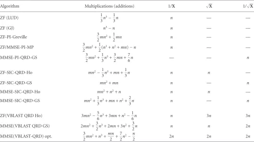
Table1
Algorithm Multiplications (additions) 1/X √X 1/√X
ZF (LUD) 1
3n 3−1
3n n — —
ZF (GJ) n3−n n — —
ZF-PI-Greville 3
2mn 2+1
2mn n — —
ZF/MMSE-PI-MP 3
2mn 2+1
2(n
3+n2+mn)−n n — —
MMSE-PI-QRD-GS 3
2mn 2+1
3n 3+3
2mn+ 7
6n — — n
ZF-SIC-QRD-Ho mn2−1
3n
3+mn+1
3n n n —
ZF-SIC-QRD-GS mn2+mn n — n
MMSE-SIC-QRD-Ho mn2+n2+n n n —
MMSE-SIC-QRD-GS mn2+1
3n
3+mn+n2+2
3n n — n
ZF(VBLAST QRD Ho) 3mn2−5
6n
3+ 3mn+n2−1
6n n 3n 3n
MMSE(VBLAST QRD GS) 2mn2+3
2n
3+ 2mn+ 3n2+3
2n n n 2n
MMSE(VBLAST-QRD) opt. 3
2mn
2+n3+mn 2 +
7 2n
2−n
2 2n 2n 2n
outperformed by the QRD pre and postsort approach (bul-lets) proposed by [71] only for large numbers of antennas N ≥ 10 when a complex calculation would be performed. For the real-valued signal processing, a comparable complex-ity is achieved at about 6 Tx and Rx antennas. So the com-putational gain is more to be seen in a sense that the post-sorting algorithm has to be run only when the detection or-der has to be tracked permanently, for example, with fixed-rate transmission. In case of adaptive bit loading, the detec-tion order is only once computed for every bit-loading pro-cedure and is then held fixed till the next bit loading, hence most of the time QRD is sufficient for tracking the channel. Therefore, the additional expenses for the V-BLAST ordering now and then are less burden to the time budget.
So by carefully counting all necessary operations, a prin-ciple performance prediction with, for example, rising ma-trix size can be given. An implementation of the algorithms on a DSP might give different results since every dedi-cated DSP architecture supports some algorithmic structures better than others. Therefore, the experienced programmer matches the algorithm implementation to the computational strength of a specific DSP type. Still limitations like a certain number of possible parallel assembly instructions or a lim-ited cache size can cause that even slight changes in the code (e.g., loop length or matrix size) can change the number of required cycles significantly.
Figure 8 shows algorithm speed implemented on the TI6713 DSP for single-carrier systemFigure 8(a)andFigure 8(b)and an OFDM system where 48 subcarriersFigure 8(c)
andFigure 8(d)are active, hence 48 channel matrices have to be inverted. Several linear detection algorithms are de-picted inFigure 8(a)andFigure 8(c)whileFigure 8(b) and
Figure 8(d)show the performance of some algorithms used for nonlinear detection. All algorithms are performed with real-valued calculation. For a 48-subcarrier OFDM, the run time exceeds the 1-millisecond (indoor environment) level already for small numbers of antennas (N <6) even for the linear schemes. This shows that further acceleration includ-ing assembly programminclud-ing, multiple DSP, and/or interpola-tion techniques is inevitable.
The black square inFigure 8(a) andFigure 8(c)depicts the performance which was achieved with an exemplary as-sembly code optimization for 2 Tx and 2 Rx antennas (4×4 real-valued matrix). This measurement together with an as-sembly design for an 8×8 real-valued matrix was used to pre-dict the assembler performance for some MIMO algorithms. The estimated run-times (in microseconds) for an OFDM system with 48 subcarriers are collected inTable 2.
10 100 1000 10 000
N
u
mber
of
re
al
m
ultiplications
2 4 6 8 10 12 14 16 Number of antennasnT=mR
ZF-inverse (LU-decomposition) ZF-inverse (Gauss-Jordan- inversion) ZF-pseudoinverse (Greville)
MMSE-pseudoinverse (Moore-Penrose) (a)
10 100 1000 10 000
N
u
mber
of
re
al
m
ultiplications
2 4 6 8 10 12 14 16 Number of antennasnT=mR
ZF-inverse (LU-decomposition) ZF-inverse (Gauss-Jordan- inversion) ZF-pseudoinverse (Greville)
MMSE-pseudoinverse (Moore-Penrose) (b)
10 100 1000 10 000 100 000
N
u
mber
of
re
al
m
ultiplications
2 4 6 8 10 12 14 16 Number of antennasnT=mR
ZF-MMSE-V-BLAST (pseudoinverse) MMSE-V-BLAST (GS-QRD)
MMSE-V-BLAST (GS-QRD) optimized MMSE-SIC (GS-QRD)
ZF-V-BLAST (housholder-QRD) ZF-SIC (householder-QRD)
(c)
10 100 1000 10 000 100 000
N
u
mber
of
re
al
m
ultiplications
2 4 6 8 10 12 14 16 Number of antennasnT=mR
ZF-MMSE-V-BLAST (pseudoinverse) MMSE-V-BLAST (GS-QRD)
MMSE-V-BLAST (GS-QRD) optimized MMSE-SIC (GS-QRD)
ZF-V-BLAST (housholder-QRD) ZF-SIC (householder-QRD)
(d)
Figure7: Computational complexity of several algorithms used for linear (a)–(b) and (c)–(d) nonlinear MIMO processing. (a)–(c) Matrices are real-valued; (b)–(d) matrices are complex-valued. All multiplications are counted as real-valued multiplications.
in one DSP. Nonlinear detection seems to be feasible with up to 6×6 antennas without optimum ordering. If addition-ally a V-BLAST ordering is required for every filter, then the matrix size is limited to a 4×4 antenna configuration.
The MIMO-OFDM configurations with higher antenna numbers can be supported with one TI6713 DSP only when the channel coherence time is much longer (quasistatic sce-narios) or alternatively a DSP cluster must be used to parti-tion the calculaparti-tion effort subcarrier-wise and work in paral-lel.
5. REAL-TIME MIMO TRANSMISSION EXPERIMENTS
5.1. Transmit and receive configurations
1 10 100
Ti
m
e
(
μ
s)
2 4 6 8
Number of antennasnT=mR
Assembler Greville
ZF-inverse (Gauss-Jordan- w/o pivot.) ZF-inverse (Gauss-Jordan- with pivot.) ZF-pseudoinverse (Greville)
MMSE-pseudoinverse (Moore-Penrose) (a)
1 10 100
Ti
m
e
(
μ
s)
2 4 6 8
Number of antennasnT=mR
ZF-SIC (Gram-Schmidt-QLD) MMSE-SIC (Gram-Schmidt-QLD) ZF/MMSE V-BLAST (pseudoinverse) MMSE-V-BLAST (Gram-Schmidt-QLD)
(b)
100 1000 10 000
Ti
m
e
(
μ
s)
2 4 6 8
Number of antennasnT=mR
Assembler Greville
ZF-inverse (Gauss-Jordan- w/o pivot.) ZF-inverse (Gauss-Jordan- with pivot.) ZF-pseudoinverse (Greville)
MMSE-pseudoinverse (Moore-Penrose) Wiener filter
(c)
100 1000 10 000
Ti
m
e
(
μ
s)
2 4 6 8
Number of antennasnT=mR
ZF-SIC (Gram-Schmidt-QLD) MMSE-SIC (Gram-Schmidt-QLD) ZF/MMSE-V-BLAST (pseudoinverse) MMSE-V-BLAST (Gram-Schmidt-QLD) Wiener filter
(d)
Figure8: Measured cycles on TI6713 DSP displayed in microseconds for (a)–(c) linear and (b)–(d) nonlinear MIMO algorithms. (a)–(b) Single-carrier system; (c)–(d) OFDM system with 48 active subcarriers.
simply do always the same straightforward matrix-vector multiplications with the actually loaded solutions from the DSP.
To bring more transparency into all possible transmit and receive configurations,Table 3will help. The table has to be read in the following way. The first column gives the trans-mission scheme under investigation and the belonging up-link (UP) or downup-link (DL) scenario where it can be ap-plied to. The next two columns contain the matrices which
Table2
Number of antennasnT=mR
2 3 4 5 6 8
ZF-I-LUD 25 48 86 140 220 460
ZF-I-GJ 36 88 180 330 550 1200
ZF-PI-Gr 49 130 270 490 820 900
MMSE-PI-MP 90 160 350 640 1100 2500
MMSE-PI-QRD-GS 66 170 360 660 1100 2400
ZF-SIC-QRD-Ho 55 110 190 310 480 1000
MMSE-SIC-QRD-GS 53 130 270 490 800 1800
ZF/MMSE-VBLAST-PI 86 240 540 1000 1800 4700
ZF-VBLAST-QRD-Ho 170 350 620 1000 1600 3300
MMSE(VBLAST QRD GS) 140 310 600 1000 1600 3500
Table3
Transmission scheme Transmit processing Receive processing Modulation alphabet Bitloading parameter
PARC (UL) I ZF/MMSE:H†
SIC:GF,B−I
Mod per antenna 0-/2-/4-/8-/16-PAM
diag(H†·H†T)
(diag(L))−2(QLD)
SVD-MIMO (UL/DL) V UT·D−1 Mod per data stream
0-/2-/4-/8-/16-PAM
diag(D−2) (SVD)
ACI/JT (DL) H†/α α·I Same mod for
all active streams 0-/2-/4-/8-PAM
α2from 12-bit-DAC scaling
Multiuser scheduling (UL) I ZF/MMSE:H† Mod per user
0-/2-/4-/8-PAM
diag(H†·H†T)
5.2. Adaptive transmission schemes—flat fading
The transmission schemes summarized inTable 3were im-plemented on the MIMO test-bed with a single carrier at 5.2 GHz, data symbol rates from 1 Msymbol/s to 10 Msymbols/s and adaptive modulation from 2–16 PAM which equals 256 QAM as highest modulation scheme. The detailed exper-imental results are published in [18,49,55,72].
Beside one extra antenna at the Rx channel, adaptive bit loading was an essential part to make the MIMO link much more stable and reliable since transmission over bad channels was avoided. It was found during the experiments that chan-nel tracking and bit loading or multiuser scheduling can be performed at different time scales, since a change in the chan-nel first causes phase and amplitude changes but the SINR behind a MIMO detector is changing much slower. Keeping in mind that switching from one QAM-level to the next or backwards requires about 6 dB more or less SINR, it can be easily understood that bit loading can be run on another time scale. During all our measurements, the Rx antenna set was moving with 4 cm/s along a 5- meter long railway-like con-struction, so channel tracking within one millisecond was sufficient while bit-loading could be done about every 100 milliseconds without losing throughput or violating the av-erage BER target.
The reproducibility of channel realizations by moving the Rx antennas always the same path through the room was a key issue to compare various transmission and detection schemes. As discussed in [49], the measured channel statis-tics in the laboratory seen from the pdf of the singular values behaves very similar to an i.i.d. Rayleigh channel with a slight Rician component. Furthermore, the deteriorating effect of I/Q imbalances was reported to be seen in a split-up of the singular values which should be pairwise degenerated oth-erwise [49]. This also underlines that real-valued baseband signal processing is a good option with direct analogue up-and downconversion as used in the test-bed.
Due to the similarity of the channel, in our lab with an i.i.d. Rayleigh channel we could measure the MIMO diver-sity slopes (dotted lines) inFigure 9in very good accordance with what was expected from theory under the assumption of uncoded fixed modulation transmission and a linear de-tector. The average SNR per Rx antenna was calculated indi-rectly from the measured channel along the track.
Throughput experiments with several MIMO transmis-sion schemes combined with channel adaptive bit loading as described in [49] were conducted. The results are summa-rized in Figures10and11.
1E−5 1E−4 1E−3 0.01
0.1
Av
er
ag
e
B
E
R
30 25 20 15 10 5 0 Attenuation at all Tx antennas (dB)
−2 13 28
Average SNR per Rx antenna (dB)
4Tx 4Rx 4Tx 5Rx
3Tx 5Rx 2Tx 5Rx (a)
1E−5 1E−4 1E−3 0.01
0.1
Av
er
ag
e
B
E
R
40 30 20 10 0
Attenuation at all Tx antennas (dB)
−12 8 28
Average SNR per Rx antenna (dB)
4Tx 1Rx 4Tx 2Rx
4Tx 3Rx 4Tx 4Rx (b)
Figure9: Uncoded BERs for various Tx/Rx configurations in the lab. (a) ZF detection in the uplink, (b) joint transmission in the downlink.
0 5 10 15 20 25
Av
er
ag
e
sp
ec
tr
al
e
ffi
ciency
(bps/Hz)
20 15 10 5 0
Attenuation at all Tx (dB)
8 18 28
Average SNR per Rx antenna (dB)
Linear MMSE MMSE-SIC SVD-MIMO
SVD-MIMO 64QAM cutoff MMSE-SIC 64QAM cutoff Modulation: QPSK/16−/64−/256−QAM
symbol rate : 1 MHz targeted average BER=10−2
Figure10: Comparison of the achieved average sum rate with 4 Tx and 5 Rx antennas with linear MMSE or MMSE-SIC and SVD-eigenvalue transmission in real-time experiments.
(upper curve), MMSE-VBLAST at Rx (middle), and linear MMSE at Rx (lower curve). At very low SNR the latter two schemes achieve similar low throughput which can be ex-plained that with both schemes most of the time only one or two data streams are switched on and SIC can not gain much. At high SNR SIC gains up to 3- bit additional throughput compared to the linear MMSE due to the SINR increase for later detected layers. The SVD scheme outperforms the other
0 0.2 0.4 0.6 0.8 1
Empir
ical
cd
f
6 8 10 12 14 16 18 20 22 24 26 28 30 Spectral efficiency (bps/Hz)
SVD-MIMO MMSE-SIC MMSE
Attenuation at all antennas 0 dB Symbol rate : 1 MHz QPSK, 16−/64−/256−QAM
Targeted average BER=10−2
Figure 11: Empirical cdf of the achieved average sum rate with 4 Tx and 5 Rx antennas with linear MMSE, MMSE-SIC, and SVD-MIMO transmission. Attenuation at all Tx antennas =0 dB (ap-prox. 28 dB SNR per Rx antenna).
Since we perform adaptive bit loading in such a manner that all layers meet a certain BER target, we have to consider the effect of error propagation in the bit-loading algorithm. The weaker the BER decay (diversity slope), the more extra trans-mit power necessary to fulfill the target. As an example let us assume a BER target of 10−3for all layers. Since all layers including the last layer will meet this BER target, we have to set the BER target for each layer lower such that including er-ror propagation we will satisfy the targeted BER. Assuming 4 Tx and 5 Rx antennas and a multiplexing of 4 data streams, we can expect a BER diversity order∼ SNR−2. If we had a 100% error propagation, then as a rule of thumb the last layer would suffer from 3/4 of possibly propagated errors and 1/4 of own decision errors meaning that we should set the target BER to 1/4·10−3. At the given diversity slope, this corre-sponds to an SNR loss of approximately 3–4 dB, something comparable to the measurements. This SNR loss is expected to increase to about 6–8 dB with 4 Tx and 4 Rx antennas.
Generally, this means that the SNR loss against the water-filling or SVD-MIMO scheme increases with the number of layers/transmit antennas and decreases with the number of extra receive antennas/degree of receive diversity. Further-more, the correlation of the data streams influences the error propagation, for example, orthogonal transmit channel vec-tors do not propagate errors from one detection layer to an-other. So in reality the SNR margin has to be found by aver-aging over a statistical ensemble of channels and can later be adapted automatically if the channel entanglement is chang-ing in different deployments. Furthermore, the SNR gap can be closed by introducing FEC on each layer, but at the cost of increased buffer size and processing delay which can be significant for long block length.
At low SNR, SVD-MIMO achieves a tremendous rela-tive gain compared to MMSE and MMSE-SIC. This high throughput advantage can be explained that with SVD one data stream is coupled into one eigenmode of the chan-nel. The other two schemes couple each data stream into all eigenmodes depending on the actual channel realization, which means in average 1/4 of each data stream. At very low SNR, when only one complex stream is transmitted in all schemes, MMSE and SIC transmit only 1/4 of their one and only stream over the best eigenmode. In average this should result in a disadvantage of about 6 dB on the SNR scale which is roughly the measured value at low SNR.
The dashed lines inFigure 10 show the behavior when the maximum modulation level is limited to 8-PAM or 64-QAM, respectively. The cutoff rate is approached already within our measurement range and shows that the achievable maximum slope for the average throughput which means that the maximum achieved spatial multiplexing gain is de-termined by the cutoffrate due to limited modulation levels. With an M-ary QAM level of 1024 (if implementable in mul-tiantenna schemes) a smaller gap between theory and prac-tice towards the spatial multiplexing gain might be achiev-able. Other groups, for example, [23] showed the feasibil-ity of high modulation schemes (512 cross-QAM) in com-bination with coding. Figure 11 shows the empirical cu-mulative density function of the measured sum
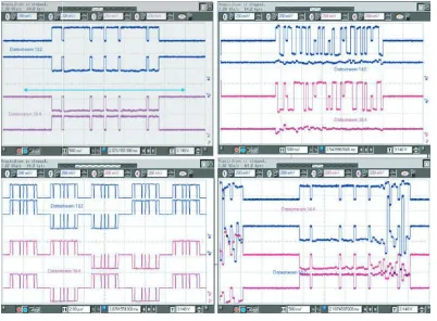
through-Figure 12: Reconstructed pilots and data streams after a 2×3 MIMO-OFDM transmission and real-time spatial separation. Top left: reconstructed OFDM pilot symbol with 48 active subcarriers. Top right: reconstructed two data streams in one OFDM symbol vector using BPSK. Bottom left: reconstructed OFDM pilot sym-bols. Bottom right: reconstructed OFDM pilot symbol affected by fading in the upper frequency band.
put at the highest possible SNR point. We see that the fit-ted curve is steepest for the SVD-MIMO and has the longest tail at low rates for the linear MMSE. This is in good accor-dance with capacity simulations from the measured chan-nels. Especially at low outage probabilities the three schemes have a huge difference in throughput. Example: Outage = 0.01 MMSE: 11 bps/Hz, MMSE-SIC: 17 bps/Hz, and SVD-MIMO: 21 bps/Hz. Those results are comparable with spec-tral efficiencies achieved by [23].
5.3. MIMO-OFDM for frequency-selective channels
The extension of the well-studied flat-fading algorithms to-wards frequency-selective channels offers equalization of the MIMO channel in the time or frequency domain. For reasons of simplicity, a frequency-domain equalization with OFDM was implemented for a 2×3 MIMO system as a first step. 48 out of 64 subcarriers were used for data transmission, com-pliant with 802.11g plus an additional C-preamble for the es-timation of the MIMO channel, which was described in [57]. For a 20 MHz bandwidth version, the OFDM parameters were the following: center frequency: 5.2 GHz, frame length: 2 milliseconds, symbol length: 4 microseconds, guard inter-val: 800 nanoseconds, training sequence length: 64 OFDM symbols maximum.
In order to use as many modules from the flat-fading FPGA design, all correlation units and the multiplication unit (MIMO detector) have to be reused 48× within one OFDM symbol length. Since the signals for each frequency leave the FFT unit one after the other, the filter weights, and so forth, can be changed from subcarrier to subcarrier.
Tx1, I-signal of Tx2, and Q-signal of Tx2. The arrow in the top-left figure shows the symbol length of 4 microseconds. The Hadamard sequences used for the C-preamble are clearly to be seen in the bottom-left figure. In the top-right we see a data symbol vector using BPSK. The degrading effect of sever I/Q imbalance is visible in the remaining image crosstalk in the I/Q-branches which should be zeroed with perfect spatial reconstruction. In the bottom-right figure, we see the noise enhancement after the MMSE MIMO detector due to singu-larities in the MIMO matrices in the upper OFDM frequency band. Here, we do not have to find deep fading as known from SISO systems but instead the MIMO matrix becomes close to singular which causes severe noise enhancement due to the matrix inversion involved with the MMSE filter. This effect degrades all spatial MIMO channels, in general.This observation is very important for proper space-frequency coding since redundant information can be placed at another Tx antenna but must be placed well separated in frequency domain, to avoid degradation from the same “fading hole.”
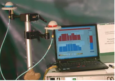
A recent implementation of the MIMO-OFDM with a 100 MHz FPGA design-allowed a 1 Gbps with 3 Tx and 5 Rx antennas and 64 QAM on 48 active subcarriers [64]. An up-grade to 128 subcarriers and channel adaptive bit loading now allows a 1 Gbps transmission with only 2 Tx and 4 Rx antennas when 116 subcarriers are used for data transmis-sion. A revised RF front end allowed 256-QAM in good chan-nels. A first public presentation was given at the CeBIT fair in Hannover in early March.Figure 13shows the bit allocation for a particular channel realization in our lab.
Figure 14shows screen shots of the reconstructed sym-bols at different subcarriers, showing that even with a good image suppression timing imperfections can cause signifi-cant differences in noise enhancement in the real and imagi-nary parts of the data symbol. Therefore, independent mod-ulation in I and Q is an appropriate solution.
6. CONCLUSIONS AND CHALLENGES FOR FUTURE MIMO IMPLEMENTATIONS AND APPLICATIONS
A multiantenna experimental test-bed was presented based on a hybrid approach consisting of FPGAs and DSPs which was developed at FhG-HHI. The internal signal processing structures were described in detail and critical implementa-tion issues were pointed out. The MIMO filter algorithms which were calculated on a DSP were analyzed with regard to complexity and optimization potential in C-code or as-sembly code. Several implementations were compared on the DSP target used for the test-bed and a selection of those algorithms was applied for real-time high data rate MIMO transmission experiments using a single carrier MIMO de-sign and a MIMO-OFDM dede-sign. The experimental results clearly show that multiantenna techniques are an essential ingredient of signal processing structures for future wireless systems. The spatial diversity and multiplexing gains could be measured in good accordance with what was predicted from information theory. Using channel adaptive bit load-ing in the sload-ingle-carrier mode, average spectral efficiencies of more than 20 bps/Hz with an assured BER better than 10−2
Figure 13: Demonstration of MIMO-OFDM with adaptive bit loading at CeBIT 2005 in Hannover, Germany. 2 Tx and 4 Rx anten-nas, 5.2 GHz, 100 MHz bandwidth, and 116 active OFDM subcar-riers out of 128. The bit allocation per antenna and per subcarrier can be seen on the screen.
could be achieved. The maximum possible rates with the flat fading 4×5 MIMO design was 160 Mbps using 5 Msymbol vectors per second and 256-QAM while a 3 ×5 MIMO-OFDM design could carry a peak rate of 1 Gbps when using 64-QAM. These initial experimental results show that MIMO techniques are feasible with state-of-the-art signal processing capabilities and can be used to enhance the performance of wireless communication systems significantly.
Recent implementation of MIMO-OFDM with 100 MHz bandwidth has showed that the flat-fading MIMO algo-rithms for the DSP and many VHDL components could be reused with only slight changes for the MIMO-OFDM signal processing.
Necessary further steps towards higher spectral efficiency and possible transmission rates of beyond 1 Gbps are out-lined in the following together with some of the technical challenges involved.
If a higher bandwidth efficiency with OFDM is desired the number of subcarriers should be increased since the length of the guard interval is generally determined by the deployment scenario. Therefore, faster MIMO-filter compu-tation is required, which could be solved by parallel comput-ing, filter interpolation, faster clocking of the DSPs, and as-sembly code.