Controlling nonlinear infinite dimensional systems via the initial state

warwick.ac.uk/lib-publications

Original citation:

Evans, Neil D. (2013) Controlling nonlinear infinite-dimensional systems via the initial state.

SIAM Journal on Control and Optimization, 51 (5). pp. 3757-3780.

Permanent WRAP URL:

http://wrap.warwick.ac.uk/97922

Copyright and reuse:

The Warwick Research Archive Portal (WRAP) makes this work by researchers of the

University of Warwick available open access under the following conditions. Copyright ©

and all moral rights to the version of the paper presented here belong to the individual

author(s) and/or other copyright owners. To the extent reasonable and practicable the

material made available in WRAP has been checked for eligibility before being made

available.

Copies of full items can be used for personal research or study, educational, or not-for-profit

purposes without prior permission or charge. Provided that the authors, title and full

bibliographic details are credited, a hyperlink and/or URL is given for the original metadata

page and the content is not changed in any way.

Publisher’s statement:

Published in SIAM Journal on Control and Optimization 2013.

A note on versions:

The version presented here may differ from the published version or, version of record, if

you wish to cite this item you are advised to consult the publisher’s version. Please see the

‘permanent WRAP URL’ above for details on accessing the published version and note that

access may require a subscription.

VIA THE INITIAL STATE

NEIL D. EVANS∗

Abstract. A control problem is considered for nonlinear time-varying systems described by partial differential equations, in which the control acts only via part of the initial state. The problem is to drive part, or all, of the process to some desired state in a specified time. The motivation for such systems are control problems arising in medicine and biology that involve spatial or age characteristics, or time-delays. The approach taken is to formulate the problem as a fixed point problem for a suitable abstract differential equation and then apply a version of the Contraction Mapping Theorem. Conditions are imposed so that the problem is well defined and a weaker form of solution exists. The solution obtained ensures that the target state is achieved on the range of a linear operator arising from a linearisation of the system about an initial estimate for the control. Although the Contraction Mapping Theorem yields a constructive method to determine the solution an alternative, more direct, approach is presented, which relies on an iterative scheme for the control and the original dynamics.

Key words. distributed parameter systems, initial state control, fixed point theorems

AMS subject classifications. 93C10, 93C20, 93C25

1. Introduction. The control problem which this paper considers is to drive some part (or all) of a particular process to some desired state in a specified time, when the control acts only via the initial state. For example, in [7] the problem of controlling the spread of rabies in a fox population was considered where the initial distribution of vaccinated and/or culled foxes had to be chosen such that the combined distribution of infected foxes was some desired target. In this case the parts of the system that were controlled were the population densities of incubating and rabid foxes, while the control represented the distribution of vaccinated and/or culled foxes produced via a suitable intervention. In [7] the control problem was formulated in terms of an abstract differential equation with the part of the state to be controlled as an output. Thus the problem became that of driving the output of the system to a desired value in a specified time using only an input term in the initial condition.

This paper addresses the problem in [7] in a more general setting that permits unboundedness of the nonlinearity and proposes an alternative, iterative scheme for determining the required control. In addition, the control problem is generalised slightly by permitting multiple impulsive inputs. The mathematical formulation of the control problem is as follows: Consider the system of differential equations on a Banach spaceZ given by the following

˙

zi(t) =f(t, zi(t)), zi(τi) =zi₋1(τi) +Bui, i= 1, . . . , m,

where f is nonlinear, them inputs,u1, . . . ,um, are applied at times 0 =τ1< τ2 <

· · · < τm, and z0(0) = z0 denotes the known, given initial state of the equation without input. The linear operatorB determines how the control acts via the given state. he states from these systems of equations can be pieced together to form the trajectoryz(t) =zi(t), fort∈[τi, τi+1),i= 1, . . . , m, whereτm+1=T for some fixed timeT.

The controls, ui, are assumed to belong to the same Hilbert space U such that

B _{∈ L}(U, Z). Therefore the treatment of this paper is confined to the situation

∗_{School of Engineering, University of Warwick, Coventry CV4 7AL UK}

(Neil.Evans@warwick.ac.uk_).

involving bounded inputs. If, for the underlying system, it is not possible to affect the state at every point of the spatial domain so that the controls are restricted to only a few points or parts of the boundary the resulting model will involve an unbounded input operator. Following the approach of [16] for systems with unbounded inputs and outputs, it can be assumed that there exists a Banach spaceZ_⊂Z1 with continuous injection and dense range. The input operator is then assumed to be bounded from

U toZ1.

The output associated with the differential equation is given by

y=Czm(T),

whereT is the specified time and the output takes values in a Hilbert spaceY. The control problem is to choose the ui such that the resulting output is y = yd, the desired target output.

Suppose that initial guesses are made for the control, ˆui say, with associated differential equations

˙ˆ

zi(t) =f(t,zˆi(t)), zˆi(τi) = ˆzi₋1(τi) +Bu,ˆ (1.1)

where ˆz0(0) =z0 and that these equations have continuously differentiable solutions ˆ

zi(·). While this control might be a good initial guess there is no reason to assume that the output of this system, Czˆm(T), is the desired final state. Therefore a local approximation is made by settingzi= ˆzi+zi andui= ˆui+ui to get

˙

zi(t) + ˙ˆzi(t) =f(t, zi(t) + ˆzi(t)), zi(τi) =zi−1(τi) +Bui, (1.2)

for i= 1, . . . , m, where z0(0) = 0. Now suppose that f is differentiable around the trajectory_{(t, z′_{(t)) :t∈[0, T]} in the sense that}

f(t, zi) =f(t,zˆi(t)) +A(t) (zi−zˆi(t)) +N(t,(zi−zˆ(t))) (1.3)

for some piecewise continuousA(·) such thatA(t) is an unbounded linear operator on

Z for eacht ∈[0, T]. In the following, to permit unboundedness of the nonlinearity on Z, it will be assumed that there are Banach spaces Z and Z such that that

N : [0, T]×Z −→ Z. More precise assumptions will be introduced in the following section.

Equation (1.2) therefore can be rewritten as

˙

zi(t) =A(t)zi(t) +N(t, zi(t)), zi(τi) =zi₋1(τi) +Bui, (1.4)

fori= 1, . . . , m, wherez0(0) = 0.

In_§3 the first stage of the control problem is considered, namely the construction of inputs that give rise to a mild solution with the desired properties. A fixed point theorem is applied to give the solution using the following version of the Contraction Mapping Theorem from [2]:

Theorem 1. Suppose that ϕ: W −→W is a mapping between Banach spaces that satisfies

kϕx₋ϕy_{k ≤}k_kx₋y_k, 0_≤k <1

(k a constant), forx, y_∈D, a subset of W. If both the ball

S=

w∈W :kw−w1k ≤ k

1−kkw1−w0k

and w0 lie in D, then the iterative process wi+1 =ϕwi converges to a unique fixed-point inD.

The earliest use of fixed point methods in a control context was in [8] for finite-dimensional systems. In [4] the application of fixed point methods to finite-finite-dimensional time-varying systems was presented, and this approach has been extended to infinite-dimensional systems in [11]. An early review of the use of fixed point methods in nonlinear control and observation is provided in [1].

In§2 the general framework for considering the control problem is proposed and the control problem itself is solved in§3 using a fixed point approach. An equivalent, but less intuitive, method for constructing the control is given in §4. This method exploits the original system dynamics and uses an adaptive scheme to give the so-lution. This method readily lends itself to numerical simulation and constructs the control directly rather than via a mild solution (as is the case in the fixed point ap-proach). Motivated by the example in [7] a class of systems is considered in _§5 in which the linear part of the dynamics arises from a time-varying perturbation of the (time-invariant) generator of a strongly continuous semigroup. In contrast with [7] the perturbation is permitted to exhibit unboundedness comparable with that of the nonlinearity. Finally to illustrate the application of the approach proposed in this paper a case study is considered in_§6, in which the problem of determining a dosing schedule to control the viral load in a HIV patient is solved. The solution exploits the iterative approach of _§4 applied to the numerical solution of the system delay-differential equations. This case study illustrates how even the single input version (m = 1) of the theory can be applied to yield results for multiple inputs. For the case study this is achieved because the inputs affect states that appear linearly in the model so that the system can be formulated in terms of a delay differential system.

2. Mathematical framework. In this section the general system given by

˙

zi(t) =A(t)zi(t) +N(t, zi(t)), zi(τi) =zi−1(τi) +Bui, (2.1)

is considered in order to provide an abstract framework in which to tackle the control problem. Consider for the moment the linear part of (2.1), with arbitrary initial state, given by

˙

zi(t) =A(t)zi(t), zi(s) =zs, (2.2)

withs_∈[0, T]. In the time-invariant case, ifAis a densely defined linear operator on

Z with non-empty resolvent setρ(A), then it is well known that the Cauchy problem (2.2) is well-posed if and only ifAis the generator of a strongly continuous semigroup [15]. In the time-varying case the situation whereA(t) is the generator of a strongly continuous semigroup for each t _∈[0, T] was considered in [17] and that whenA(t) is strongly continuous with domain independent oft in [10]. Adopting the setting in [9], who weakened the latter assumption, the following assumption is made:

Assumption 1. A(t) is a linear operator on Z for all t ∈ [0, T] with domain

D(A), which is independent oftand dense inZ. For allz∈D(A)the mapt7→A(t)z

is continuous except on a finite set of discrete pointsJ. For eachτ∈J andz∈D(A) the one-sided limitslimt_↓τA(t)z,limt_↑τA(t)z exist.

For the full problem (2.1), even in the time-invariant case with bounded non-linearity, in general it cannot be guaranteed that the resulting Cauchy problem is well-posed. However, if N(_·, z(_·)) _∈ P C(s, T;Z) and the Cauchy problem is well-posed with solutionz(_·), and strong evolution operatorU(t, s), then

z(t) =U(t, s)zs+

Z t

s

U(t, σ)N(σ, z(σ)) dσ.

Therefore, in the following, the control problem will first be considered with respect to the corresponding mild solutions:

zi(t) =U(t, τi) (zi−1(τi) +Bui) +

Z t

τi

U(t, s)N(s, zi(s)) ds, (2.3)

fori= 1, . . . , m, where z0(0) = 0 andui∈U, a Hilbert space such thatB∈ L(U, Z) andU(t, s) is a mild evolution operator onZ. Suppose that the following assumptions hold:

TV 1. Z_⊂Z are Banach spaces such that the nonlinearityN : [0, T]_×Z_−→Z

maps functions in Lp_{(0, T;Z)to functions in L}q_{(0, T;Z)for real numbers p, q}

≥1 in the sense that

(_Nz) (_·) =N(_·, z(_·))_∈Lq_{(0, T;Z) whenever z(}

·)_∈Lp_{(0, T;Z).}

TV 2. U(t, s)is a mild evolution operator on all three spacesZ,Z andZ.

TV 3. There exists a k1(·) ∈ Lr_{(0, T), with} 1 r+

1 q =

1

p + 1, such that for all (t, s)_∈∆(T),U(t, s)_{∈ L}(Z, Z)and

kU(t, s)z_kZ ≤k1(t−s)kzkZ for allz∈Z. (2.4)

Let K1=kk1(·)kLr(0,T).

TV 4. There exists ak2(_·)_∈Lp_{(0, T)such that for all(t, s)}

∈∆(T)andu_∈U,

U(t, s)Bu_∈Z and

kU(t, s)BukZ ≤k2(t−s)kukU. (2.5)

Let K2=kk2(·)kLp_(0,T).

The above assumptions ensure that the following operator is well-defined (inZ)

(M_{Uh) (t) =}

Z t

0

U(t, s)h(s) ds for allh(_·)_∈Lq_{(0, T;Z). (2.6)}

Moreover, the mapt_7→(M_{Uh) (t) is continuous with respect tok·kZand the following}

notion of weak solution is well defined for (2.3):

Definition 1. A mild solution of (2.3) is any piecewise-continuous function

z(·)∈P C(0, T;Z) (with discontinuities at t =τi) such that z(t)∈Z for almost all

t ∈[0, T], z(·) isLp-integrable in Z on every interval[0, t] and (2.3) is satisfied for allt_∈[0, T].

Therefore a mild solution,z(·), of (2.3) is sought such that the output given by

wherey _∈Y for a suitable Hilbert spaceY, is some specified valueyd. For consider-ations to be discussed in greater detail later, it is necessary to assume that the range ofφis a closed subspace ofY, and therefore it might not be possible to considerCas a bounded linear operator fromZ toY. Therefore, the following assumption is made:

TV 5. There exists a Banach spaceV _⊂Z, with continuous injection, such that

C _{∈ L}(V, Y). In addition, for all k = 1, . . . , m and u_∈ U, U(T, τk)Bu ∈ V, with constant K3 such that

kU(T, τk)Bu_kV ≤K3kukU.

There exists a constantK4 such that (MUh) (T)∈V and

k(M_{Uh) (T)kV ≤K4khk}

Lq_(0,T;Z)

for allh_∈Lq_{(0, T;Z).}

3. The control problem. Considering for the moment only the linear dynam-ics, the control problem is to find ˜ui (i= 1, . . . , m) such that the output

y=Cˆz(T) +CU(T, τm) (Bu˜m+zm₋1(τm))

=Cˆz(T) + m

X

k=1

φku˜k whereφk =CU(T, τk)B,

is the desired value yd. For the Hilbert space_U =Um _{with inner product}

hu, v_iU =

Pm

k=1huk, vkiU, let Φ : U −→ Y be the linear map defined by Φ(˜u1, . . . ,u˜m) =

Pm

k=1φku˜k. If yd −Czˆ(T) ∈ ran Φ then a solution exists. In particular, if Φ is invertible, then there is a unique solution given by

˜

u= (˜u1, . . . ,u˜m) = Φ−1(yd−Czˆ(T)).

Therefore the linear part of the system can be steered to{y∈Y :y−Czˆ(T)∈ran Φ}. In the literature [12, 1] it is usual to consider the nonlinear problem on this subspace, with some suitable topology defined on it:

Lemma 1. The range ofΦis a Banach spaceR(Φ), with a suitably defined norm. Proof. Since Φ is a bounded linear operator, define the spaceX by

X :=U/ker Φ.

Since ker Φ is closedX is a Banach space under the norm

k[u]_kX= inf

u_∈[u]kukU= infΦ˜u=0 ku+ ˜ukU.

Now define ˜Φ :X −→Y by

˜

Φ[u] = Φ˜u u˜_∈[u].

Then ˜Φ is injective and

kΦ[˜ u]kY ≤ kΦk k[u]kX.

Now define a norm on the range of ˜Φ by

This norm is equivalent to the graph norm on D( ˜Φ−1_{). Since ˜Φ is bounded and}

D( ˜Φ)(= X) is closed it holds that ˜Φ is a closed linear operator and so ˜Φ−1 _{is also} closed [18]. Therefore it follows thatR(Φ) is a Banach space with the above norm.

For anyyd∈Y such thatyd−Czˆ(T)∈R(Φ), sinceU is a Hilbert space and ker Φ is closed the infimum in the definition of_{k · k}X is attained and so there is a u∈ U such that u= ˜Φ−1_(y

d−Czˆ(T)) that minimiseskukU over all controls that achieve

y = yd. Thus a more general form of the linear problem is to find a least squares solution that minimises

k[yd−Czˆ(T)]−ΦukY (3.1)

over all choices of u_{∈ U}, and with the smallest norm in _U. This control, provided

yd−Czˆ(T)∈ran Φ + (ran Φ)⊥, is given by [14]

˜

u= Φ†_(y

d−Czˆ(T)) where Φ†_{is the generalised inverse of Φ.}

For the nonlinear problem this suggests that the control given by

˜

u= Φ† _y

d−Czˆ(T)−C

Z T

0

U(T, s)N(s, z(s)) ds

!

(3.2)

be applied. However this is an implicit expression since the statez(_·) is dependent on the control. If a solution exists then the output is driven to the following

y= ΦΦ†yd+ I−ΦΦ†

"

Czˆ(T) +C

Z T

0

U(T, s)N(s, z(s)) ds

#

. (3.3)

If Φ is invertible then Φ† _{= Φ}−1 _{and (3.3) reduces to y =yd. If Φ is not invertible,} butyd−Czˆ(T)∈ran Φ, then (3.3) reduces to the following:

y=yd+ I−ΦΦ†

"

C

Z T

0

U(T, s)N(s, z(s)) ds

#

.

Remark 1. The first term of(3.3), in the case where the range ofΦis closed, is the orthogonal projection ofyd ontoran Φand the second is the orthogonal projection ontoran Φ⊥_{. Therefore, on the range ofΦ, the control drives the system to the desired} final state.

For notational convenience denote by ˜U(t, s) the family of bounded linear opera-tors defined as follows:

˜

U(t, s)z=

(

U(t, s)z t_≥s

0 t < s

forz_∈Z. Therefore the controllability problem is reduced to that of finding a fixed point of the following map,ψ:Lp_{(0, T;Z)}

−→Lp_{(0, T;Z):}

(ψz)(t) = m

X

k=1 ˜

U(t, τk)Bu˜k+ (MUNz) (t), (3.4)

where ˜u= Φ†_{(yd−Czˆ(T)−C(}M_{UNz) (T)). Once a fixed point has been found this}

following result from [14] is important for the main theorem of this paper because it characterises when the generalised inverse of a bounded linear operator is itself bounded.

Lemma 2. Let Φ : U _−→ Y be a bounded linear operator between two Hilbert spaces. Then the generalised inverseΦ† _{is bounded if and only if the range ofΦ is a} closed subspace ofY.

Theorem 2. Consider the nonlinear system governed by

z(t) = m

X

k=1 ˜

U(t, τk)Buk+

Z t

0

U(t, s)N(s, z(s)) ds, (3.5)

whereU(t, s)is a mild evolution operator onZ, with output given by

y=Cz(T) +Cˆz(T) (3.6)

for a given outputCzˆ(T). Suppose that the following conditions are satisfied: 1. Assumptions TV 1–5 hold.

2. The range of φis a closed subspace ofY.

3. The nonlinearity _N satisfies the following Lipschitz condition on the ball of radiusa′ _{about the origin, Ba}′:

kNz− NwkLq_(0,T;Z)≤k(kzk,kwk)kz−wkLp_(0,T;Z) (3.7)

for each z, w _∈ Ba′ and some continuous symmetric function k(·,·) :R+×

R+_−→R+ _{such that k(0,0) = 0.}

4. Choosea≤a′ _{such that}

√_{m K}

2kΦ†k kCkK4+K1K˜ =K <1 (3.8)

whereK˜ = sup0≤θ1,θ2≤ak(θ1, θ2). Suppose thatyd∈Y satisfies

kyd−Czˆ(T)kY ≤

a(1₋K)

√_{m K}

2kֆk

. (3.9)

Then there exists a control ˜uof the form (3.2) that drives the output (3.6) toyd on the range ofΦ.

Proof. The first step of the proof is to show thatψ is a contraction onBa:

kψz₋ψw_kLp_(0,T;Z)≤√m K₂kΦ†C(M_U(Nw− Nz)) (T)k_U

+k(M_{U(Nz− Nw)) (·)kL}p_(0,T;Z)

≤ √m K2kΦ†k kCkK4+K1K˜kz−wkLp_(0,T;Z).

Therefore by (3.8)ψis a contraction onBa.

Since the initial guess for the control has been included in the initial state for ˆz, it seems natural to consider the iterative process given by zn =ψzn₋1 withz0 = 0. Then it is seen that

z1(t) = m

X

k=1 ˜

LetS =nz∈Lp(0, T;Z) :kz−z1kLp_(0,T;Z)≤ K

1₋Kkz1kLp_(0,T;Z)

o

. This will be con-tained in the ball of radiusaif

1 + K 1−K

k

m

X

k=1 ˜

U(·, τk)BukkLp_(0,T;Z)≤a,

which will be the case if

1 1−K

√

m K2kΦ†k kyd−Czˆ(T)kY ≤a.

Rearranging this inequality yields (3.9) and so applying Theorem 1 proves the exis-tence of a unique fixed point forψ. Substituting this fixed point into (3.2) gives the control ˜u.

Note that the output resulting from applying the control given by the last theorem is only guaranteed to coincide with the desired state on the range ofφ. If there exists a control ˜usuch that the output, when applying this control, is the desired state, then it remains an open question whether the previous theorem gives the same control.

The proof of Theorem 2 provides an iterative scheme for obtaining the fixed point (and hence the control). In the next section a more direct method of finding the required control (and hence the fixed point) is given.

4. Iterative method for constructing control. The constructive method of the proof of Theorem 2 can be used to find the control that solves the control problem, but the desired control is found indirectly from the fixed point solution. In this section an alternative method for obtaining the control that gives rise to the solution of the fixed point problem is constructed. The method exploits the original dynamics and directly determines the required control without the need for further substitution.

The method used in this section is as follows: Consider the dynamical equations

zn(t) = m

X

k=1 ˜

U(t, τk)Bu(n)k+ (M_{UNzn) (t) (4.1)}

where (as before)U(t, s) is a mild evolution operator on Z and the output is given by the following

yn=Czn(T) +Czˆ(T). (4.2)

The controlu(n+ 1) is defined in terms of the previous control as follows

u(n+ 1) =u(n) + Φ†_(y

d−yn).

For eachn∈N_{it must be shown that there exists a solution of the dynamical equation}

and that the iterative scheme foru(n) converges to the required solution of the fixed point problem.

Theorem 3. For each n_∈N_{consider the nonlinear system governed by}

zn(t) = m

X

k=1 ˜

U(t, τk)Bu(n)k+ (MUNzn) (t). (4.3)

2. The range of φis a closed subspace ofY.

3. The nonlinearity _N satisfies the following Lipschitz condition on the ball of radiusa′ _{about the origin, Ba}′:

kNz_{− N}w_kLq_(0,T;Z)≤k(kzk,kwk)kz−wkLp_(0,T;Z) (4.4)

for each z, w _∈ Ba′ and some continuous symmetric function k(·,·) :R+×

R+_−→R+ _{such that k(0,0) = 0.}

4. Choosea_≤a′ _{such that}

√_{m K}

2kΦ†k kCkK4+K1K˜ =K <1 (4.5) whereK˜ = sup0_≤θ₁,θ_2≤ak(θ1, θ2).

Suppose thatyd∈Y satisfies

kyd−Czˆ(T)kY ≤

a(1₋K)

√

m K2kֆk

. (4.6)

Then the iterative schemeu(0) = 0,

u(n) =u(n−1) + Φ†(yd−yn₋1) n≥1,

gives rise to a mild solutionzn of(4.3)for eachnand the sequence of controls,u(n), converges to the fixed point solution, u˜, of Theorem 2.

Proof. The theorem is proved in two steps: Firstly it is shown inductively that the scheme gives rise to a solutionzn for eachn∈N. Then it is shown that the scheme converges and that the limit is the fixed point solution from the previous section.

To show the existence of each solution,zn, of (4.3) Theorem 1 will be applied to the operator Ψ :Lp(0, T;Z)−→Lp(0, T;Z) given by

(Ψzn) (t) = m

X

k=1 ˜

U(t, τk)Bu(n)k+ (MUNzn) (t). (4.7)

Suppose thatu(n)_{∈ U} satisfies

ku(n)kU≤

a1₋K1K˜

√_{m K}

2 . (4.8)

Ψ is a contraction on the ballBa since, forz, w∈Lp(0, T;Z)

kΨz−ΨwkLp_(0,T;Z)=k(MUNz) (·)−(MUNw) (·)kLp_(0,T;Z)

≤K1K˜kz−wkLp_(0,T;Z).

Therefore by (4.5) Ψ is a contraction.

For the iterative schemewn+1= Ψwn, starting withw0= 0, it is seen that

w1(t) = m

X

k=1 ˜

U(t, τk)Bu(n)k

and so let S =

(

w:kw−w1kLp_(0,T;Z)≤

K1K˜ 1−K1K˜k

w1kLp_(0,T;Z)

)

. S will be

con-tained inBa if

1 + K1K˜ 1₋K1K˜

!

k

m

X

k=1 ˜

which will certainly be the case if

1 1−K1K˜

√

m K2kunkU ≤a

that is, if (4.8) is satisfied, and so applying Theorem 1 ensures the existence of a unique fixed pointzn of Ψ.

Trivially, sinceu(0) = 0 the inequality (4.8) is satisfied forn= 0 giving a solution

z0= 0. Now inductively, if solutions,zk(t), of (4.3) exist fork < n, then

u(n) = 1−Φ†Φ

u(n−1) + Φ†(yd−Czˆ(T)−C(MUNzn₋1) (T)) =. . .= Φ†(yd−Czˆ(T)−C(MUNzn₋1) (T))

and so

ku(n)kU≤ kΦ†k(kyd−Czˆ(T)kY +kC(MUNzn₋1) (T)kY)

≤ kΦ†k

 

a1₋K+√mKK˜ 2kΦ†k kCkK4

√_{m K}

2kBk kֆk

 =

a1₋K1K˜

√_{m K}

2

.

Therefore, for eachn∈N_{there exists a solution zn of (4.1).}

Now it is shown that the iterative scheme foru(n) converges: Observe that

ku(m)−u(n)kU =kΦ†C(MU(Nzn₋1− Nzm₋1)) (T)k_U

≤ kΦ†_{k kCkK}

4K˜ kzm−1−zn−1kLp_(0,T;Z)

and so

kzm−znkLp_(0,T;Z)=k

m

X

k=1 ˜

U(_·, τk)B(u(m)k₋u(n)k) + (M_{U(Nzm− Nzn)) (·)kL}p

≤ √

m K2kΦ†k kCkK4K˜ 1−K1K˜ k

zm₋1−zn₋1kLp_(0,T;Z).

Therefore, by (4.5) the sequence of solutions,zn, (and hence controlsu(n)) converges asn_{→ ∞}. Now

u(n) = Φ†_(y

d−Czˆ(T)−C(MUNzn−1) (T))

and so lettingn_{→ ∞}, since Φ† _andC(M_{U·) (T) are bounded, the limit is given by}

u= Φ†_(y

d−Czˆ(T)−C(MUNz) (T)), but thenz (the limit of the sequence (zn)_n∈N) satisfies

z(t) = m

X

k=1 ˜

U(t, τk)Buk+ (MUNz) (t), u= Φ†(yd−Czˆ(T)−C(MUNz) (T))

and so is a fixed point ofψ. Hence the iterative and fixed point schemes converge to the samez and yield the same control.

Consider the single input case and suppose that (as considered in [7]) the original dynamics are semilinear in form:

˙

where A is the generator of a strongly continuous semigroup, S(t), on Z and g : [0, T]_×Z _−→ Z is strictly nonlinear and continuously differentiable. If an initial guess, ˆu, is made for the control such that z0 +Buˆ ∈ D(A), then there exists a classical solution, ˆz(_·), of the initial value problem on [0, T] [15]. IfP(t) = dg(ˆz(t)), the derivative of g with respect to z evaluated at ˆz(t), then P(_·) _∈ C(0, T;_L(Z)). Define the following function from [0, T]_×Z _−→Z:

N(t, z) =g(t, z+ ˆz(t))−g(t,zˆ(t))−P(t)z.

Therefore, settingz= ˆz+z andu= ˆu+ugives

˙

z(t) = (A+P(t))z(t) +N(t, z(t)), z(0) =Bu,

which is of the form (2.1) withZ =Z =Z andA(t) =A+P(t). The assumptions above ensure thatA(_·) =A+P(_·) is the generator of a mild evolution operator,U(t, s), onZ that is uniformly bounded [3] (in fact U(t, s) is a weak evolution operator [9]). Therefore it is seen that assumptions TV 1–4 are satisfied.

Sincegis continuously differentiable it satisfies a local Lipschitz condition in that there exists a constantk_∗(c) such that

kg(t, z1)₋g(t, z2)_kZ ≤k∗(c)kz1−z2kZ

for zi ∈Z with kzikZ ≤ c. Therefore, the nonlinear operator N(·,·) is also locally Lipschitz since, forzi ∈Z withkzikZ ≤c,

kN(t, z1)₋N(t, z2)_kZ ≤ kg(t, z1+z′(t))−g(t, z2+z′(t))kZ+kP(t) (z1−z2)kZ

≤ k_∗(c+η) + sup

t_∈[0,T]k

P(t)kL(Z)

!

kz1−z2kZ

whereη=kz′_{(·)kC(0,T;Z).}

A further control u is then sought such that, if z(_·) is a solution of (4.9) with initial state

z(0) =z0+Buˆ+Bu,

then

Cz(T) =yd

for some fixedT andyd. Now consider a sequence of controls (un)n_∈Nthat are related via the iterative scheme so that thenth _control,u

n is given by

un=un₋1+ Φ†(yd−yn₋1),

and suppose that the differential equation (4.9) can be solved for the corresponding sequence of initial states

zn(0) =z0+Buˆ+Bun₋1+BΦ†(yd−yn₋1)

5. A class of perturbed systems. Motivated by the final remarks of the pre-vious section consider systems in which the linear operator A(_·) is obtained by an unbounded perturbation of some time invariantA:

˙

zi(t) = (A+P(t))zi(t) +N(t, zi(t)), zi(τi) =zi−1(τi) +Bui, (5.1)

where z0(0) = 0. For simplicity the degree of unboundedness of the perturbation is the same as that of the nonlinearity, and so P(·) ∈P C(0, T;L(Z, Z)). Based on the Pritchard-Salamon class of systems introduced in [16] to study linear quadratic optimal control for infinite-dimensional systems with unbounded input and output operators, suppose that the following assumptions hold for (5.1):

PS 1. Z⊂Z ⊂Z are Banach spaces such that the canonical injections Z ֒→Z,

Z ֒_→ Z are continuous with dense ranges. Moreover, the nonlinearity N : [0, T]_×

Z _−→Z maps functions in Lp_{(0, T;Z) to functions in L}q_{(0, T;Z) for real numbers}

p_≥q_≥1 in the sense that_Nz _∈Lq_{(0, T;Z) wheneverz}

∈Lp_{(0, T;Z). In addition,}

P(_·)_∈P C(0, T;_L(Z, Z)).

PS 2. A is the generator of a strongly continuous semigroup, S(t), onZ, which is also a strongly continuous semigroup onZ andZ.

PS 3. There exists a continuous ka(_·) : [0, T] _−→ R+_{, and for all s ∈ [0, T),} h(_·)_∈L2_{(s, T;Z), the mapt}

7→Rt

sS(t−σ)h(σ)dσis continuous from[s, T] toZ and

Z t

s

S(t₋σ)h(σ)dσ

_Z≤

ka(t₋s)_kh(_·)_kL2(s,t;Z). (5.2)

PS 4. There exists aKb>0 such that

kS(·)zkL2(0,T;Z)≤KbkzkZ (5.3)

for everyz_∈Z.

In addition, the following assumption is sufficient to provide the necessary smooth-ing properties with respect to the possible unboundedness of the output operatorC:

PS 5. There exists a Banach space V _⊂Z, with continuous injection, such that

C_{∈ L}(V, Y). In addition, there exist a continuouskc : [0, T]−→R+ and a constant

Kd such that for all s∈[0, T)andh(·)∈L2(s, T;Z),

RT

s S(T −σ)h(σ)dσ∈V,

Z T

s

S(T−σ)h(σ)dσ

V

≤kc(s)kh(·)kL2(s,T;Z) (5.4)

and for allk= 1, . . . , m andu∈U,S(T−τk)Bu∈V,

kS(T−τk)BukV ≤KdkukU.

Theorem 4. Suppose that conditions PS 1–3 are satisfied. ThenA(·) =A+P(·) is the generator of a mild evolution operatorU(t, s)onZ in the sense that U(t, s)is the unique, in the class of strongly continuous operators on Z, solution of

U(t, s)z=S(t₋s)z+

Z t

s

S(t₋σ)P(σ)U(σ, s)zdσ (5.5)

Proof. Fixs_∈[0, T] and define an operator Γs:P_∞(s, T;_L(Z))_−→P_∞(s, T;_L(Z)) by

Γs(U)(t)z:=S(t₋s)z+

Z t

s

S(t₋σ)P(σ)U(σ)zdσ. (5.6)

Note that

kΓs(U1)(t)₋Γs(U2)(t)_kL(Z)≤γ(t−s)1/2kPk kU1(·)−U2(·)kP∞

whereKa= sups≤t≤Tka(t−s) and so by induction

kΓks(U1)−Γks(U2)kP∞ ≤

_(T

−s)k

k!

1/2

(KakPk)kkU1(·)−U2(·)kP∞.

By choosingksuch thath(T−_k!s)ki1/2(KakPk)k <1 it is seen that Γsis a contraction onP_∞(s, T;_L(Z)). Therefore there exists a unique fixed pointU(_·, s) of (5.6). This fixed point is given byU(t, s) =P∞

n=0Un(t, s) whereU0(t, s)z=S(t−s)zand

Un(t, s)z=

Z t

s

S(t−σ)P(σ)Un₋1(σ, s)zdσ.

ClearlyU(s, s) =I and note that, forz_∈Z,

kU(t, r)U(r, s)z₋U(t, s)z_kZ

=

Z t

r

S(t−σ)P(σ) (U(σ, r)U(r, s)z−U(σ, s)z) dσ

Z

≤ka(t−s)kPk k(U(·, r)U(r, s)z−U(·, s)z)k_L2_(r,t;Z).

Therefore, settingg(α) =_kU(α+r, r)U(r, s)z₋U(α+r, s)z_k2

Z it follows that

0≤g(t−r)≤

Z t−r

0

[const]g(σ) dσ

and so applying Gromwell’s LemmaU(t, s) =U(t, r)U(r, s). Suppose that sup0_≤t_≤TkS(t)kL(Z)=M0,z∈Z and consider

kUn(t, s)z_kZ ≤KakPk kUn−1(·, s)zkL2(s,t;Z)

≤

_(t

−s)n

n!

1/2

(KakPk)nM0kzkZ.

Therefore the series givingU(t, s) is majorised by

M0 ∞

X

n=0

_(t

−s)n

n!

1/2

(KakPk)n

In fact the smoothing properties of the semigroup, PS 3 and PS 4, are sufficient forU(t, s) to be extended to a mild evolution operator onZ andZ:

Corollary 1. Suppose that the hypotheses of Theorem 4, together with PS 4, are satisfied and let U(t, s) be the corresponding mild evolution operator. Then an extension of U(t, s) to a bounded linear operator onZ can be defined by

˜

U(t, s)z:= lim

n→∞U(t, s)zn

for each z ∈ Z, where (zn)∞_n=1 is a sequence into Z such that kzn −zk_Z → 0 as

n → ∞. Furthermore, this extension, which will be denoted by U(t, s), is a mild evolution operator onZ andZ.

Proof. First note that there exist positive constants,R1andR2, such thatkzkZ ≤

R1kzkZ≤R1R2kzkZ for allz∈Z. Letz∈Z and consider

kUn+1(t, s)zkZ ≤KakPk kUn(·, s)zkL2(s,t;Z)

≤

(t−s)n

n!

1/2

(KakPk)n+1Kbkzk_Z

so that there exists a constant, M1, such that _kU(t, s)z_kZ ≤M1kzkZ for all z ∈Z. Therefore it is seen thatU(_·,_·) is uniformly bounded with respect to_{k · k}Z andk · kZ, with bounds denoted byMU andMU.

Now forz∈Z, let (zn)∞_n=1 be a sequence intoZ such thatkzn−zk_Z →0. Then

kU˜(t, s)zkZ = lim_n

→∞kU(t, s)znkZ≤nlim_→∞MUkznkZ =MUkzkZ

and so the extension of U(t, s) to Z (andZ) is also uniformly bounded. It is clear that ˜U(t, t)z=zfor allz_∈Z, and if (t, s)_∈∆(T), withr_∈[s, t], then

kU(t, r)U(r, s)zn−U˜(t, s)zkZ =kU˜(t, s)zn−U˜(t, s)zkZ≤MUkzn−zkZ −→0

asn→ ∞. Therefore ˜U(t, s)z= ˜U(t, r) ˜U(r, s)z for allz∈Z. To see that ˜U(_·,_·) is strongly continuous note that

kU˜(t, s)z−U(t, s)znk_Z =kU˜(t, s)z−U˜(t, s)znk_Z ≤MUkzn−zk_Z

and so ˜U(·, s)z is the uniform limit of a sequence of continuous functions, U(·, s)zn. Similarly, ˜U(t,·)z is also continuous and the extension ˜U(t, s) is a mild evolution operator onZ andZ, which will be denoted byU(t, s) in the following.

Remark 2. In proving the uniform boundedness of the mild evolution operator in Corollary 1 it is seen that there exists a constantM1 such thatkU(t, s)zkZ≤M1kzkZ for all z _∈Z. Therefore the extension to Z satisfies U(t, s)_{∈ L}(Z, Z) with uniform boundM1. HenceU(t, s)satisfies TV 3. Moreover, _kU(t, s)Bu_kZ ≤R1M1kBk kukU for allu∈U so that TV 4 is also satisfied.

Remark 3. Note that if PS 5 is satisfied then for allz∈Z

Z T

s

S(T−σ)P(σ)U(σ, s)zdσ

_V

≤kc(s)(T−s)1/2kPkM1kzk_Z.

Thus it is seen that the extension of z _7→RT

Suppose thatAis the generator of a semigroupS(t) such that assumptions PS 1– PS 5 are satisfied. Assumption TV 1 is the same as PS 1, while the previous results show thatA+P(_·) is the generator of a mild evolution operatorU(t, s) onZ,Z and

Z so that TV 2–4 are satisfied. Now leth_∈Lq_{(0, T;Z) and consider}

7→

Z T

s

S(T₋σ)P(σ)U(σ, s)h(s) dσ,

which is measurable from Remark 3. Furthermore, this map is integrable inV:

Z T 0 Z T s

S(T₋σ)P(σ)U(σ, s)h(s) dσ

V ds ≤ Z T 0

Kc(T₋s)1/2

kP_kM1kh(s)kZds≤KckPkM1T1/2T1/ˆqkh(·)kLq_(0,T;Z)

whereKc= sup0≤t≤Tkc(t) and (1/qˆ) + (1/q) = 1. Since

RT

s S(T−σ)h(σ)dσ∈V by assumption it follows that (M_{Uh) (T)∈V. Note that}

Z T 0

U(T, s)h(s) ds

_V ≤ Z T 0

S(T₋s)h(s) ds

V + Z T 0 Z T s

S(T₋σ)P(σ)U(σ, s)h(s) dσds

V

≤Kc

1 +kPkM1T1/2T1/ˆq

kh(·)kLq_(0,T;Z).

In addition, foru_∈U and 1_≤k_≤m

kU(T, τk)BukV ≤

Kd+KcT1/2kPkM1R1kBk

kukU

and so TV 5 is also satisfied.

The preceding discussion shows that for a perturbed system such that assumptions PS 1–PS 5 hold, a mild evolution operator is defined for which TV 1–TV 5 are satisfied. Hence the methods of the previous sections can be applied.

Example. Consider the following diffusion equation with simple nonlinearity:

∂z ∂t =

∂2_z

∂x2 +z

2_{, z(0, t) =z(1, t) = 0}

such that the input acts via the initial condition, z(x, t) = u(x). This example is considered with respect to the Hilbert spaceZ =L2_{(0,1) as the abstract differential} equation

˙

z=Az+z2, z(0) =u

whereAh=d2_h

dx2 forh∈D(A) ={h∈L

2_{(0,1) :h,}dh

dx are absolutely continuous,

d2_h

dx2 ∈

L2_{(0,1) andh(0) =h(1) = 0}

}. ThenAis the generator of a strongly continuous semi-groupS(t) onZ given by

S(t)z= ∞

X

n=1 e−n2_π2_t

where ψn(x) =√2 sin(nπx) is an orthonormal basis forZ =L2_{(0,1). With respect} to this basis and any realα >0 define the following dense linear subspace ofZ:

Zα:=

(

z_∈Z: ∞

X

n=1

n2α_hψn, zi2Z <∞

)

with corresponding inner product

hz1, z2iα:= ∞

X

n=1

n2α_hψn, z1iZhψn, z2iZ.

The spaceZαis a Hilbert space under this inner product.

Since the nonlinearity is continuously differentiable on L∞_{(0,1) then ˆu∈D(A)} gives rise to a classical solution, ˆz, on L∞_{(0,1). Now consider the perturbations}

z=z+ ˆz andz=u+ ˆu:

˙

z(t) =Az(t) + 2ˆz(t)z(t) +z(t)2_{, z(0) =u.}

Therefore this system is of the form considered in this section whereP(t)z:= 2ˆz(t)z

andN(z) =z2_{. The problem is to determineu∈U =Z}

β (β ≥2 so thatU ⊆D(A)) such thatz(T) + ˆz(T) is some desired targetyd. Therefore the output isy=z(T) so thatC= 1 and Y =Z =L2_(0,1).

Choose Z =Zα, with α > 1₂ so that Zα ⊂L∞(0,1), and Z =Z. Then P(·) ∈

C(0, T;L(Z, Z)), andN :Z −→Z is such thatN(z(·))∈L2(0, T;Z) wheneverz(·)∈

L4_{(0, T;Z). The nonlinearity satisfies the Lipschitz condition (3.7) with k(θ}

1, θ2) =

m3(θ1+θ2) for a constantm3. Then it is seen that the semigroup generated byS(t)

satisfies assumptions PS 1 and PS 2. Forz(_·)_∈L2_{(0, T;Z) and (}1

2 <)α≤1 consider

Z t s

S(t₋σ)z(σ) dσ

2 α = ∞ X n=1 n2α Z t s

e−n2_π2_(t−σ)

hψn, z(σ)iZdσ

2

≤₂1_π2

1₋e−2π2_(t−s)X∞

n=1

n2(α−1)

Z t s h

ψn, z(σ)i2Zdσ

≤₂1_π2

1₋e−2π2_(t−s)Z t

s k

z(σ)_k2Zdσ

so that (5.2) is satisfied withka(t) =√1_2π

1₋e−2π2_t1/2

and PS 3 is satisfied. Now forz∈Z note that

∞

X

n=1

Z T

0

n2αe−2n2π2thψn, zi2L2

!

dt≤ _2π12

1−e−2π2Tkzk2 Z <∞

so that Z T 0 ∞ X n=1

n2αe−2n2_π2_t

hψn, zi2L2dt

! = ∞ X n=1 Z T 0

n2αe−2n2_π2_t

hψn, zi2L2

!

dt

and hence the series converges for almost allt_∈[0, T]. Hence

kS(·)zk2

L2(0,T;Zα)≤

1 2π2

and PS 4 is satisfied withKb= _2π12

1−e−2π2_T1/2

.

Considering the special case where ˆu= 0 so that ˆz(t) = 0 it is seen that the linear operatorφ:U _−→Y is such that

φu= ∞

X

n=1

e−n2_π2_T

hψn, uiL2ψn

and therefore

ranφ=R(φ) :=

(

y∈Z: ∞

X

n=1

n2βe2n2π2Thψn, yi2Z <∞

)

.

Since ranφ is a dense linear subspace of Y it is seen that the linearised system is approximately controllable to Y =Z, but ranφ is not a closed subspace ofY. The most natural restriction ofY is to the Hilbert spaceR(φ), in which case V =R(φ). However, in this case it is not possible to verify assumption PS 5, and so constraining attention to the space controllable to from the initial condition for the linearised system is too restricting.

An alternative approach is to restrict U to a finite dimensional subspace of U: For anym_∈N_{letUm={u∈U :u=}Pm

n=1unn−βψn, un∈R}, which is isomorphic to Rm_{. With respect to this input space the linear operatorφm:Um −→Y is such}

that

φmu= m

X

n=1

une−n2_π2_T

n−β_ψ n,

and so ranφmis a closed subspace ofY that is also isomorphic toRm. Note that the generalised inverse ofφmcan be explicitly constructed as a map from Y toUm:

Φ† my=

m

X

n=1

h

en2_π2_T

nβ

hψn, yiZ

i

n−β_ψ n=

m

X

n=1 en2_π2_T

hψn, yiZψn.

If V =Z then PS 5 is satisfied since Z =Z and S(t) is a strongly continuous semigroup on Z. Since e−n2_π2_T

n−β_ψ

n forms an orthonormal basis of R(φ) with respect to the inner product

hy1, y2iR(φ)= ∞

X

n=1

e2n2π2Tn2β_hψn, y1iZhψn, y2iZ,

anyyd∈ranφcan be approximated byyd,m given by

yd,m= m

X

n=1

e−n2π2Tn−βhψn, ydiZψn∈ranφm.

6. Application: Control of viral load in HIV. The quantitative predictions of the consequences of various dosing regimens for a pharmaceutical intervention can be provided by a validated pharmacokinetic (PK) model, which describes the ab-sorption, distribution, metabolism and excretion of the agent. Properties of the time course (such as half-life or area-under-curve, AUC) for a particular compartment (typ-ically blood plasma) might be linked to pharmacological activity, or directly modelled by coupling the PK model with a pharmacodynamic (PD) model of the physiological effect of the agent.

The high replication and mutation rates of the human immunodeficiency virus (HIV), which ultimately results in strains resistant to any single agent, leads to the adoption of a multiple-agent strategy. Highly active anti-retroviral therapy (HAART) uses two or more agents that target different components of the HIV replication cycle, but these agents typically produce adverse side effects in patients. A number of authors have applied techniques from nonlinear control to this problem, but in general the explicit link between the drug dose and the physiological effect, via the PK, is neglected so that the controls derived are continuous in time. In the finite-deminsional case, Mhawej et al. [13] addressed this control problem via feedback linearization applied to a PD model of HIV dynamics. A single-compartment PK model was then used to estimate a dosing regime that gave rise to the required continuous control law. The general dosing problem for finite-dimensional systems was considered in [6] in which a fixed-point approach was taken to determine the doses required to obtain a particular AUC or target profile.

Dixit and Perelson [5] argue that the viral dynamics for HIV should include an intracellular delay between infection of cells and production of new virus. In the presence of a reverse transcriptase inhibitor (RTI) the corresponding delayed differential system for the viral dynamics is given by the following [5]:

˙

x1(t) =p1−p2x1(t)−(1−ǫ(t))p3x1(t)x3(t) ˙

x2(t) = (1₋ǫ(t₋τ))p4x1(t−τ)x3(t−τ)−p5x2(t) ˙

x3(t) =p6x2(t)−p7x3(t)

(6.1)

where pi > 0 are parameters, τ is a fixed intracellular delay, x1(t) is the density of uninfected CD4+ T cells, x2(t) the corresponding density of infected T cells and

x3(t) is the viral load. The efficacy of the RTI is represented byǫand related to drug plasma concentration,Cp(t), by the following:

ǫ(t) = Cp(t)

IC50+Cp(t) =

x4(t)

vPIC50+x4(t)

where IC50 is the plasma concentration required to achieve 50% efficacy, vP is the plasma volume of distribution andx4(t) the mass of drug in plasma. For simplicity the efficacy is related directly to plasma concentration rather than intracellular con-centration (the latter as was done in [5]). Assuming standard oral absorption kinetics for the RTI the drug plasma concentration is related to the dose,D, via the following two-compartment model:

˙

G(t) =−kAG(t), G(0) =g0+f D ˙

x4(t) =kAG(t)−kELx4(t), x4(0) =m0

(6.2)

The general control problem associated with models of this form is to choose daily dosages in order to reduce viral load a certain amount in the short-term and then below a detectability limit in the medium to long-term (see, for example, [13]). Therefore, consider the problem of determining dosesDi(i= 1, . . . , m), administered at times τi, such that the viral load is some prescribed trajectory. For convenience the PK model (6.2) is replaced by the following polynomial version:

˙

x4(t) =kA m

X

i=1

x5+i(t₋τi)₋kELx4(t), x4(0) = 0

˙

x5(t) =₋x5(t)2 _k A

m

X

i=1

x5+i(t₋τi)₋kELx4(t)

!

, x5(0) = 1/(vPIC50)

˙

x5+i(t) =₋kAx5+i(t), x5+i(0) =f Di, i= 1, . . . , m,

(6.3)

so thatǫ(t) =x4(t)x5(t).

It is assumed that the first dose corresponds toτ1= 0, so that fort <0 no drug is present in the system, and it is also assumed that the virus dynamics are in steady state prior to administration. This system is therefore of the form

˙

x(t) =A0x(t)+ m

X

i=2

Aix(t−τi)+g(x(t), x(t−τ), x(t−τ2), . . . , x(t−τm)), x(0) =x0+Bu

whereu= D1, . . . , Dm T

∈U =Rm_andg:Rn_{× · · · ×}Rn_−→Rn _{is given by}

g(x, xτ, xτ2_{, . . . , x}τm_{) =}

p1−p3(1−x4x5)x1x3, p4(1−xτ4xτ5)x1τxτ3,0,0,

−x25 kAx6+kA m

X

i=2

xτi

5+i−kELx4

!

,0, . . . ,0

T

.

The state for the abstract differential equation formulation is z(t) = (z1(t), z2(t))T_, wherez1(t) =x(t) and [z2(t)] (θ) =x(t+θ) forθ∈[−τm,0]. The Banach spaceZ is taken to beRn_{×C(−τm,0;}Rn_{) forn= 5 +m. The corresponding system equation}

is given by

˙

z(t) =Az(t) +G(z(t)) z(0) =z0+Bu (6.4)

where

A

z1

z2(_·)

=

A0z1(t) +Pmi=2Aiz2(−τi)

dz₂

dθ(·)

with domain

D(A) = z1

z2(·)

∈Z:z2(·)∈C1(−τm,0;Rn) andz2(0) =z1

. and G z1

z2(_·)

=

g(z1, z2(−τ), z2(−τ2), . . . , z2(−τm)) 0

Bu=

Bu

0

Note that_Ais the generator of a strongly continuous semigroup onZ that is defined by:

S(t)

x(0)

h(_·)

=

x(t)

x(t+_·)

where x(θ) =h(θ) forθ∈[−τm,0].

LetT > τmand consider the problem of choosingusuch that the output is the viral load over the finalτmunits of time, which is given by

y=Cz(T) whereC

r h(_·)

=h3(_·)_∈Y =L2(₋τm,0;R), (6.5)

is some given functionyd. Note that C_{∈ L}(Z, Y).

If an initial guess, ˆu, is made for the vector of doses, which gives rise to a classical solution, ˆz(t), then

˙

z(t) = (_A+_P(t))z(t) +N(t, z(t)), z(0) =_Bu

where_P(t)z= d_G(ˆz(t))z(d_G(ˆz(t)) is the derivative of_G(_·) evaluated at ˆz(t)) and, for

z= (r, h(_·))T_,

N(t, z) =G(z+ ˆz(t))− G(ˆz(t))− P(t)z

=

−p3M1(r,xˆ(t)), p4M1(h(−τ),xˆ(t−τ)),0,0,−M2(z,zˆ(t)),0, . . . ,0

T

with

M1(w, v) = (1₋v4v5)w1w3−(v5w4+v4w5+w4w5) (v1w3+v3w1+w1w3)

−v1v3w4w5

M2(z,zˆ(t)) = r2

5+ 2ˆx5(t)r5 kAr6+kA

m

X

i=2

h5+i(₋τi)₋kELr4

!

+r52 kAxˆ6(t) +kA m

X

i=2 ˆ

x5+i(t−τi)−kELˆx4(t)

!

.

Since P(·)∈ C(0, T;L(Z)), A+P(·) is the generator of a uniformly bounded weak evolution operator, U(t, s), on Z. Withp=q=∞and V =Z assumptions TV 1–5 are satisfied.

SinceU is finite dimensional the range of the linear operatorφu=CU(T,0)Buis a closed subspace ofY. The nonlinearityN(_·,_·) satisfies the Lipschitz condition with

k(θ1, θ2) =m4 θ1+θ2+θ12+θ22+θ31+θ23

for a suitable constant m4. Thus the iterative approach of Section 4 is applied in

Matlab, with the system equations numerically solved using the delayed differential equation solver (dde23_{) using the parameter values provided in [5].}

The problem is considered over a period of 30 days with daily dosing, so that

0 5 10 15 20 25 30 6.530

6.532 6.534 6.536 6.538 6.540 6.542

Time after first dose (days)

Viral load (10

5 copies/ml)

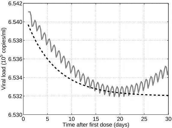
Fig. 6.1. Viral load following standard treatment protocol of 300 mg per day (solid line) and decaying exponential target for control scheme (dashed line).

a baseline) that approximates the first 20 days of standard treatment, as indicated in Figure 6.1.

Starting with an initial dose, ˆu, corresponding to a treatment schedule of 150 mg daily the iterative scheme produces a dosing schedule shown in Figure 6.2, which results in the viral load shown in Figure 6.3. Starting from other constant levels for the initial dose does not significantly affect the final control obtained. The iterative scheme was also applied to the target given by

˜

yd=φφ†(yd−Czˆ(T)) +Czˆ(T) =φφ†yd+ 1−φφ†Czˆ(T)

so that ˜yd−Czˆ(T)∈ranφ. The dosing schedule returned is not significantly different from that in Figure 6.2 but it is seen that the response converges to the outputyd, as seen in Figure 6.4. This modified target is dependent on the initial dosing schedule, ˆ

u, both in terms of the dependence ofφon ˆz, but also in terms of the presence of the termCzˆ(T).

0 5 10 15 20 25 30 100

200 300 400 500 600 700

Time after first dose (days)

Dose (mg)

Fig. 6.2. Dosing schedule returned by iterative scheme (circles) starting from initial schedule of 150 mg per day (squares).

Application of the Contraction Mapping Theorem yields a constructive method to determine the required fixed point solution, and from this the required control is obtained. However, this approach involves integral equations that require the full solution trajectory at each step to be stored. Therefore, an alternative, more direct, approach was presented, in which an iterative scheme for the control is implemented that uses the original system dynamics. The same conditions for the fixed point approach are required and the iterative scheme yields the same solution, though in this case the required control is directly constructed. If a solution to the original problem exists, which yields the required target trajectory, it remains to be determined whether the fixed point approach presented here determines it.

The applicability of the iterative scheme for constructing the required control was illustrated by considering the problem of determining a dosing schedule for the control of HIV dynamics. The model for the viral dynamics of HIV in patients proposed by Dixit and Perelson [5] includes an intracellular delay parameter and was coupled with a two compartment model for the pharmacokinetics of a reverse transcriptase inhibitor, via saturable nonlinear pharmacodynamic term relating efficacy (within the HIV dynamics model) to plasma drug concentration. Exploiting the time-delay form of the equations a series of oral drug administrations was included in the initial state of the system model. The control produced by the iterative scheme drove the system to a particular trajectory corresponding to the orthogonal projection of the target onto the range of the linear operator plus the orthogonal projection of the output corresponding to the initial control onto the orthogonal complement of the range.

REFERENCES

0 5 10 15 20 25 30 6.530

6.532 6.534 6.536 6.538 6.540 6.542

Time after first dose (days)

Viral load (10

5 copies/ml)

Fig. 6.3.Decaying exponential target for control scheme (dashed black line), viral load following initial dosing schedule of 150 mg per day (solid black line), and viral load following dosing schedule produced by iterative scheme (solid grey line).

0 5 10 15 20 25 30

6.530 6.532 6.534 6.536 6.538 6.540 6.542

Time after first dose (days)

Viral load (10

5 copies/ml)

Mathematical Control and Information, 5 (1988), pp. 41–67.

[2] L. Collatz,Functional analysis and numerical mathematics, Academic Press, New York, 1966. [3] R.F. Curtain and H.J. Zwart,An Introduction to Infinite-Dimensional Linear Systems

The-ory, Springer-Verlag, 1995.

[4] E.J. Davison and E.C. Kunze,Some sufficient conditions for the global and local

controlla-bility of nonlinear time varying systems, SIAM Journal on Control, 8 (1970), pp. 489–497.

[5] N.M. Dixit and A.S. Perelson,Complex patterns of viral load decay under antiretroviral

ther-apy: influence of pharmacokinetics and intracellular delay, Journal of Theoretical Biology,

226 (2004), pp. 95–109.

[6] N.D. Evans,Optimal oral drug dosing via application of the contraction mapping theorem, Biomedical Signal Processing and Control, 6 (2011), pp. 57–63.

[7] N.D. Evans and A.J. Pritchard,A control theoretic approach to containing the spread of

rabies, IMA Journal of Mathematics Applied in Medicine and Biology, 18 (2001), pp. 1–23.

[8] H. Hermes,Controllability and the singular problem, Journal of the Society for Industrial and Applied Mathematics, Series A: Control, 2 (1964), pp. 241–260.

[9] D. Hinrichsen and A.J. Pritchard,Robust stability of linear evolution operators on Banach

spaces, SIAM Journal on Control and Optimization, 32 (1994), pp. 1503–1541.

[10] S.G. Krein,Linear Differential Equations in Banach Space, vol. 29 of Translations of Mathe-matical Monographs, American MatheMathe-matical Society, Providence, RI, 1971.

[11] K. Magnusson and A.J. Pritchard,Local exact controllability of nonlinear evolution

equa-tions, in Recent advances in differential equations, R. Conti, ed., Academic Press, London,

1981, pp. 271–280.

[12] K. Magnusson, A.J. Pritchard, and M.D. Quinn,The application of fixed point theorems

to global nonlinear controllability problems, in Mathematical Control Theory, C. Olech,

B. Jakubczyk, and J. Zabczyk, eds., vol. 14 of Banach Center Publications, PWN-Polish Scientific Publishers, Warsaw, 1985, pp. 319–344.

[13] M.-J. Mhawej, C.H. Moog, F. Biafore, and C Brunet-Franc¸ois,Control of the hiv

infec-tion and drug dosage, Biomedical Signal Processing and Control, 5 (2010), pp. 45–52.

[14] M.Z. Nashed, Generalised inverses, normal solvability, and iteration for singular operator

equations, in Non-linear functional analysis and its applications, L. B. Rall, ed., Academic

Press, 1971, pp. 311–359.

[15] A. Pazy,Semigroups of Linear Operators and Applications to Partial Differential Equations, Springer-Verlag, New York, 1983.

[16] A.J. Pritchard and D. Salamon,The linear quadratic control problem for infinite

dimen-sional systems with unbounded input and output operators, SIAM Journal on Control and

Optimization, 25 (1987), pp. 121–144. [17] H. Tanabe,Equations of Evolution, Pitman, 1979.