warwick.ac.uk/lib-publications
Original citation:
Veras, Dimitri. (2016) Post-main-sequence planetary system evolution. Royal Society Open
Science , 3 (2). 150571.
Permanent WRAP URL:
http://wrap.warwick.ac.uk/78568
Copyright and reuse:
The Warwick Research Archive Portal (WRAP) makes this work of researchers of the
University of Warwick available open access under the following conditions.
This article is made available under the Creative Commons Attribution 4.0 International
license (CC BY 4.0) and may be reused according to the conditions of the license. For more
details see: http://creativecommons.org/licenses/by/4.0/
A note on versions:
The version presented in WRAP is the published version, or, version of record, and may be
cited as it appears here.
rsos.royalsocietypublishing.org
Review
Cite this article:Veras D. 2016
Post-main-sequence planetary system evolution.R. Soc. open sci.3: 150571. http://dx.doi.org/10.1098/rsos.150571
Received: 23 October 2015 Accepted: 20 January 2016
Subject Category:
Astronomy
Subject Areas:
extrasolar planets/astrophysics/solar system
Keywords:
dynamics, white dwarfs, giant branch stars, pulsars, asteroids, formation
Author for correspondence:
Dimitri Veras
e-mail:[email protected]
Post-main-sequence
planetary system evolution
Dimitri Veras
Department of Physics, University of Warwick, Coventry CV4 7AL, UK
The fates of planetary systems provide unassailable insights into their formation and represent rich cross-disciplinary dynamical laboratories. Mounting observations of post-main-sequence planetary systems necessitate a complementary level of theoretical scrutiny. Here, I review the diverse dynamical processes which affect planets, asteroids, comets and pebbles as their parent stars evolve into giant branch, white dwarf and neutron stars. This reference provides a foundation for the interpretation and modelling of currently known systems and upcoming discoveries.
1. Introduction
Decades of unsuccessful attempts to find planets around other Sun-like stars preceded the unexpected 1992 discovery of planetary bodies orbiting a pulsar [1,2]. The three planets around the millisecond pulsar PSR B1257+12 were the first confidently reported extrasolar planets to withstand enduring scrutiny due to their well-constrained masses and orbits. However, a retrospective historical analysis reveals even more surprises. We now know that the eponymous celestial body that Adriaan van Maanen observed in the late 1910s [3,4] is an isolated white dwarf (WD) with a metal-enriched atmosphere: direct evidence for the accretion of planetary remnants.
These pioneering discoveries of planetary material around or in post-main-sequence (post-MS) stars, although exciting, represented a poor harbinger for how the field of exoplanetary science has since matured. The first viable hints of exoplanets found around MS stars (γ Cephei Ab and HD 114762 b) [5,6], in 1987–1989, were not promulgated as such due to uncertainties in the interpretation of the observations and the inability to place upper bounds on the companion masses. A confident detection of an MS exoplanet emerged with the 1995 discovery of 51 Pegasi b [7], followed quickly by 70 Virginis b [8] and 47 Ursae Majoris b [9], although in all cases the mass degeneracy remained. These planets ushered in a burgeoning and flourishing era of astrophysics. Now, two decades later, our planet inventory numbers in the thousands; over 90% of all known exoplanets orbit MS stars that will eventually become WDs, and WDs will eventually become the most common stars in the Milky Way.
2
rsos
.ro
yalsociet
ypublishing
.or
g
R.
Soc
.open
sc
i.
3
:1
5057
[image:3.522.66.448.36.554.2]1
...
abbreviations: section 1: Introduction
section 2: Stellar evolution key points 2.1: Single star evolution
2.2: Common envelope and binary star evolution section 3: Observational motivation
3.1: Planetary remnants in and around WDs 3.2: Major and minor planets around WDs 3.3: Subgiant and giant star planet systems 3.4: Putative planets in post-CE binaries
AGB: asymptotic giant branch CE: common envelope GB: giant branch MS: main sequence NS: neutron star RGB: red giant branch SB: substellar body SN: supernova WD: white dwarf 3.5: Pulsar planets
3.6: Circumpulsar asteroid and disc signatures section 4: Stellar mass ejecta
4.1: The mass-variable point-mass two-body problem 4.2: The mass-variable solid body two-body problem 4.3: Stellar wind/gas/atmospheric drag
section 5: Star–planet tides 5.1: Tidal theory
often-used variables:
5.2: Simulation results section 6: Stellar radiation
6.1: Giant branch radiation 6.2: Compact object radiation section 7: Multi-body interactions
7.1: Collisions within debris discs
a semimajor axis e eccentricity
G gravitational constant i inclination
L luminosity M mass
r distance R radius
t time T temperature v velocity r density 7.2: One star, one planet and asteroids
7.3: One star, multiple planets and no asteroids subscripts: 7.4: Two stars, planets and no asteroids
7.5: Two stars, one planet and asteroids 7.6: Three stars only
section 8: Formation from stellar fallback
none mutual property of SB and star star
b binary stellar companion d disc
8.1: Post-CE formation around WDs 8.2: Post-SN formation around NSs
8.3: Formation from tidal disruption of companions section 9: WD disc formation from 1st-GEN SBs section 10: WD disc evolution
section 11: Accretion onto WDs section 12: Other dynamics
section 13: The fate of the solar system section 14: Numerical codes
section 15: Future directions 12.1: General relativity
15.1: Pressing observations 15.2: Theoretical endeavours 12.2: Magnetism
12.3: External influences 12.4: Climate and habitability
disambiguation equations: 2.3: initial-to-final mass relation 2.4: WD radius-to-mass relation 2.5: WD luminosity-to-mass relation 3.2: probability of transit or occultation 3.3: duration of transit or occultation 4.12: semimajor axis change from SN 4.13: escape condition from SN 4.14: eccentricity change from SN 4.16: accretion rate onto SB 4.20: gravitational drag force 4.21 + 10.8: frictional drag force 5.1: semimajor axis evolution from tides 6.1: orbital evolution from stellar radiation 9.1: tidal disruption radius
GB WD
fr
ont matter
body
end matter
NS
Figure 1.Paper outline and nomenclature. Some section titles are abbreviated to save space. Variables not listed here are described in
situ, and usually contain descriptive subscripts and/or superscripts. The important abbreviation ‘substellar body’ (SB) can refer to, for example, a brown dwarf, planet, moon, asteroid, comet or pebble. ‘Disambiguation equations’ refer to relations that have appeared in multiple different forms in the literature. In this paper, these other forms are referenced in the text that surrounds these equations, so that readers can decide which form is best to use (or newly derive) for their purposes. Overdots always refer to time derivatives. The expression
refers to averaged quantities.
3
rsos
.ro
yalsociet
ypublishing
.or
g
R.
Soc
.open
sc
i.
3
:1
5057
[image:4.522.57.465.42.489.2]1
...
mass ejecta orbital changes section 4
mass ejecta physical changes section 4
star–planet tides section 5 stellar radiation
section 6 general relativity
section 12a magnetic fields
section 12b galactic tides
section 12c stellar flybys
section 12c
distance in AU 10–3 10–2
giant branch (GB) phases
10–1 1 10 102 103 104 105
mass ejecta orbital changes section 4
mass ejecta physical changes section 4
star–planet tides section 5 stellar radiation
section 6 general relativity
section 12a magnetic fields
section 12b galactic tides
section 12c stellar flybys
section 12c distance in AU
definitely non-negligible for at least some substellar bodies (SBs)
possibly non-negligible for at least some substellar bodies (SBs)
negligible for all substellar bodies (SBs) 10–3 10–2
white dwarf (WD) and neutron star (NS) phases
10–1 1 10 102 103 104 105
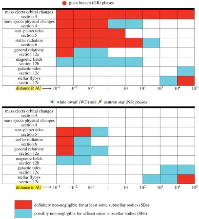
Figure 2.Important forces in post-MS systems. These charts represent just a first point of reference. Every system should be treated on
a case-by-case basis. Magnetic fields include those of both the star and the SB, and external effects are less penetrative in the GB phases because they are relatively short.
Post-MS planetary system investigations help alleviate these uncertainties, particularly with escalating observations of exoplanetary remnants in WD systems. Unlike for pulsar systems, planetary signatures are common in and around WD stars. The exquisite chemical constraints on rocky planetesimals that are gleaned from WD atmospheric abundance studies is covered in detail by the review of Jura & Young [17], and is not a focus of this article. Similarly, I do not focus on the revealing observational aspects of the nearly forty debris discs orbiting WDs, a topic recently reviewed by Farihi [18].
4
rsos
.ro
yalsociet
ypublishing
.or
g
R.
Soc
.open
sc
i.
3
:1
5057
[image:5.522.58.477.63.289.2]1
...
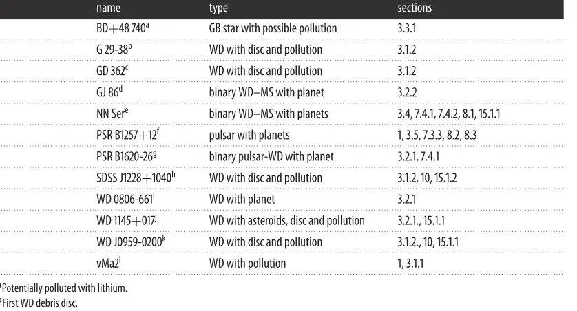
Table 1.Some notable post-MS planetary systems.
name type sections
BD+48 740a GB star with possible pollution 3.3.1
. . . .
G 29-38b WD with disc and pollution 3.1.2
. . . .
GD 362c WD with disc and pollution 3.1.2
. . . .
GJ 86d binary WD–MS with planet 3.2.2
. . . .
NN Sere binary WD–MS with planets 3.4, 7.4.1, 7.4.2, 8.1, 15.1.1
. . . .
PSR B1257+12f pulsar with planets 1, 3.5, 7.3.3, 8.2, 8.3
. . . .
PSR B1620-26g binary pulsar-WD with planet 3.2.1, 7.4.1
. . . .
SDSS J1228+1040h WD with disc and pollution 3.1.2, 10, 15.1.2
. . . .
WD 0806-661i WD with planet 3.2.1
. . . .
WD 1145+017j WD with asteroids, disc and pollution 3.2.1., 15.1.1
. . . .
WD J0959-0200k WD with disc and pollution 3.1.2., 10, 15.1.1
. . . .
vMa2l WD with pollution 1, 3.1.1
. . . .
aPotentially polluted with lithium. bFirst WD debris disc.
cPolluted with 17 different metals. dPlanet orbits the MS star. eMultiple circumbinary planets. fFirst confirmed exoplanetary system. gFirst confirmed circumbinary planet. hDisc probably eccentric and axisymmetric. iPlanet at several thousand astronomical units. jOnly WD with transiting SBs, a disc and pollution. kHighly variable WD disc.
lFirst polluted WD.
1.1. Article layout
I begin by providing a visual table of contents infigure 1, which includes handy references for the abbreviations and commonly used variables in this article. I use the abbreviation ‘SB’ (‘substellar body’ or ‘smaller body’) extensively in the text and equations; constraining relations to just one of planets, asteroids, comets or pebbles is too restrictive for the strikingly diverse field of post-MS planetary science. The term also includes brown dwarfs, for which many physical relations presented here also apply. ‘Planetary systems’ is defined as systems which include SBs. The ‘disambiguation’ equations identified infigure 1refer to relations that have appeared in multiple different forms in the previous post-MS planetary literature; I attempt to consolidate these references. Infigure 2, I characterize distances from the star in which various forces are important, or might be important. This figure may be used as a guide when modelling a particular system or set of systems.Table 1lists some notable post-MS planetary systems, along with brief descriptions and pointers to where they are mentioned in the text.
My deliberately basic treatment of introductory material (stellar evolution and observations from §§2 to 3) is intended to provide the necessary background for subsequent sections, and not meant to emulate an in-depth synopsis. The body of the article (§§4–12) provides more detail on the dynamical aspects of post-MS planetary science. This review concludes with brief comments on the fate of the Solar system (§13), a hopefully helpful summary of the numerical codes that have or may be used in theoretical investigations (§14) and a promising outlook on the future of this science (§15), with guidance for how upcoming observations can maximize scientific return.
2. Stellar evolution key points
5
rsos
.ro
yalsociet
ypublishing
.or
g
R.
Soc
.open
sc
i.
3
:1
5057
1
...
to provide the necessary information for post-MS planetary system studies; for more detail, see e.g. [19,20].
2.1. Single star evolution
2.1.1. Main sequence
The MS evolution is important because it provides the historical context and initial conditions for dedicated post-MS studies. MS stars quiescently burn hydrogen to produce helium in their cores, and do lose mass through winds according to eqn 4 of [21] and eqn 9 of [22]. The Sun currently loses mass at a rate of about 2.4×10⁻¹⁴Myr−1(p. 15 of [23]). The MS lifetime is sensitively dependent on the initial value ofM(MS) and less so on the star’s metallicityZ. This lifetime decreases drastically (by two orders of magnitude, from about 10 to 0.1 Gyr) as the initial mass increases from 1 to 6M(see fig. 5 of [24]).
2.1.2. Giant branches
All stars experience the ‘red giant branch’ (RGB) phase, when hydrogen in the core is exhausted and the remaining hydrogen burns in a contracting shell as the envelope expands. The extent of convection in the star increases, potentially ‘dredging-up’ already-burnt matter. Eventually, core temperatures become high enough to burn helium. For stars withM(MS) <2.0M, helium ignition sets off so-called ‘helium flashes’. This value of 2.0M represents a key transition mass; the duration and character of the mass loss changes markedly when crossing this threshold. After the core helium is exhausted, a helium-burning shell is formed. At this point, the star is said to have begun evolving on the ‘asymptotic giant branch’ (AGB). Another expansion of convection may then cause a ‘second dredge-up’. When, during the AGB, the helium-burning shell reaches the hydrogen outer envelope, a different type of helium flash occurs (denoted a ‘thermal pulse’), one which emits a sudden burst of luminosity and mass. This event, which can occur many times, also causes a sudden increase and then drop in stellar radius (see fig. 3 of [25]). Therefore, AGB thermal pulses literally cause the star to pulsate. Changes in the star’s convective properties during this violent time may also allow for a ‘third dredge-up’ to then occur.
During both the RGB and AGB phases, the star undergoes significant mass loss (up to 80%), radius variability (up to about 10 AU, from an initial value of 10−3−10−2AU), and luminosity variability (up
to many tens of thousand times the MS value) regardless of the extent of the pulses.Figure 3provides representative values; the highlighted rows indicate the most typical progenitors for the currently observed Milky Way WD population. These changes along the GB phases may completely transform a planetary system; indeed linking WD and MS planetary systems is a goal and a challenge, and may also help constrain stellar evolution. Unfortunately, identifying the dominant mechanisms responsible for mass loss—both isotropic and anisotropic—on the RGB and AGB continues to prove difficult.
Red giant branch mass loss.On the RGB, mass-loss is traditionally parametrized by the Reimers formula, a series of proportionalities that was later calibrated [28] and recently improved upon [29] to finally give
dM(RGB)
dt =8×10
−14M yr−1
L(RGB)
L
R(RGB)
R
M(RGB)
M
−1
×
T(RGB) 4000 K
7/2⎡
⎣1+2.3×10⁻⁴
g(RGB) g
−1⎤
⎦, (2.1)
wheregrefers to surface gravity. Traditional formulations of equation (2.1), which are still widely used, do not include the final two terms, and have a leading coefficient of 2×10⁻¹³Myr−1.
Asymptotic giant branch mass loss.Applying the Reimers formula on the AGB can produce significantly erroneous results (fig. 13 of [30]). Instead, during this phase a different prescription is often applied, whose formulation [31] has stood the test of ongoing observations and can be found, for example, in eqns 2–3 of [32]. Accompanying each AGB pulse is a variation in mass loss of potentially a few orders of magnitude, a phenomenon now claimed to have been observed [33]. At the final stage of the AGB— ‘the tip’ of the AGB—the wind is particularly powerful and is known as the ‘superwind’ (e.g. [34]). A star’s peak mass loss rate typically occurs during the superwind unless the AGB phase is non-existent or negligible.
6
rsos
.ro
yalsociet
ypublishing
.or
g
R.
Soc
.open
sc
i.
3
:1
5057
[image:7.522.122.403.40.373.2]1
...
MS stellar
type
B3 6.30 1.18 6.19 9.27 × 10⁻⁵ 66200 0.086 0.92 2.0 × 10⁻⁴
B4 5.00 1.00 4.98 6.51 × 10⁻⁵ 46100 0.25 1.41 2.5 × 10⁻⁴
B5 4.30 0.91 4.29 5.15 × 10⁻⁵ 35900 0.49 1.89 3.0 × 10⁻⁴
B8 3.00 0.75 2.86 2.78 × 10⁻⁵ 18700 2.42 4.19 4.5 × 10⁻⁴
A0 2.34 0.65 2.26 2.33 × 10⁻⁵ 12700 7.71 5.72 6.0 × 10⁻⁴
A5 2.04 0.64 1.86 1.88 × 10⁻⁵ 9500 20.0 6.27 1.4 × 10⁻³
F0 1.66 0.60 1.55 1.32 × 10⁻⁵ 7140 88.0 5.24 0.040
F5 1.41 0.57 1.35 9.56 × 10⁻⁶ 5800 220 5.08 0.11
G0 1.16 0.53 1.15 1.14 × 10⁻⁵ 4520 536 4.82 0.41
G2 1.11 0.53 1.11 7.44 × 10⁻⁶ 4300 621 4.77 0.57
G5 1.05 0.52 1.07 6.89 × 10⁻⁶ 4130 684 4.77 0.82
K0 0.90 0.51 0.92 2.07 × 10⁻⁷ 3590 888 5.01 4.14
MS mass
WD mass
(M) (M) max AGB radius (AU)
max mass loss
rate (M/yr)
max lum-inosity
(L) RGB
time span (Myr)
AGB time span (Myr)
RGB mass loss/ AGB mass
loss
Figure 3.Useful values for 12 different stellar evolution tracks. I mapped the first column to the second by using appendix B of [26], and
then created the remaining columns by using theSSEcode [27] by assuming its default values (which includes Solar metallicity). The four highlighted rows roughly represent the range of the most common progenitor stars for the present-day WD population in the Milky Way.
studies is [35]
vwind=
2GM
R
⎛
⎝1−[v(rot)]2R
GM sin
2θ
⎞
⎠, (2.2)
whereθis the stellar co-latitude andv(rot)is the stellar rotational speed at the equator.
Giant branch changes from substellar body ingestion. If a large SB such as a brown dwarf of planet is ingested during the GB phases, two significant events might result: an enhancement of lithium in the photosphere and spin-up of the star. The former was predicted in 1967 by Alexander [36]. Adamówet al. [37] claimed that SB accretion onto stars can increase their Li surface abundance for a few Myr. However, an enhanced abundance of Li in GB stars could also indicate dredge-up by the Cameron–Fowler mechanism, mixing through tides, or thermohaline or magneto-thermohaline processes. Therefore, a planetary origin interpretation for Li overabundance remains degenerate.
Several investigations have considered how a GB star spins up due to SB accretion. In his eqn 1, Massarotti [38] computed the change in the star’s rotational speed. He suggested that a population of GB fast-rotators due to planet ingestion would be detectable if the speed increased by at least 2 km s−1. Carlberget al.[39] found that a few percent of the known population of exoplanets (at the time) could create rapid rotators, where rapid is defined as having a rotational speed larger than about 10 km s−1.
7
rsos
.ro
yalsociet
ypublishing
.or
g
R.
Soc
.open
sc
i.
3
:1
5057
1
...
AGB envelopes for this or other purposes, one may use a power-law density profile (see, e.g. Sec. 2 [45]); Willes & Wu [46] instead gave a more complex form in their eqn 5.
2.1.3. White dwarfs
For stars with M(MS) 8M, after the GB envelope is completely blown away the remaining core becomes a WD [27,47,48]. In the Milky Way, about 95% of all stars will become WDs [47]. The term ‘white’ in WD originates from the notion that the majority of known WDs are hotter than the Sun [47]. The expelled material photoionizes and the resulting observed structure, which might not have any relation to planets whatsoever, is confusingly termed a ‘planetary nebula’. Although the expelled material will encounter remnant planets and asteroids, few investigations so far have tried to link these nebulae with planets. Even the link between nebula morphology and stellar configurations remains uncertain [49] although SBs that are at least as massive as planets, as well as stellar-mass companions, are thought to play a significant role in shaping and driving the nebulae (e.g. [50,51]).
The time elapsed since the moment an AGB star becomes a WD is denoted the ‘cooling age’ because the WD is in a state of monotonic cooling (as nuclear burning has now stopped). The term cooling age allows one to distinguish from the total age of the star, which includes its previous evolutionary phases. Although some investigations refer to planetary nebula or ‘post-AGB’ as the name of a separate stellar evolutionary phase [52,53], I do not, and assume that the transition from AGB to WD contains no other evolutionary phase.
White dwarf designations.WDs have and continue to be characterized observationally by the dominant spectral absorption lines in their atmospheres. These designations [54] include ‘D’, which stands for degenerate, ‘A’, for hydrogen rich, ‘B’ for helium rich, ‘Z’ for metal-rich (metals are elements heavier than helium) and ‘H’ for magnetic. About 80–85% of the WD population are DA WDs [47,48]. Non-DA WDs probably lost their hydrogen in a relatively late-occurring shell flash.
White dwarf composition.The composition of the WD core is some combination of carbon (from the burning of helium), oxygen (from the burning of carbon) and rarely neon (from the burning of oxygen). The vast majority of WD cores contain carbon and oxygen because they are not hot enough to host copious quantities of oxygen and neon. Only trace amounts of other metals should exist.
White dwarf mass.The initial mass function combined with the current age of the Galaxy has conspired to yield a present-day distribution of WD masses according to fig. 2 of [47] and figs 8, 10 and 11 of [55]. These figures indicate a unimodal distribution that is peaked at about 0.6M and contains a long tail at masses higher than 0.8M. This distribution also conforms with a previous large (348 objects) survey [56], where 0.4M and 0.8M values are considered to be ‘low-mass’ and ‘high-mass’ [57]. In principle, WD masses can range up to about 1.4M. Only single stars with M(MS) 0.8M could have already become WDs, and hence single WDs must have masses that satisfyM(WD) 0.4M. For comparable or lower mass single WDs, perhaps substellar companions could have stripped away some of this mass during the CE phase [58].
How the mass of a WD is related to its progenitor MS mass represents an extensive field of study characterized by the ‘initial-to-final-mass relation’. Observationally, this relation is often determined with WDs that are members of stellar clusters whose ages are well constrained. However, the relation is dependent on stellar metallicity, and in particular the chemistry of individual stars. Ignoring those dependencies, some relations used in the post-MS planetary literature include eqn 6 of [59] (originally from [60]), eqn 9 of [61] (originally from [21]) and eqn 6 of [62] (originally from [63]).
One study which did evaluate how the initial–final mass relationship is a function of metallicity is Menget al.[64]. They found that metallicity can change the final mass by 0.4M, a potentially alarming variation given the difference between a ‘low-mass’ WD (0.4M) and a ‘high-mass’ WD (0.8M). Meng et al. [64] also provided in their appendix potentially useful WD–MS mass relations as a function of metallicity, for Z=[0.0001, 0.0003, 0.001, 0.004, 0.01, 0.02, 0.03, 0.04, 0.05, 0.06, 0.08, 0.1]. For Solar metallicity (Z=Z=0.02) and any star that will become a WD for 0.8M<M(MS) <6.0M, they found
M(WD)
M =min
⎡
⎣0.572−0.046M(MS)
M +0.0288
M(MS)
M
2
, 1.153−0.242M
(MS)
M +0.0409
M(MS)
M
2⎤
⎦.
(2.3)
White dwarf radius. Usefully for modellers, the radius of the WD can be estimated entirely in terms of M(WD) with explicit formulae. A particularly compact but broad approximation is R(WD) /R∼10−2(M(WD)
8
rsos
.ro
yalsociet
ypublishing
.or
g
R.
Soc
.open
sc
i.
3
:1
5057
1
...
that the WD temperature is zero—that are within a few percent of one another are from eqn 15 of [65], and, as shown below, eqns 27–28 of [66]:
R(WD)
R ≈0.0127
M(WD)
M
−1/3
1−0.607M(WD)
M
4/3
. (2.4)
From equation (2.4), I obtain a canonical WD radius of 8750 km=0.0126R, assuming the fiducial value ofM(WD) =0.6M.
White dwarf luminosity. The luminosity of WDs can be estimated in multiple ways. A rough approximation that does not include dependencies on stellar mass or metallicity is from eqn 8 of [67], which is originally from Althauset al.[68]:L=L(tcool=0)×[tcool/105years]−1.25, wheretcoolis the WD
cooling age. I include these dependencies by combining the prescription originally from Mestel [69] with expressions used in post-MS planetary contexts from eqn 6 of [32] and eqn 5 of [70] to obtain
L(WD) =3.26L
M(WD) 0.6M
Z 0.02
0.4
0.1+ tcool Myr
−1.18
, (2.5)
whereZis the assumed-to-be-fixed stellar metallicity. Depending on the WD cooling age, the star’s luminosity can range from about 103Lto 10−5L. This formula also applies only until ‘crystallization’ sets in, which occurs forT(WD)6000–8000 K [71].
2.1.4. Neutron stars
For stars withM(MS) 8M, the end of the AGB phase results in an explosion: a core collapse plus an outwardly expanding shockwave that nearly instantaneously (with velocities of approx. 103− 104km s−1) expels the envelope and causes the star to lose at least half of its mass. This event is a supernova (SN). Any asymmetry in the SN will cause a velocity ‘kick’. The remaining stellar core becomes either a neutron star (NS) or a black hole. Of most relevance to post-MS planetary science are pulsars, which are an august class of NSs that represent precise, stable and reliable clocks.
Although NSs and WDs are together grouped as ‘compact stars’, NSs are much more compact, with radii on the order of 10 km. NS masses are greater than those of WD stars. TypicallyM(NS) ≥1.4M. NSs cool much faster than WDs, with a decreasing luminosity which can be modelled by (p. 30 of [72])
L(NS) =0.02L
M(NS)
M
2/3
max(tcool, 0.1 Myr)
Myr
, (2.6)
wheretcoolrepresents the NS cooling time in this context.
Millisecond pulsars have rotational periods on the order of milliseconds. They are thought to have been spun up by accretion, and are hence said to be ‘recycled’. Miller & Hamilton [73] argued that the presence of planets around millisecond pulsars can constrain the evolutionary history of the star. In particular, they posed that the moon-sized SB around the millisecond pulsar PSR B1257+12 demonstrates how that particular star is not recycled by (i) favouring a second-generation formation scenario for the SB (see §8) and (ii) suggesting that the formation cannot have occurred during an accretional event nor in a post-spin-up disc. They claimed that the moon-sized SB must have formed, post-SN, around the star as is with its current rotational frequency and magnetic moment.
2.2. Common envelope and binary star evolution
Stellar binary systems are important because they represent several tens of percent of all Milky Way stellar systems. The presence of a stellar binary companion can significantly complicate the evolution if the mutual separation is within a few tens of AU. Both star–star tides and the formation of a ‘common envelope’ (CE) can alter the fate otherwise predicted from single-star evolution. Ivanova et al. [74] reviewed the theoretical work performed on and the physical understanding of CEs; see their fig. 1 for some illustrative evolutionary track examples. Taam & Ricker [75] provided a shorter, simulation-based review of the topic.
9
rsos
.ro
yalsociet
ypublishing
.or
g
R.
Soc
.open
sc
i.
3
:1
5057
1
...
the envelope during inspiral. Relevant equations describing this process include eqn 17 of [76], eqns 2– 5 of [77] and eqn 8 of [78]. A more complete treatment that takes into account shock propagation and rotation may be found in eqns 6–25 of [77]; also see the earlier work by [79]. The more massive the companion, and the more extended the envelope, the more likely ejection will occur. The speed of infall within the CE may be expressed generally as a quartic equation in terms of the radial velocity (eqn 9 of [51]), but only if the SB’s tangential velocity is known, as well as the accretion rate onto the SB. Eqn 1 of [58] approximates the final post-CE separation after inspiral.
Even without a CE, the interaction between both stars might dynamically excite any SBs in that system, particularly when one or both stars leave the MS. Both stars might be similar enough in age (and hence MS mass) to undergo coupled GB mass loss. Section 5.2 of [80] quantified this possibility, and finds that the MS masses of both components must roughly lie within 10% of one another in order for both to simultaneously lose mass during their AGB phases.
3. Observational motivation
Post-MS planetary systems provide multiple insights that are not available from MS planetary systems, including: (i) substantive access to surface and interior SB chemistry, (ii) a way to link SB fate and formation, (iii) different constraints on tidal, mass-losing and radiative processes and (iv) the environments to allow for detections of extreme SBs. The agents for all this insight come from GB, WD and NS planetary systems. Overall, the total number of WD remnant planetary systems is of the same order (approx. 1000) as MS planetary systems, and about one order of magnitude more than GB planetary systems. The number of remnant planetary systems around NSs is a few.
3.1. Planetary remnants in and around white dwarfs
Fragments and constituents of disrupted SBs that were planets, asteroids, moons, comets, boulders and pebbles observationally manifest themselves in the atmospheres of WDs and the debris discs which surround WDs. The mounting evidence for and growing importance of both topics is, respectively, highlighted in recent reviews [17,18]. Here, I devote just one subsection to the observational aspects of each topic.
3.1.1. White dwarf atmospheric pollution
Because WDs are roughly the size of the Earth but contain approximately the mass of the Sun, WDs are about 105as dense as the Sun. Consequently, due to gravitational settling, WD atmospheres quickly separate light elements from heavy elements [81], causing the latter to sink as oil would in water. This stratification of WD atmospheres by atomic weight provides a tabula rasa upon which any ingested contaminants conspicuously stand out—as long as we detect them before they sink.
Composition of intrinsic white dwarf photosphere. The chemical composition of the atmosphere is dependent on (i) how the WD evolved from the GB phase and (ii) the WD’s cooling age. At the end of the AGB phase, the star’s photosphere becomes either hydrogen-rich (DA), helium-rich (DB) or a mixed hydrogen–helium composition (DAB, DBA). The link between spectral type and composition is sometimes not so clear, as more literally a DA WD refers to a WD whose strongest absorption features arise from H, and similarly a DB WD has the strongest absorption features arising from He. If the cooling age is within a few tens of Myr, then the WD is hot enough to still contain heavy elements in the photosphere. These elements are said to be ‘radiatively levitated’. For cooling ages between tens of Myr and about 500 Myr, the atmosphere consists of hydrogen and/or helium only. For cooling ages greater than 500 Myr, some carbon—but usually only carbon—from the core may be dredged up onto the atmosphere. Effectively then, WDs that are older than a few tens of Myr and do not accrete anything have atmospheres which are composed of some combination of hydrogen, helium and carbon only.
Composition of polluted white dwarf photosphere.Yet, we have now detected a total of 18 metals heavier than carbon in WDs with 30 Myrtcool500 Myr. These metals, which are said to ‘pollute’ the WD
10
rsos
.ro
yalsociet
ypublishing
.or
g
R.
Soc
.open
sc
i.
3
:1
5057
[image:11.522.109.424.274.418.2]1
...
108
10–2
1
102
104
106
atmospheric sinking time in yr
H-dominated
DA
He-dominated non-DA
109
white dwarf age (cooling time) in yr 60 Myr
Ca C Fe Mg Si Na
300 Myr 1000 Myr 5000 Myr
Figure 4.Cosmetically enhanced version of fig. 1 of [98]. Shown are the sinking times of six metals in WD atmospheres. These times are
orders of magnitude less than the WD cooling ages. The sinking timescales of DA WDs younger than about 300 Myr are days to weeks.
20 8
6
4
log
10
(
M
/g s
–1)
.
25 000 20 000 15 000 10 000 5000
50 100
white dwarf age (cooling time) in Myr white dwarf temperature in kelvins
500 certain pollution possible pollution
5000 1000
Figure 5.Cosmetically reconstructed version of the top panel of fig. 8 of [96]. The blue downward triangles refer to upper limits. The plot
illustrates that accretion rate appears to be a flat function of WD cooling age: pollution occurs at similar rates for young and old WDs.
in WD spectra (Mg is next) [3,4]. Only about 90 years later, with the availability of high-resolution spectroscopy from the Hubble Space Telescope, plus ground-based observations with Keck, VLT, HST and SDSS, did the floodgates open with the detection of 17 of the above metals all within the same WD (GD 362) [82]. A steady stream of highly metal-polluted WDs has now revealed unique, detailed and exquisite chemical signatures (e.g. [83–89]). Two notable cases [90,91] include a high-enough level of oxygen to indicate that the origin of the pollution consisted of water, a possibility envisaged by e.g. [92]. Planetary origin of pollution. A common explanation for the presence of all these metals is accretion of remnant planetary material. The now-overwhelming evidence includes: (i) the presence of accompanying debris discs (see §3.1.2), (ii) SBs caught in the act of disintegrating around a polluted WD (see §3.2.1), (iii) chemical abundances that resemble the bulk Earth to zeroth order (see e.g. [17]), (iv) a variety of chemical signatures that are comparable to the diversity seen across Solar system meteorite families (see e.g. [17]), (v) the debunking of the possibility of accretion from the interstellar medium (see, e.g. eqns 2–6 and table 3 of [93]) and (vi) the fraction of polluted WD systems, which is 25– 50% [94–96] and hence roughly commensurate with estimates of Milky Way MS planet-hosting systems [97]. This last point is particularly remarkable because metals heavier than carbon will sink (or ‘diffuse’, ‘settle’ or ‘sediment’) through the convection or ‘mixing’ zone quickly (figure 4): in days or weeks for DA WDs younger than about 300 Myr and within Myr for DB WDs. In all cases, the sinking times are orders of magnitude shorter than the WD cooling age. Therefore, we should always expect to detect heavy metal pollution at a level well-under 0.1%.
11
rsos
.ro
yalsociet
ypublishing
.or
g
R.
Soc
.open
sc
i.
3
:1
5057
1
...
planetary architectures can generate comparably high levels of accretion at such late ages? (The first polluted WD, vMa 2, is relatively ‘old’, withtcool=3 Gyr.)
Implications for planetary chemistry and surfaces/interiors.For the foreseeable future, the only reliable way to study the chemistry of SBs will be through spectroscopic observations of their tidally disrupted remnants in WD atmospheres. Samples from Solar system meteorites, comets and planets (including the Earth) allow us to make direct connections to chemical element distributions in WD atmospheres. For example, we know that an overabundance of S, Cr, Fe and Ni indicates melting and perhaps differentiation [83]. Signatures of core and crust formation are imbued in the ratio of iron to siderophiles or refractory lithophiles. Also, in particular, Fe-rich cores, Fe-poor mantles or Al-rich crusts may all be distinguished [99]. A carbon-to-oxygen ratio0.8 would result in drastically different physical setup than the Solar system’s [100]. For more details, see [17].
Implications for planetary statistics.Because polluted WDs signify planetary systems, these stars can be used to probe characteristics of the Galactic exoplanet population. Zuckerman [101] considered the population of polluted WDs which are in wide binary systems, and concluded that a comparable fraction of both single-star and wide binary-star systems with rb1000 AU host planets. For rb1000 AU,
however, the binary planet-hosting fraction is less, implying perhaps that in these cases the binary companion suppresses planet formation or more easily creates dynamical instability.
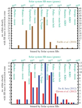
Accumulated metal mass in the convection zone.For DB WDs, the situation is different. Their convection zones are deep enough to hold a record of all remnant planetary accretion over the last Myr or so. This feature allows us to estimate lower bounds for the total amount accreted over this timescale.Figure 6
illustrates the amount of mass in metals, in terms of Solar system asteroids, moons and one L4Jupiter
Trojan, that has been accreted in two different WD samples.
Other constraints. Some metal-polluted WDs are magnetic (denoted with an ‘H’ in the spectral classification). At least 10 DZH WDs harbour magnetic fields of 0.5–10 MG [105], although this preliminary work indicates this number is likely to be double or triple. The theoretical implications of magnetic fields have previously only briefly been touched upon (§12.2).
Further, hydrogen abundance in WD atmospheres, although not considered a ‘pollutant’, nevertheless might provide an important constraint on pollution. Because hydrogen does not diffuse out of a WD atmosphere, this chemical element represents a permanent historical tracer of accretion throughout the WD lifetime (even if the WD’s spectral type changes as a function of time). Accretion analyses and interpretations, however, must assume that the WD begins life with a certain amount of primordial H. This accretion arises from a combination of the interstellar medium, asteroids, comets and any planets. Of these, comets—and in particular exo-Oort cloud comets—might provide the greatest amount of this hydrogen through ices. Consequently, linking WD hydrogen content with cooling age may help determine the accretion rate of exo-Oort cloud comets soon after the WD is formed [67] and over time [106]. Fig. 5 of [91] illustrates how WD hydrogen mass appears to be a steadily increasing function of cooling age, and increases at a rate far greater than realistic estimates of accretion from the interstellar medium.
3.1.2. White dwarf debris discs
Debris discs have been detected orbiting nearly 40 polluted WDs. The first disc discovered orbits the WD Giclas 29–38 (commonly known as G 29–38) [107] in 1987. Nearly two decades passed before the second disc, orbiting GD 362 [108,109], prompted rapid progress. No confidently reported debris disc around a single unpolluted WD exists, suggesting the link between pollution and discs is strong. At least a few percent and up to 100% of all WDs host discs [110–112]. The lower limit for the Galactic population is based on actually observed discs, whereas the one-to-one potential correspondence between pollution and the presence of a disc is based on most discs likely being too faint to detect. Although observational sensitivities allow pollution to be discovered in WDs withtcoolas high as about 5 Gyr, discs are difficult
to detect fortcool>0.5 Gyr [112]. Farihi [18] recently summarized observations of these discs. See also
table 1 of [110], table 1 of [103] and table 2 of [113] for some details of dust-only discs found before 2012. Detection constraints.All these discs are dusty, and dust comprises the major if not sole component. Consequently, the detection and characterization of the discs rely on modelling spectral energy distributions with a signature (‘excess’ with respect to the flux from the WD) in the infrared and a total flux,F, prescription that is given in eqn 3 of [114]:
F≈12π1/3cos (iLOS)R 2
D2
2kBT
3hν
8/3 hν3
c2 x(out)
x(in)
x5/3
12
rsos
.ro
yalsociet
ypublishing
.or
g
R.
Soc
.open
sc
i.
3
:1
5057
1
... 48 45 42 39 36 33 30 27 24 21 18 15 12Farihi et al. (2010) 9 6 3 0 48 45 42 39 36 33 30 27 24 21 18 15 12 9 6 3 0 binned by Solar system SBs
Solar system SB mass (grams)
Phobos
–
moon
1019 1020 1021 1022 1023 1024 1025 1026
Bianca – moon Epimetheus – moon Janus – moon Europa – moon Hektor – L
4 T
rojam Proteus – moon P allas – main belt Ceres – main belt Haumea – K BO Pluto – KBO
no. white dw
arfs
with SB mass in con
v
ection zone
Girven et al. (2012) Xu & Jura (2012)
13 12 11 10 9 8 7 6 5 4 3 2 1 0 13 12 11 10 9 8 7 6 5 4 3 2 1 0
binned by Solar system SBs Solar system SB mass (grams)
Phobos
–
moon
1019 1020 1021 1022 1023 1024 1025 1026
Bianca – moon Epimetheus – moon Janus – moon Europa – moon Hektor – L
4 T
rojan Proteus – moon P allas – main belt Ceres – main belt Haumea – KBO Pluto – KBO
no. white dw
arfs
with SB mass in con
v
ection zone
Figure 6.Histograms of the accumulated mass of rocky substellar bodies that were accreted onto white dwarfs during the last Myr or
so, including both detections and limiting values. Differently coloured bars refer to three different WD samples (brown: data from [93] assuming that Ca represents 1.6% of the mass of the accreted bodies, similar to the corresponding mass fraction of the bulk Earth—see table 3 of [102]; blue: data displayed in fig. 12 of [103]; red: data displayed in fig. 9 of [104]). The panels are separated according to sample size (seey-axis). For observational subtleties associated with the data, see the corresponding papers. The bin sizes are according to the Solar system objects displayed in green, with masses given on the top axis. This plot demonstrates that pollution may arise from a wide variety of objects.
In equation (3.1),ν is the frequency,Dis the distance between the star and the Earth,iLOSis the
line-of-sight inclination with respect to the Earth,kBis the Boltzmann constant,his the Planck constant and
x(r)≡hν/kBTd(r). The discs are assumed to be passive, opaque (optically thick) and geometrically flat.
The equation is degenerate with respect to three parameters:iLOS, and the disc temperatures at the
inner and outer edges. Fig. 5 of [104] and fig. 3 of [115] illustrate how the degeneracy from these three parameters manifests itself in the modelling of debris discs. For an explicit example of how 10 different viewing angles can change the flux signature, see fig. 1 of Livioet al.[57], who simulate the spectral energy distribution for a (so-far unrealized) AU-scale WD debris disc.
Disc characteristics.One such property is disc geometry. The spectral energy distributions generally do not indicate that WD discs are flared. However, a couple of possible exceptions include GD 362 [116] and GD 56 [117]. The size distribution of the dust/particles/solids in the discs is unknown, except for the presence of micrometre-sized grains [118–120]. One notable disc, which orbits WD J0959-0200, is highly variable: Xu & Jura [115] reported a still-unexplained flux decrease of about 35% in under 300 days.
Application of equation (3.1), with assumptions aboutiLOS, yields a striking result for WDs withtcool
13
rsos
.ro
yalsociet
ypublishing
.or
g
R.
Soc
.open
sc
i.
3
:1
5057
1
...
750
500
250
0
Vy
[km s
–1
]
Vx [km s–1]
2016–12
2006–07 2015–06
2012–03
2009–04
–250
–500
–750
750 500 250 0 –250 –500 –750
2003–03
2.0
R
0.2
R
Figure 7.Exact reproduction of fig. 5 of [122]. This image is a velocity space map of the gaseous component of the debris disc orbiting the
WD SDSS J1228+1040. The subscriptsxandyrefer to their usual Cartesian meanings, and the WD is located at the origin. Observations at particular dates are indicated by solid white lines. The image suggests that the disc is highly non-axisymmetric and precessing on decadal timescales.
arose with the discovery of both dusty and gaseous components in seven of these discs. The gaseous components constrain the disc geometry. This distance range clearly demonstrates that (i) the discs do not extend all the way to the WD surface (photosphere) and that (ii) the discs could not have formed during the MS or GB phases. Regarding this first point, some spectral features do suggest the presence of gas within 0.6R(e.g. see the bottom-left panel of fig. 3 in [83]), but not yet in a disc form.
The first gaseous disc component found (around SDSS J122859.93+104032.9, also known as SDSS J1228+1040) [121], also exhibits striking morphological changes, which occur secularly and smoothly over decades (whereas the disc orbital period is just a few hours) [122] (figure 7). The figure is a velocity space intensity distribution where the radial white lines indicate different times from the years 2003– 2016. Four other discs with time-resolved observations of gaseous components are SDSS J0845+2258, SDSS J1043+0855, SDSS J1617+1620 and SDSS J0738+1835. The first three of these—which change shape or flux over yearly and decadal timescales—represent exciting dynamical objects, while the last, which exists in an apparently steady state (given just a handful of epochs so far), might provide an important and intriguing contrast.
One notable exception to all of the above WD discs is a very wide (35–150 AU) dusty structure inferred orbiting the extremely young (tcool 1 Myr) WD 2226-210 [123]. The interpretation of this dusty
annulus representing a remnant exo-Kuiper belt is degenerate and is not favoured compared to a stellar origin [124]: i.e. this annulus might represent a planetary nebula.
3.2. Major and minor planets around white dwarfs
3.2.1. Orbiting white dwarfs
A few WDs host orbiting SBs, and they are all exoplanetary record-breakers (as of time of writing) in at least one way.
The fastest, closest and smallest SBs.Transit photometry of WD 1145+017 revealed signatures of one to several SBs (withRSB<103km) which are currently disintegrating within the WD disruption radius with
14
rsos
.ro
yalsociet
ypublishing
.or
g
R.
Soc
.open
sc
i.
3
:1
5057
1
...
the same system, Xuet al.[128] have detected circumstellar absorption lines from likely gas streams, as well as 11 different metals in the WD atmosphere.
Because this WD is both polluted and hosts a dusty debris disc, these minor planet(s) further confirm the interpretation that accretion onto WDs and the presence of circumstellar discs is linked to first-generation SB disruption (see §9). This type of discovery was foreshadowed by previous prognostications. (i) Soker [129] found that for stars transitioning from the AGB to WD phase, their shocked winds can create mass ablation from surviving planets into a detectable debris tail. (ii) Villaver & Livio [52] predicted that planets evaporating and emitting Parker winds could be detected with spectroscopic observations, but was thinking of atmospheric mass outflows at several AU around GB stars. (iii) Di Stefanoet al.[130] demonstrated specifically that theKeplerspace mission should be able to detect WD transits of minor planets. Ironically, although the paper was written with the primary Keplermission in mind, only during the secondary mission were enough WDs observed to achieve this discovery. (iv) Alternatively, Spiegel & Madhusudhan [131] claimed that the process of a stellar wind accreting onto an SB might produce a detectable coronal envelope around the SB.
The furthest and slowest exoplanet.WD 0806-661 b is a planetary mass (7MJup) SB orbiting the WD at
an approximate distance of 2500 AU [132]. Although some in the literature refer to the object as a brown dwarf, the mass is well constrained to be in the planet regime (see fig. 4 of [132]). The difference of opinions is perhaps partly informed by contrasting assumptions about the SB’s dynamical origin rather than its physical properties. The planet was discovered using direct imaging, and holds the current record for the bound exoplanet with the widest orbit known.
The first circumbinary exoplanet. The first successfully predicted [133,134] and confirmed [135] circumbinary exoplanet, PSR B1620-26AB b, orbits both a WD (with mass≈0.34M and cooling age of approx. 480 Myr) and a millisecond pulsar (with mass≈1.35M and rotation period of 11 ms). The WD cooling age and pulsar rotation period importantly help constrain the dynamical history of the system. The planet’s physical and orbital parameters areMSB∼2.5MJup,a∼23 AU andi∼40◦, whereas
the binary orbital parameters areab≈0.8 AU andeb≈0.025.
PSR B1620-26AB b is the only known planet in a system with two post-MS stars, and one of the few exoplanets ever observed in a metal-poor environment and cluster environment (the M4 globular cluster). The planet name contains ‘PSR’ because the pulsar was the first object in the system discovered and is the most massive object (the primary). However, the planet was originally thought to orbit (and form around) the progenitor of the WD, and hence is more appropriately linked to that star. Further, I do not classify this system as a post-CE binary (see §3.4) because both the system does not fit the definition of containing a WD and a lower-mass MS companion, and the system is typically not included in the post-CE binary literature [136]. This combination of pulsar, WD and planet suggests a particularly fascinating dynamical history (see §7.3.2).
Hints of detections.In addition to the above observations, there are several hints of SBs orbiting WDs. The magnetic WD GD 365 exhibits emission lines which could indicate the presence of a rocky planet with a conducting composition [137]. Later data has been able to rule out an SB withMSB≥12MJup[25],
which is consistent with the rocky planet hypothesis. Also, the spectral energy distribution of PG 0010+280 may be fit with an SB withr≈60 AU [138]. In order for this SB to be hot enough for detection, it may have been re-heated; see their Sec. 3.3.2.
Further, a few tenths of percent of Milky Way WDs host brown dwarf-mass SBs [139]. These companions were found to orbit at distances beyond the tidal engulfment radius of the AGB progenitor of the WD until the notable discovery of WD 0137-349 B [140]. This brown dwarf hasMSB=0.053M. For the primary WD star,M=0.39M. The orbit is close enough—(asiniLOS=0.375R=0.0017 AU)—
that WD 0137-349 B must have survived engulfment in the GB envelope of the progenitor. The low mass of the WD is characteristic of premature CE ejection by a companion.
Search methods.For a recent short summary of the different techniques employed to search for planets around WDs, see Section 1 of [141]. The discovery of SBs orbiting WD 1145+017 based on transit photometry [125] highlights interest in this technique. Faediet al.[142] placed limits (less than 10%) on the frequency of gas giants or brown dwarfs on circular orbits with orbital periods of several hours, and mentioned that exo-moons orbiting WDs can generate 3% transit depths. An important caveat to this transit method is that it requires follow-up with other methods, at least according to [143], who wrote that for WDs, ‘planet detection based on photometry alone would not be credible’.
15
rsos
.ro
yalsociet
ypublishing
.or
g
R.
Soc
.open
sc
i.
3
:1
5057
1
...
estimate the depth of the transit to be equal to unity ifRSB≥Rand, instead, to approximately equal
R2
SB/R2 ifRSB<R. The probability of transit and the duration of transit represent other quantities of
interest. I display these by repackaging the fairly general expressions from eqns 9–10 of [146]:
probability=
R+RSB
a
1±esinω 1−e2
, (3.2)
whereωis the argument of pericentre of the orbit, the upper sign is for transits (SB passing in front of the WD) and the lower sign is for occultations (or ‘secondary eclipses’, when the SB passes in back of the WD). Both formulae assume grazing eclipses, and that eclipses are centred around conjunctions. Maintaining this sign convention, I then combine eqns 7, 8, 14, 15 and 16 of [146] to obtain the transit/occultation duration:
duration=2 1−e2
1+esinω
a3
G(M+MSB)
×sin−1
⎡ ⎣ R
asiniLOS
1±RSB R
2
−a2cos2iLOS(1−e2)2
R2
(1+esinω)2
1/2⎤
⎦, (3.3)
whereiLOSis the inclination of the orbit with respect to the line of sight of an observer on the Earth. By
convention, an edge-on orientation corresponds toiLOS=90◦.
3.2.2. Orbiting the companions of white dwarfs
Three stellar systems are known to harbour a planet-hosting star and a WD: GJ 86,Reticulum (or Ret), and HD 147513. In no case is the WD (yet) known to be polluted nor host debris discs, planets or asteroids.
The star GJ 86B is an unpolluted WD [147] whose binary companion GJ 86A is an MS star that hosts aMSB4.5MJupplanet in ana=0.11 AU orbit [148,149]. With Hubble Space Telescope data, Farihi
et al.[147] helped constrain the physical and orbital parameters of the system (see their table 4), which features a current binary separation of many tens of AU. The planet GJ 86Ab survived the GB evolution of GJ 86B, whenabexpanded by a factor of a few, butebremained fixed (see §4).
A similar scenario holds for the HD 27442 system. The star Ret, or HD 27442A, hosts aMSB
1.6MJup planet in a a=1.27 orbit [150]. The projected separation between Ret and its WD binary
companion, HD 27442B, is approximately a couple hundred AU [151]. The HD 147513 system is not as well constrained [152]. However, the separation between the binary stars in that system is thought to be several thousand AU, placing it in the interesting ‘non-adiabatic’ mass loss evolutionary regime (equation (4.10)).
3.2.3. White dwarf–comet collisions
In the 1980s, the potential for collisions between exo-comets and their parent stars, or other stars, to produce observable signatures was realized [153–155]. Alcocket al.[156] more specifically suggested that comet accretion onto WDs can constrain number of exo-Oort cloud comets in other systems. Pineault & Poisson [155] and Tremaine [157] included detailed analytics that may still be applicable today. Some of this analysis was extended to binary star systems in Pineault & Duquet [158], with specific application to compact objects in their Sec. 4.3. Perhaps, these speculations have been realized with the mysterious X-ray signature from IGR J17361-4441 reported in Del Santoet al.[159], although that potential disruption event may also have just been caused by planets or asteroids rather than comets.
3.3. Subgiant and giant star planetary systems
3.3.1. Giant branch planets
Gross characteristics.As of 30 Nov 2015, 79 SBs were recorded in the planets-around-GB-stars database1, although this number may be closer to 100 [160]. About 85% of these SBs are giant planets withMSB∼1− −13MJup, proving that planets can survive over the entire MS lifetime of their parent stars. The host stars
for these SBs have not undergone enough GB evolution to incite mass loss or radius variations which are markedly different from their progenitor stars. These barely evolved host stars are observed in their early
16
rsos
.ro
yalsociet
ypublishing
.or
g
R.
Soc
.open
sc
i.
3
:1
5057
1
...
RGB phase, sometimes known as the ‘subgiant’ phase. Because RGB tracks on the Hertzprung–Russell diagram are so close to one another, RGB masses are hard to isolate; there is an ongoing debate over the subgiant SB-host masses [161–166].
Regardless, the population of these SBs shows a distinct characteristic: a paucity of planets (less than 10%) within half of an AU of their parent star. In contrast,a<0.5 AU holds true for about three-quarters of all known exoplanets. This difference highlights the need to better understand the long-term evolution of planetary systems. Further, a handful of GB stars have been observed to host multiple planets. These systems may reveal important constraints on dynamical history. For example, the two planets orbiting ηCeti may be trapped in a 2:1 mean motion resonance (see the fourth and fifth rows of plots in fig. 6 of [167]). A resonant configuration during the GB phase would help confirm the stabilizing nature of (at least some types of) resonances throughout all of MS evolution.
Regarding the planet–giant star metallicity correlation, Maldonadoet al.[168] and Reffertet al.[169] arrived at somewhat different conclusions. The former concluded that planet-hosting giant stars are preferentially not metal rich compared to giant stars that do not host planets. The latter, using a different sample, showed that there was strong evidence for a planet—giant star metallicity correlation.
Lithium pollution?One case of particular interest is the BD+48 740 system [37], which contains both (i) a candidate planet with an unusually high planet eccentricity (e=0.67) compared with other evolved star planets and (ii) a host star that is overabundant in lithium. Taken together, these features are suggestive of recent planet engulfment: Lillo-Boxet al.[10] wrote: ‘The first clear evidence of planet engulfment’. They also helped confirm existence of the MS planet Kepler-91b, a tidally-inspiraling extremely close-in planet withr≈1.32R, and estimate that its fate might soon (within 55 Myr) mirror that of the engulfed planet in BD+48 740.
Transit detection prospects. In principle, SBs may be detected by transits around GB stars. The application of equations (3.2 and 3.3) to this scenario is interesting because, as observed by Assef et al.[170], despite the orders of magnitude increase in stellar radius from the MS to GB phases, there is a corresponding increase in values ofafor surviving SBs. Therefore, the transit probability should not be markedly different. The equations neglect however, just how small the transit depth becomes: R2SB/R2∼10−5.
3.3.2. Giant branch debris discs
Importantly, planets are not the only SBs that survive MS evolution. Bonsoret al.[171] revealed the first resolved images of a debris disc orbiting a 2.5 Gyr-old subgiant ‘retired’ A star (κCoronae Borealis orκ CrB), although they could not distinguish between one belt from 20 to 220 AU from two rings or narrow belts at about 40 and 165 AU. This finding demonstrates that either the structure survived for the entire main sequence lifetime, or underwent second-generation formation. This discovery was followed up with a survey of 35 other subgiant stars, three of which (HR 8461, HD 208585 and HD 131496) exhibit infrared excess thought to be debris discs [172]. Taken together, these four disc-bearing GB stars suggest that large quantities of dust could survive MS evolution.
3.4. Putative planets in post-common-envelope binaries
Some binary stars which have already experienced a CE phase are currently composed of (i) either a WD or hot subdwarf star, plus (ii) a lower-mass companion. These binaries are classified as either ‘detached’ or ‘semi-detached cataclysmic variables’ depending on the value ofrb. Over 55 of these binaries have
just the right orientation to our line of sight to eclipse one another. These systems are known as post-CE binaries. The eclipse times in these binaries should be predictable if there are no other bodies in the system and if the stars are physically static objects.
17
rsos
.ro
yalsociet
ypublishing
.or
g
R.
Soc
.open
sc
i.
3
:1
5057
1
...
The most robust detections are the putative planets around the post-CE binary NN Serpentis, or NN Ser. Beuermann et al. [173,174] found excellent agreement with a two-planet fit, and found resonant solutions with true librating angles [174]. A recent analysis of 25 years worth of eclipse timing data for this system (see fig. 2 of [175]) strengthens the planetary hypothesis, particularly because timings between the years of 2010–2015 matched the predicted curve. They do not, however, claim that these planets are confirmed, because there still exists a degeneracy in the orbital solutions. In fact, Mustill et al.[176] provided evidence against the first-generation nature of these planets by effectively backwards integrating in time to determine if the planets could have survived on the MS. The largest uncertainty in their study is not with the orbital fitting but rather how the CE evolved and blew off in that system.
If confirmed, other reported systems which may be dynamically stable would prove exciting. However, pulsation signals, which are intrinsic to the parent star, can mask timing variations that would otherwise indicate the presence of SBs (e.g. [177]). Charpinetet al.[178] detected signals around the hot subdwarf star KIC 05807616 which could correspond to SBs with distances of 0.0060 and 0.0076 AU. Silvottiet al.[179] instead detected timing variations around the subdwarf pulsator KIC 10001893 with periods of 5.3, 7.8 and 19.5 h.
3.5. Pulsar planets
Pulsar arrival timings in systems with a single pulsar are generally better constrained than those in post-CE binaries because pulsars are more reliable clocks than WD or MS stars, and radiation from a single source simplifies the interpretation. Identifying the origin of residual signals for millisecond pulsars is even easier.
These highly precise cosmic clocks, combined with a fortuitous spell of necessary maintenance work on the Arecibo radio telescope, provided Alexander Wolszczan with the opportunity to find PSR B1257+12 c and d [1] (sometimes known as PSR B1257+12 B and C), and eventually later PSR B1257+12 b (sometimes known as PSR B1257+12 A) [2]. Wolszczan [180] detailed the history of these discoveries. Not included in that history is how the identities of the first two planets were almost prematurely leaked by the British newspaperThe Independentin October 1991 [181]. The article referred to these planets as ‘only the second and third planets to be found outside our own solar system’ because of the ironic assumption that the first-ever exoplanet was the (later-retracted [182]) candidate PSR 1829-10 b.
The observed and derived parameters for the PSR B1257+12 system remain among the best
constrained of all exoplanets (see table 1 of [180]), with eccentricity precision to the 10−4level, a value for the mutual inclination of planets c and d (which is about 6 degrees), and a derived mass for planet b of 0.020M⊕=1.6MMoon. However, these values are based on the assumption thatM=1.4M.
PSR B1257+12 b has the smallest mass of any known extrasolar SB, given that we do not yet have well-constrained masses for the (disintegrating) SBs orbiting WD 1145+017. The other two planets are ‘super-Earths’, with masses of planets c and d of 4.3M⊕and 3.9M⊕. All three planets lie within 0.46 AU of the pulsar and travel on nearly circular (e<0.026) orbits. The orbital period ratio of planets b and c is about 1.4759, which is close to the 3:2 mean motion commensurability.
I have already described the one other bona-fide planet discovered orbiting a millisecond pulsar, PSR B1620-26AB b, in §3.2.1, because that planet also orbits a WD. For an alternative and expanded accounting of this planet as well as the PSR B1257+12 system, see the 2008 review of neutron star research [183].
Pulsar planets are rare. A recent search of 151 young (<2 Myr old) pulsars (not ms pulsars) with the Fermitelescope yielded no planets forMSB>0.4M⊕and with orbital periods of under 1 year [184]. The
authors used this result as strong evidence against post-SN fallback second-generation discs (see §8.2), particularly because theoretical models constrain these discs to reside within about 2 AU.
3.6. Circumpulsar asteroid and disc signatures
Sometimes the deviations in pulse timing are not clean in the sense that they cannot be fit with one or a few planets or moon-sized SBs. Rather, the deviations may be consistent with other structures, such as discs, rings, arcs or clouds. Wang [185] recently reviewed observational results from debris disc searches around single pulsars.

![Figure 3. Useful values for 12 different stellar evolution tracks. I mapped the first column to the second by using appendix B of [thencreatedtheremainingcolumnsbyusingthe26], and SSE code[27]byassumingitsdefaultvalues(whichincludesSolarmetallicity).Thefourhighlightedrowsroughlyrepresenttherangeofthemostcommonprogenitorstarsforthepresent-dayWDpopulationintheMilkyWay.](https://thumb-us.123doks.com/thumbv2/123dok_us/9483602.454528/7.522.122.403.40.373/different-evolution-appendix-thencreatedtheremainingcolumnsbyusingthe-byassumingitsdefaultvalues-whichincludessolarmetallicity-thefourhighlightedrowsroughlyrepresenttherangeofthemostcommonprogenitorstarsforthepresent-daywdpopulationinthemilkyway.webp)
![Figure 4. Cosmetically enhanced version of fig. 1 of [98]. Shown are the sinking times of six metals in WD atmospheres](https://thumb-us.123doks.com/thumbv2/123dok_us/9483602.454528/11.522.109.424.274.418/figure-cosmetically-enhanced-version-shown-sinking-metals-atmospheres.webp)
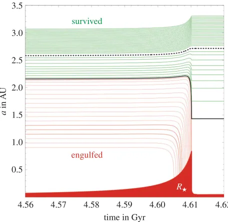
![Figure 9. Cosmetically enhanced version of fig. 3 of [30]. The prospects for survival of Jupiter-mass planets (a) and Earth-mass planets(b)orbitingaAGBstarwithM(MS)⋆= 2.0 M⊙ andevolvingduetotidesandmassloss.Unlikeinfigure8,herethestellarsurfacepulses.(a)Illustrates that surviving Jovian-mass planets must begin their orbits at least 20 per cent further away than the maximum stellar radius.(b) Earth-mass planets with starting orbits that are within the maximum stellar radius can survive.](https://thumb-us.123doks.com/thumbv2/123dok_us/9483602.454528/28.522.87.439.41.222/cosmetically-prospects-orbitingaagbstarwithm-andevolvingduetotidesandmassloss-unlikeinfigure-herethestellarsurfacepulses-illustrates-surviving.webp)
![Figure 10. Cosmetically enhanced version of the lowest panel of fig. 4 of [32]. How GB evolution of a M(MS)⋆= 2.9 M⊙ star depletesa debris disc due to collisional evolution alone](https://thumb-us.123doks.com/thumbv2/123dok_us/9483602.454528/34.522.142.381.40.213/figure-cosmetically-enhanced-version-evolution-depletesa-collisional-evolution.webp)
![Figure 12. Cosmetically enhanced version of the bottom-rightmost panel of fig. 9 of [24]](https://thumb-us.123doks.com/thumbv2/123dok_us/9483602.454528/37.522.141.385.40.205/figure-cosmetically-enhanced-version-rightmost-panel-fig.webp)
