Acoustic Emission Pattern Recognition Method Utilizing Elastic Wave Simulation

Acoustic Emission Pattern Recognition Method Utilizing Elastic Wave Simulation

Kenta Arakawa and Takuma Matsuo

School of Science and Technology, Meiji University, Kawasaki 214–8571, Japan

Fracture mode analysis via acoustic emission (AE) has attracted research attention as a means of identifying the damage mechanism in machines and engineering structures. However, the estimation of relevant parameters from waveforms detected by AE sensors requires com-plex analysis because the waveforms are often distorted by the sensor response. Therefore, in this study, we develop a method for the classifi-cation of AE signals based on simulated AE waveforms. The simulated AE waveform is a convolution of the simulated elastic wave calculated via the 3D finite-difference time-domain (FDTD) method and the sensor response acquired with the use of the long bar method. The AE sig-nals with different propagation angles obtained with the use of an epoxy-glass fiber composite specimen are classified, and wavelet contour maps and correlation coefficients are used for AE classification. The success of the AE classification is validated by the similarity of waveform features between the experiment and simulation. [doi:10.2320/matertrans.M2017104]

(Received April 21, 2017; Accepted July 25, 2017; Published September 1, 2017)

Keywords:  acoustic emission, finite-difference time-domain, pattern recognition, wavelet transform

1.  Introduction

The damage through fracture of machine parts and engi-neering structures can often lead to eventual catastrophic failure. In order to prevent damage of machine parts and structural members under operating conditions, it is import-ant to non-destructively evaluate the physical state and prop-erties of the materials under consideration. In particular, it is necessary to evaluate the occurrence and progress of cracks due to damage phenomena such as fatigue cracks and stress corrosion cracking. In this context, fracture mode analysis via acoustic emission (AE) has attracted increasing attention as an approach to identify the damage mechanism in ma-chines and structures1,2)_{. In particular, AE pattern}

recogni-tion analysis has become a prevalent method to estimate the parameters of the crack mode and crack direction. However, the estimation of these crack parameters from AE wave-forms detected by AE sensors requires complex analysis be-cause the waveforms are often distorted by sensor re-sponse3,4)_{. Furthermore, in a finite specimen, the analysis of}

AE waveforms becomes complex owing to the presence of reflection waves. Consequently, in previous studies on AE waveform simulation, only waveforms detected by wideband sensors and direct signal arrivals have been studied5)_.

To overcome this problem, here, we develop a method for the classification of AE signals based on simulated AE waveforms. The simulated AE waveform is a convolution of a simulated elastic wave and the sensor response signal. The simulated elastic wave is calculated using the 3D finite-dif-ference time-domain (FDTD) method6) _{for application to a}

finite specimen, and the sensor response is experimentally acquired. Here, we note that in our previous study7,8)_,

artifi-cial AE signals were successfully classified by this method. A Hsu–Nielsen source was used to generate artificial AE waveforms by breaking a pencil-lead over a thin aluminum plate. This led to the excitation of artificial AE signals on the surface and side walls of the plate. A contour map of the waveform, generated by wavelet transforms, was used for classification. The correlation coefficient of the contour map

of the waveforms detected in the experiment was compared with that from the simulation and subsequently classified. The characteristics of the simulated waveforms were ob-served to correspond to the artificial AE waveform.

In this study, AE signals (with different propagation an-gles) excited by mode I fractures are classified with the use of an epoxy-carbon composite specimen. The AE signals de-tected during the tensile testing of the specimen are identi-fied and classiidenti-fied for each propagation angle with use of the developed method, and subsequently, we examine the accu-racy of this AE pattern recognition method.

2.  AE Pattern Recognition Method

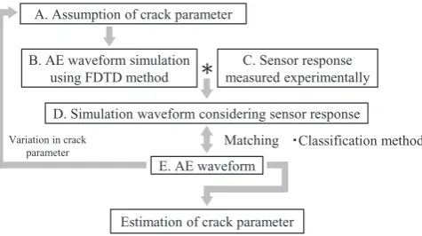
We propose an AE pattern recognition method to estimate the crack parameters using the convolution of a simulated AE waveform and the sensor response, without the need to measure the overall experimental transfer function. Figure 1 describes the analysis procedure used in our approach. The measurement of the sensor response (Fig. 1, Box C) and the development of the classification method as a matching technique were investigated in the first stage of the study. Figure 2 depicts the procedure of the AE classification method. This figure is an example of the case that AE sig-nals are classified into two type fracture. First, the waveform detected by the AE sensor (AE waveform) and the simulated

waveforms (Simulation fracture types A & B) are wave-let-transformed. These simulated waveforms are obtained as a convolution of a simulated elastic wave and the sensor re-sponse. Here, detected waveform was not only propagated from AE source to the AE sensor directly but also reflected from edge of specimen. This agreement rate was evaluated the waveforms involving reflection wave. Next, wavelet co-efficient of high rank 10% was extracted. Finally, the agree-ment rate between the time-frequency coordinates of both the experiment and simulation was calculated, and the ex-perimental waveform was classified based on the higher agreement rate. In this example, the detected AE signal is classified for simulation fracture type A with a high agree-ment rate. In the study, this procedure was repeated for a number of detected AE signals.

3.  Measurement of Sensor Response

The waveforms detected by AE sensors are distorted by the sensor response, and their characteristics depend on the sensor s frequency response and sensitivity. Here, we remark that an accurate measurement of sensor characteristics is possible for AE classification. In our previous study, the sen-sor response was measured with the use of a laser Doppler velocimeter. However, the convoluted waveform was empha-sized only near the resonance frequency. Therefore, in this study, we measured the sensor response using a long bar specimen, as proposed by Ono et al.9) _{Figure 3 shows the}

experimental setup for measuring the sensor response. The wave produced by a irradiation of pulse Q-switched Nd:YAG laser was propagated along the long bar and

tected by a displacement sensor (PAC, S9208) or a reso-nant-type AE sensor (PAC, R15α). In this study, we used an unfocused laser beam and a long bar with a length of

3000 mm, with the sensor being mounted 300 mm away from the point of irradiation. Here, diameter of laser beam was larger than the size of the specimen. Subsequently, the sensor response was calculated by deconvolution processing. Figure 4 shows the sensor response waveform (a) and the frequency spectrum (b) of the R15α sensor. The obtained sensor response exhibited maximum power at 138 kHz and a smaller peak around 250 kHz. The calculated sensor re-sponse could be detected the highest agreement rate that compared to other method used in our previous studies8)_.

4. Classification of AE Waveform by Glass Fiber Fracture

Our method was applied to classify AE signals for glass fiber fractures. Figure 5 shows the experimental setup and

Fig. 3 Experimental setup for detecting sensor response with the use of the long bar method.

Fig. 4 Detected sensor response (left panel) and frequency spectrum (right panel) with the use of the long bar method.

the specimen geometry for inducing mode I fracture in a glass fiber with the use of an epoxy-glass fiber composite specimen. A glass fiber with a diameter of 0.125 mm was embedded in the epoxy specimen. The specimen was loaded under a constant crosshead speed of 1.0 mm/min, and the AE signals from the fracturing of the glass fiber were moni-tored with two resonance AE sensors (PAC R15α), each mounted 25 mm away from the center of specimen. The AE signals were amplified by 40 dB and stored by means of a digitizer.

In Fig. 5, θ represents the angle between the glass fiber di-rection and the sensor positions. The propagation angle of the AE signals was varied by changing the sensor position with respect to the glass fiber direction. We studied the cases of θ =  0 (Test 1), 45 (Test 2), and 90 (Test 3), and the de-tected AE signals were classified for each propagation angle. Figure 6 shows the 3D-FDTD simulation model for mode I fracture of the glass fiber. In the simulation, a displacement velocity with a step function having a 0.9 μs rise time was utilized as the input signal10)_{, which was applied to the}

frac-Fig. 6 Three-dimensional (3D) finite-domain time-difference (FDTD) simulation model for three sensor positions (θ =  0 , 45 , and 90 ).

ture location. Input position of Mode I fractures were de-cided on a location of cracks in the specimen after the exper-iments in Fig. 5. The detection area was determined in correspondence with the propagation angle and the diameter of the sensor. The physical properties of the epoxy (longitu-dinal wave velocity: 2761 m/s, shear wave velocity: 1221 m/s, density: 1091 kg/m3_{) were used for our}

calcula-tion. The grid size and time step were 400 μm and 50 ns, re-spectively. The output area was determined to correspond to the diameter of the sensor.

Figure 7 shows the result of the tensile test for three prop-agation angles. In our tensile-test stage of the study, 2 AE events were detected in Test 1, 1 AE event was detected in Test 2, and 4 AE events were detected in Test 3. Figure 8 shows a photograph of a glass fiber fracture. As a result of observation under a microscope, we assumed that the sources of all AE signals were the mode I fractures of glass fiber since the mode I fracture equals the number of AE sig-nals in all tests.

We first classified the AE detected in Test 1 at 318 s

(Event Count: E.C 1-1). Figure 9 shows the AE waveform excited by the mode I fracture and the simulation waveforms convoluted with the sensor response for each propagation

Fig. 8 Visual inspection result of glass fiber mode I fracture.

Fig. 9 Experimental waveform (E.C 1-1) and simulation waveforms (θ =  0 , 45 , and 90 ).

angle. These waveforms were shifted to the arrival time at 0 s, and they were wavelet-transformed in the frequency range of 0-1 MHz. Both transmitted wave and reflected wave from edge were mixed in the waveforms. These wave-forms were next wavelet-transformed in the frequency range

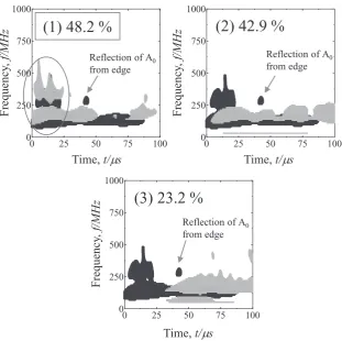
of 0-1 MHz. Interval of sampling frequency and time in wavelet contourmaps were 5 kHz and 200 ns, respectively. Thus, pixel size of 200 ×  512 was used to calculate agree-ment rate. Subsequently, the time-frequency coordinate of the high wavelet coefficient was extracted. Figure 10 shows the wavelet coefficient coordinate and the agreement rate be-tween experiment and simulations for each propagation an-gle. The agreement rate between the detected AE and the

0 simulation waveform was 48.2%, that between the de-tected AE and 45 simulation waveform was 42.9%, and that between the detected AE and 90 simulation waveform was 23.2%. That is, the 0 simulation waveform most suit-ably extracted the detected AE waveform features in the in-terval of 0–25 μs, and this AE was successfully classified as corresponding to θ =  0 . In this case, high wavelet coefficient area by an experiment was agree with that by the 0 simu-lation in the area from 15 μs to 20 μs in Fig. 10. It was esti-mated that A0 mode of lamb wave was contributed in high

agreement rate. However, reflected A0 wave was not

de-tected in the result of 0 simulation. It was implied that ac-curacy of simulation in reflection wave was not good enough. We need to consider the simulation accuracy on our future studies.

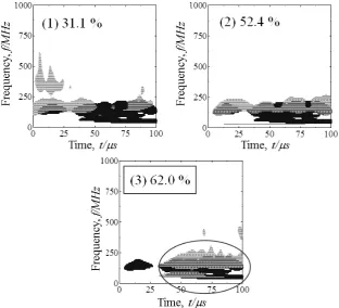
Next, we attempted to classify the AE detected in Test 3 at 282 s (Event Count: E.C 3-4). Figure 11 shows the AE waveform excited by the mode I fracture and the simulation waveforms convoluted with the sensor response for each propagation angle. As before, these waveforms were wave-let-transformed, and the time-frequency coordinate of the high wavelet coefficient was extracted. Figure 12 shows the wavelet coefficient coordinate and the agreement rate be-tween experiment and simulations for each propagation an-gle. The agreement rate between the detected AE and the 0

Fig. 11 Experimental waveform (E.C 3-4) and simulation waveforms (θ =  0 , 45 , and 90 ).

simulation waveform was 31.1%, that between the detected AE and the 45 simulation waveform was 52.4%, and that between the detected AE and the 90 simulation waveform was 62.0%. As a result, the 90 simulation waveform was considered to have satisfactorily extracted the detected AE waveform features after 30 μs, and this AE was successfully classified as corresponding to θ =  90 .

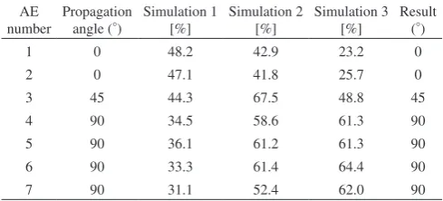
Table 1 lists the classification results of all AE signals via the AE pattern recognition method. All AE signals showed the highest agreement rate with the simulation waveforms of the actual propagation angles, thereby confirming successful classification; that is, the proposed AE pattern recognition method could classify the AE signals (with different propa-gation angles) excited by the mode I fracture of the glass fi-ber. From the table, we note that the agreement rates be-tween AE No. 5 and 6 and the 45 simulation waveform were close to the highest values. Further studies are needed in order to classify the AE signals more accurately and consistently.

5.  Conclusion

In this study, we developed an AE pattern recognition method based on simulated AE waveforms. The simulated AE waveform was a convolution of the simulated elastic wave calculated by the 3D FDTD method and the sensor re-sponse acquired with the use of the long bar method. AE signals with different propagation angles were subsequently classified, and the results indicated successful classification of all the AE signals. Therefore, we concluded that the pro-posed AE pattern recognition method could classify the AE signals with different propagation angles excited by mode I fracture of a glass fiber. In summary, we believe that this ap-proach can be utilized to estimate the fracture type from out-put AE waveforms.

REFERENCES

1) C. Hellier: Handbook of Nondestructive Evaluation, (McGraw-hill, New York, 2003), 10.1–10.39.

2) Y. Mizutani ed.: Practical Acoustic Emission Testing, (Springer Japan, Tokyo, 2016), pp. 5–12.

3) T. Kishi, M. Ohtsu and S. Yuyama: Acoustic Emission beyond the Millennium, (Elsevier Science, Amsterdam, 2000) pp.1–18.

4) N. Saito, M. Takemoto, H. Suzuki and K. Ono: Trans. of the J. Soc. for Comp. Mater. 26 (2000) 227–235 (In Japanese).

5) M.A. Hamstad, J. Gary and A. O Gallagher: JAE 17 (1999) 37–47. 6) K.S. Yee: IEEE Trans. Antennas Propag. AP-14 (1996) 302–307. 7) R. Kuwahara, H. Ojima, T. Matsuo and H. Cho: J. Solid Mech. Mater.

Eng. 7 (2013) 176–186.

8) K. Arakawa and T. Matsuo: Proceedings of the 2015 national Conference on acoustic emission, pp. 19–32 (In Japanese).

9) K. Ono, H. Cho and T. Matsuo: 29th European Conference on Acoustic Emission Testing, (2010) 426–434.

10) N. Saito, M. Takemoto, H. Suzuki and K. Ono: Transactions of the Japan Society for Composite Materials. 26 (2000) 179–186.

Table 1 Classification results of all acoustic emission (AE) signals.

AE number

Propagation angle ( )

Simulation 1 [%] Simulation 2 [%] Simulation 3 [%] Result ( )

1 0 48.2 42.9 23.2 0

2 0 47.1 41.8 25.7 0

3 45 44.3 67.5 48.8 45

4 90 34.5 58.6 61.3 90

5 90 36.1 61.2 61.3 90

6 90 33.3 61.4 64.4 90