Automatically Inferring Gender Associations from Language

Proceedings of the 2019 Conference on Empirical Methods in Natural Language Processing

5746

Automatically Inferring Gender Associations from Language

Serina Chang

Department of Computer Science Columbia University∗

[email protected]

Kathleen McKeown Department of Computer Science

Columbia University

[email protected]

Abstract

In this paper, we pose the question: do people talk about women and men in different ways? We introduce two datasets and a novel integra-tion of approaches for automatically inferring gender associations from language, discover-ing coherent word clusters, and labeldiscover-ing the clusters for the semantic concepts they repre-sent. The datasets allow us to compare how people write about women and men in two dif-ferent settings - one set draws from celebrity news and the other from student reviews of computer science professors. We demonstrate that there are large-scale differences in the ways that people talk about women and men and that these differences vary across domains. Human evaluations show that our methods sig-nificantly outperform strong baselines.

1 Introduction

It is well-established that gender bias exists in language – for example, we see evidence of this given the prevalence of sexism in abusive lan-guage datasets (Waseem and Hovy,2016;Jha and Mamidi,2017). However, these are extreme cases of gender norms in language, and only encompass a small proportion of speakers or texts.

Less studied in NLP is how gender norms man-ifest in everyday language – do people talk about women and men in different ways? These types of differences are far subtler than abusive language, but they can provide valuable insight into the roots of more extreme acts of discrimination. Subtle dif-ferences are difficult to observe because each case on its own could be attributed to circumstance, a passing comment or an accidental word. How-ever, at the level of hundreds of thousands of data points, these patterns, if they do exist, become un-deniable. Thus, in this work, we introduce new datasets and methods so that we can study subtle gender associations in language at the large-scale.

∗

Since writing this paper, Serina Chang has moved to the Department of Computer Science at Stanford University.

Our contributions include:

• Two datasets for studying language and gen-der, each consisting of over 300K sentences.

• Methods to infer gender-associated words and labeled clusters in any domain.

• Novel findings that demonstrate in both do-mains that people do talk about women and men in different ways.

Each contribution brings us closer to modeling how gender associations appear in everyday lan-guage. In the remainder of the paper, we present related work, our data collection, methods and findings, and human evaluations of our system.1

2 Related Work

The study of gender and language has a rich his-tory in social science. Its roots are often attributed to Robin Lakoff, who argued that language is fun-damental to gender inequality, “reflected in both the ways women are expected to speak, and the ways in which women are spoken of” (Lakoff,

1973). Prominent scholars following Lakoff have included Deborah Tannen (1990), Mary Bucholtz and Kira Hall (1995), Janet Holmes (2003), Pene-lope Eckert (2003), and Deborah Cameron (2008), along with many others.

In recent decades, the study of gender and language has also attracted computational re-searchers. Echoing Lakoff’s original claim, a pop-ular strand of computational work focuses on dif-ferences in how women and men talk, analyz-ing key lexical traits (Boulis and Ostendorf,2005;

Argamon et al., 2007; Bamman et al., 2014) and predicting a person’s gender from some text they have written (Rao et al., 2010; Jurgens et al.,

1_{Our datasets and code are available at}

2017). There is also research studying how people talktowomen and men (Voigt et al.,2018), as well as how people talk about women and men, typi-cally in specific domains such as sports journalism (Fu et al.,2016), fiction writing (Fast et al.,2016), movie scripts (Sap et al.,2017), and Wikipedia bi-ographies (Wagner et al.,2015,2016). Our work builds on this body by diving into two novel do-mains: celebrity news, which explores gender in pop culture, and student reviews of computer sci-ence (CS) professors, which examines gender in academia and, particularly, the historically male-dominated field of CS. Furthermore, many of these works rely on manually constructed lexi-cons or topics to pinpoint gendered language, but our methods automatically infer gender-associated words and labeled clusters, thus reducing supervi-sion and increasing the potential to discover sub-tleties in the data.

Modeling gender associations in language could also be instrumental to other NLP tasks. Abusive language is often founded in sexism (Waseem and Hovy,2016;Jha and Mamidi,2017), so models of gender associations could help to improve detec-tion in those cases. Gender bias also manifests in NLP pipelines: prior research has found that word embeddings preserve gender biases ( Boluk-basi et al.,2016;Caliskan et al.,2017;Garg et al.,

2018), and some have developed methods to re-duce this bias (Zhao et al.,2018,2019). Yet, the problem is far from solved; for example, Gonen and Goldberg 2019 showed that it is still possi-ble to recover gender bias from “de-biased” em-beddings. These findings further motivate our re-search, since before we can fully reduce gender bias in embeddings, we need to develop a deeper understanding of how gender permeates through language in the first place.

We also build on methods to cluster words in word embedding space and automatically label clusters. Clustering word embeddings has proven useful for discovering salient patterns in text cor-pora (Wilson et al., 2018;Demszky et al.,2019). Once clusters are derived, we would like them to be interpretable. Much research simply considers the top-nwords from each cluster, but this method can be subjective and time-consuming to interpret. Thus, there are efforts to design methods of auto-matic cluster labeling (Manning et al.,2008). We take a similar approach to Poostchi and Piccardi 2018, who leverage word embeddings and

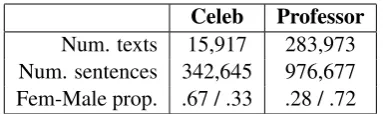
Word-Celeb Professor

Num. texts 15,917 283,973 Num. sentences 342,645 976,677 Fem-Male prop. .67 / .33 .28 / .72

Table 1: Summary statistics of our datasets.

Net during labeling, and we extend their method with additional techniques and evaluations.

3 Data Collection

Our first dataset contains articles from celebrity magazines People, UsWeekly, and E!News. We labeled each article for whether it was report-ing on men, women, or neither/unknown.2 To do this, we first extracted the article’s topic tags. Some of these tags referred to people, but oth-ers to non-people entities, such as “Gift Ideas” or “Health.” To distinguish between these types of tags, we queried each tag on Wikipedia and checked whether the top page result contained a “Born” entry in its infobox – if so, we concluded that the tag referred to a person.

Then, from the person’s Wikipedia page, we de-termined their gender by checking whether the in-troductory paragraphs of the page contained more male or female pronouns. This method was simple but effective, since pronouns in the introduction al-most always resolve to the subject of that page. In fact, on a sample of 80 tags that we manually an-notated, we found that comparing pronoun counts predicted gender with perfect accuracy. Finally, if an article tagged at least one woman and did not tag any men, we labeled the article as Female; in the opposite case, we labeled it as Male.

Our second dataset contains reviews from Rate-MyProfessors (RMP), an online platform where students can review their professors. We included all 5,604 U.S. schools on RMP, and collected all reviews for CS professors at those schools. We la-beled each review with the gender of the professor whom it was about, which we determined by com-paring the count of male versus female pronouns over all reviews for that professor. This method was again effective, because the reviews are

ex-2

pressly written about a certain professor, so the pronouns typically resolve to that professor.

In addition to extracting the text of the articles or reviews, for each dataset we also collected var-ious useful metadata. For the celebrity dataset, we recorded each article’s timestamp and the name of the author, if available. Storing author names creates the potential to examine the relationship between the gender of the author and the gender of the subject, such as asking if there are differ-ences between how women write about men and how men write about men. In this work, we did not yet pursue this direction because we wanted to begin with a simpler question of how gender is discussed: regardless of the gender of the au-thors, what is the content being put forth and con-sumed? Furthermore, we were unable to extract author gender in the professor dataset since the RMP reviews are anonymous. However, in future work, we may explore the influence of author gen-der in the celebrity dataset.

For the professor dataset, we captured metadata such as each review’s rating, which indicates how the student feels about the professor on a scale of AWFUL to AWESOME. This additional variable in our data creates the option in future work to factor in sentiment; for example, we could study whether there are differences in language used when criticizing a female versus a male professor.

4 Inferring Word-Level Associations

Our first goal was to discover words that are signif-icantly associated with men or women in a given domain. We employed an approach used by Bam-man et al. 2014 in their work to analyze differ-ences in how men and women write on Twitter.

4.1 Methods

First, to operationalize, we say that term iis as-sociated with gender j if, when discussing indi-viduals of gender j, i is used with unusual fre-quency – which we can check with statistical hy-pothesis tests. Let fi represent the likelihood of i appearing when discussing women or men. fi is unknown, but we can model the distribution of all possible fi using the corpus of texts that we have from the domain. We construct a gender-balanced version of the corpus by randomly un-dersampling the more prevalent gender until the proportions of each gender are equal. Assuming a non-informative prior distribution on fi, the

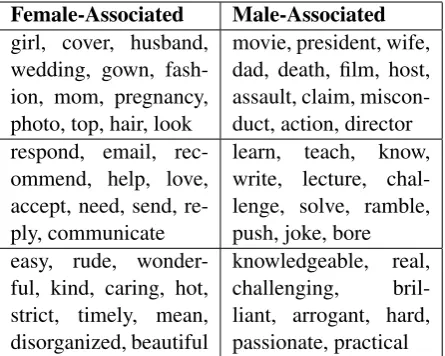
pos-Female-Associated Male-Associated

girl, cover, husband, wedding, gown, fash-ion, mom, pregnancy, photo, top, hair, look

movie, president, wife, dad, death, film, host, assault, claim, miscon-duct, action, director respond, email,

rec-ommend, help, love, accept, need, send, re-ply, communicate

learn, teach, know, write, lecture, chal-lenge, solve, ramble, push, joke, bore easy, rude,

wonder-ful, kind, caring, hot, strict, timely, mean, disorganized, beautiful

knowledgeable, real, challenging, bril-liant, arrogant, hard, passionate, practical

Table 2: Top: Sample from the top-25 most gender-associatednounsin the celebrity domain.Middle: pro-fessor domain, sample from top-25 verbs. Bottom: professor domain, sample from top-25adjectives. All associations listed arep≤0.05, with Bonferroni cor-rection. See Appendix for all top-25 nouns, verbs, and adjectives for both genders in both domains.

terior distribution is Beta(ki,N−ki), wherekiis the count ofi in the gender-balanced corpus and N is the total count of words in that corpus.

As Bamman et al. 2014 discuss, “the distribu-tion of the gender-specific counts can be described by an integral over all possible fi. This inte-gral defines the Beta-Binomial distribution ( Gel-man et al.,2004), and has a closed form solution.” We say that termiis significantly associated with genderjif the cumulative distribution atkij (the count ofiin thejportion of the gender-balanced corpus) isp ≤ 0.05. As in the original work, we apply the Bonferroni correction (Dunn,1961) for multiple comparisons because we are computing statistical tests for thousands of hypotheses.

4.2 Findings

asked questions about their careers and creative processes (as an example, seeSelby 2014).

Table2also includes some of the most gender-associated verbs and adjectives from the professor domain. Female CS professors seem to be praised for being communicative and personal with stu-dents (“respond,” “communicate,” “kind,” “car-ing”), while male CS professors are recognized for being knowledgeable and challenging the stu-dents (“teach,”, “challenge,” “brilliant,” “practi-cal”). These trends are well-supported by so-cial science literature, which has found that fe-male teachers are praised for “personalizing” in-struction and interacting extensively with students, while male teachers are praised for using “teacher as expert” styles that showcase mastery of material (Statham et al.,1991).

These findings establish that there are clear dif-ferences in how people talk about women and men – even with Bonferroni correction, there are still over 500 significantly gender-associated nouns, verbs, and adjectives in the celebrity domain and over 200 in the professor domain. Furthermore, the results in both domains align with prior stud-ies and real world trends, which validates that our methods can capture meaningful patterns and innovatively provide evidence at the large-scale. This analysis also hints that it can be helpful to abstract from words to topics to recognize higher-level patterns of gender associations, which moti-vates our next section on clustering.

5 Clustering & Cluster Labeling

With word-level associations in hand, our next goals were to discover coherent clusters among the words and to automatically label those clusters.

5.1 Methods

First, we trained domain-specific word embed-dings using the Word2Vec (Mikolov et al.,2013) CBOW model (w ∈ R100). Then, we used k-means clustering to cluster the embeddings of the gender-associated words. Since k-means may con-verge at local optima, we ran the algorithm 50 times and kept the model with the lowest sum of squared errors.

To automatically label the clusters, we com-bined the grounded knowledge of WordNet (Miller, 1995) and context-sensitive strengths of domain-specific word embeddings. Our algorithm is similar to Poostchi and Piccardi 2018’s

ap-proach, but we extend their method by introduc-ing domain-specific word embeddintroduc-ings for cluster-ing as well as a new technique for sense disam-biguation. Given a cluster, our algorithm proceeds with the following three steps:

1. Sense disambiguation: The goal is to as-sign each cluster word to one of its WordNet synsets; letSrepresent the collection of cho-sen synsets. We know that these words have been clustered in domain-specific embedding space, which means that in the context of the domain, these words are very close semanti-cally. Thus, we chooseS∗that minimizes the total distance between its synsets.

2. Candidate label generation: In this step, we generateL, the set of possible cluster labels. Our approach is simple: we take the union of all hypernyms of the synsets inS∗.

3. Candidate label ranking: Here, we rank the synsets inL. We want labels that are as close to all of the synsets in S∗ as possible; thus, we score the candidate labels by the sum of their distances to each synset in S∗ and we rank them from least to most distance.

In steps 1 and 3, we use WordNet pathwise dis-tance, but we encourage the exploration of other distance representations as well.

5.2 Findings

Table3displays a sample of our results – we find that the clusters are coherent in context and the la-bels seem reasonable. In the next section, we dis-cuss human evaluations that we conducted to more rigorously evaluate the output, but first we discuss the value of these methods toward analysis.

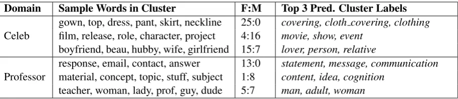
Domain Sample Words in Cluster F:M Top 3 Pred. Cluster Labels

Celeb

gown, top, dress, pant, skirt, neckline 25:0 covering, cloth covering, clothing film, release, role, character, project 4:16 movie, show, event

boyfriend, beau, hubby, wife, girlfriend 15:7 lover, person, relative

Professor

response, email, contact, answer 13:0 statement, message, communication material, concept, topic, stuff, subject 1:8 content, idea, cognition

teacher, woman, lady, prof, guy, dude 5:7 man, adult, woman

Table 3: Sample of our clusters and predicted cluster labels. We include in the Appendix a more comprehensive table of our results.F:Mrefers to the ratio of female-associated to male-associated words in the cluster.

pulling out the patterns that we believed we saw at the word-level, but could not formally validate.

The clusters we mentioned so far all lean heav-ily toward one gender association or the other, but some clusters are interesting precisely be-cause they do not lean heavily – this allows us to see where semantic groupings do not align exactly with gender association. For example, in the celebrity domain, there is a cluster la-beled lover that has a mix of female-associated words (“boyfriend,” “beau,” “hubby”) and male-associated words (“wife,” “girlfriend”). Jointly leveraging cluster labels and gender associations allows us to see that in the semantic context of hav-ing a lover, women are typically associated with male figures and men with female figures, which reflects heteronormativity in society.

6 Human Evaluations

To test our clusters, we employed the Word In-trusiontask (Chang et al.,2009). We present the annotator with five words – four drawn from one cluster and one drawn randomly from the domain vocabulary – and we ask them to pick out the in-truder. The intuition is that if the cluster is co-herent, then an observer should be able to identify the out-of-cluster word as the intruder. For both domains, we report results on all clusters and on the top 8, ranked by ascending normalized sum of squared errors, which can be seen as a prediction of coherence. In the celebrity domain, annotators identified the out-of-cluster word 73% of the time in the top-8 and 53% overall. In the professor do-main, annotators identified it 60% of the time in the top-8 and 49% overall. As expected, top-8 per-formance in both domains does considerably bet-ter than overall, but at all levels the precision is significantly above the random baseline of 20%.

To test cluster labels, we present the annota-tor with a label and a word, and we ask them

whether the word falls under the concept. The concept is a potential cluster label and the word is either a word from that cluster or drawn ran-domly from the domain vocabulary. For a good label, the rate at which in-cluster words fall un-der the label should be much higher than the rate at which out-of-cluster words fall under. In our experiments, we tested the top 4 predicted labels and the centroid of the cluster as a strong base-line label. The centroid achieved an in-cluster rate of .60 and out-of-cluster rate of .18 (difference of .42). Our best performing predicted label achieved an in-cluster rate of .65 and an out-of-cluster rate of .04 (difference of .61), thus outperforming the centroid on both rates and increasing the gap be-tween rates by nearly 20 points. In the Appendix, we include more detailed results on both tasks.

7 Conclusion

References

Shlomo Argamon, Moshe Koppel, James Pennebaker, and Jonathan Schler. 2007. Mining the blogosphere: age, gender, and the varieties of self-expression.

First Monday, 12(9).

David Bamman, Jacob Eisenstein, and Tyler Schnoe-belen. 2014. Gender identity and lexical variation in social media. Journal of Sociolinguistics, 18(2).

Tolga Bolukbasi, Kai-Wei Chang, James Zou, Venkatesh Saligrama, and Adam Kalai. 2016. Man is to computer programmer as woman is to home-maker? debiasing word embeddings. InNeurIPS.

Constantinos Boulis and Mari Ostendorf. 2005. A quantitative analysis of lexical differences between genders in telephone conversations. InACL.

Mary Bucholtz and Kira Hall. 1995. Gender articu-lated: language and the socially constructed self. Routledge.

Aylin Caliskan, Joanna J. Bryson, and Arvind Narayanan. 2017. Semantics derived automatically from language corpora contain human-like biases.

Science, 356(6334).

Deborah Cameron. 2008. The myth of mars and venus: do men and women really speak different lan-guages? Oxford University Press.

Jonathan Chang, Sean Gerrish, Chong Wang, Jordan L. Boyd-Graber, and David M. Blei. 2009. Reading tea leaves: how humans interpret topic models. In

NeurIPS.

Dorottya Demszky, Nikhil Garg, Rob Voigt, James Zou, Matthew Gentzkow, Jesse Shapiro, and Dan Ju-rafsky. 2019. Analyzing polarization in social me-dia: method and application to tweets on 21 mass shootings. InNAACL.

Olive Jean Dunn. 1961. Multiple comparisons among means. Journal of the American Statistical Associa-tion, 56(293).

Penelope Eckert and Sally McConnell-Ginet. 2003.

Language and gender. Cambridge University Press.

Ethan Fast, Tina Vachovsky, and Michael Bernstein. 2016. Shirtless and dangerous: quantifying linguis-tic signals of gender bias in an online fiction writing community. InICWSM.

Liye Fu, Cristian Danescu-Niculescu-Mizil, and Lil-lian Lee. 2016. Tie-breaker: using language mod-els to quantify gender bias in sports journalism. In

IJCAI Workshop on NLP Meets Journalism.

Nikhil Garg, Londa Schiebinger, Dan Jurafsky, and James Zou. 2018. Word embeddings quantify 100 years of gender and ethnic stereotypes.Proceedings of the National Academy of Sciences, 155(16).

Andrew Gelman, John B. Carlin, Hal S. Stern, and Donald B. Rubin. 2004. Bayesian data analysis. CRC Press/Chapman Hall.

Hila Gonen and Yoav Goldberg. 2019. Lipstick on a pig: debiasing methods cover up systematic gender biases in word embeddings but do not remove them. InNAACL-HLT.

Janet Holmes and Miriam Meyerhoff. 2003. The hand-book of language and gender. Blackwell Publish-ing.

Akshita Jha and Radhika Mamidi. 2017. When does a compliment become sexist? analysis and classifi-cation of ambivalent sexism using twitter data. In

ACL Workshop on NLP and Computational Social Science.

David Jurgens, Yulia Tsvetkov, and Dan Jurafsky. 2017. Writer profiling without the writers text. In

SocInfo.

Robin Lakoff. 1973. Language and woman’s place.

Language in Society, 2(1).

Christopher D. Manning, Prabhakar Raghavan, and Hinrich Schutze. 2008. Introduction to information retrieval. Cambridge University Press.

Tomas Mikolov, Kai Chen, Gregory Corrado, and Jef-frey Dean. 2013. Efficient estimation of word repre-sentations in vector space. InICLR Workshop.

George A. Miller. 1995. Wordnet: a lexical database for english. Communications of the ACM, 38(11).

Hanieh Poostchi and Massimo Piccardi. 2018. Cluster labeling by word embeddings and wordnet’s hyper-nymy. InAustralasian Language Technology Asso-ciation Workshop.

Delip Rao, David Yarowsky, Abhishek Shreevats, and Manaswi Gupta. 2010. Classifying latent user at-tributes in twitter. InSMUC.

Maarten Sap, Marcella Cindy Prasetio, Ari Holtzman, Hannah Rashkin, and Yejin Choi. 2017. Connota-tion frames of power and agency in modern films. InEMNLP.

Jenn Selby. 2014. Cate blanchett calls out red carpet sexism: ‘do you do this to the guys?’. In Indepen-dent.

Anna Statham, Laurel Richardson, and Judith A. Cook. 1991.Gender and university teaching: a negotiated difference. SUNY Press.

Deborah Tannen. 1990.You just dont understand: men and women in conversation. Ballantine Books.

Claudia Wagner, David Garcia, Mohsen Jadidi, and Markus Strohmaier. 2015. It’s a man’s wikipedia? assessing gender inequality in an online encyclope-dia. InICWSM.

Claudia Wagner, Eduardo Graells-Garrido, David Gar-cia, and Filippo Menczer. 2016. Women through the glass ceiling: gender asymmetries in wikipedia.

EPJ Data Sci, 5(5).

Zeerak Waseem and Dirk Hovy. 2016. Hateful sym-bols or hateful people? predictive features for hate speech detection on twitter. InNAACL-HLT.

Steven Wilson, Yiting Shen, and Rada Mihalcea. 2018. Building and validating hierarchical lexicons with a case study on personal values. InSocInfo.

Jieyu Zhao, Tianlu Wang, Mark Yatskar, Ryan Cot-terell, Vicente Ordonez, and Kai-Wei Chang. 2019. Gender bias in contextualized word embeddings. In

NAACL-HLT.