Applying EM Algorithm for Segmentation of
Textured Images
Dr. K Revathy, Dept. of Computer Science, University of Kerala, India Roshni V. S., ER&DCI Institute of Technology, CDAC-T, India
Abstract— Texture analysis plays an increasingly important role in computer vision. Since the textural properties of images appear to carry useful information for discrimination purposes, it is important to develop significant features for texture. Various texture feature extraction methods include those based on gray-level values, transforms, auto correlation etc. We have chosen the Gray Level Co occurrence Matrix (GLCM) method for extraction of feature values. Image segmentation is another important problem and occurs frequently in many image processing applications. Although, a number of algorithms exist for this purpose, methods that use the Expectation-Maximization (EM) algorithm are gaining a growing interest. The main feature of this algorithm is that it is capable of estimating the parameters of mixture distribution. This paper presents a novel unsupervised segmentation method based on EM algorithm in which the analysis is applied on vector data rather than the gray level value.
Index Terms—Texture, Segmentation, GLCM, EM, Bayes
INTRODUCTION
Image segmentation is a fundamental task in machine vision and occurs very frequently in many image-processing applications. Texture based segmentation provides an important cue to the recognition of objects. Texture is one of the visual features playing an important role in scene analysis. Intuitively, it is related to patterned variations of intensity across an image. Texture segmentation in general is composed of two steps, namely, the extraction of texture based features and secondly the grouping of these features.
There are a number of methods for texture feature extraction. These methods can be classified into feature-based methods, model-based methods, and structure-based methods. Structure-based methods partition images under the assumption that the textures in the image have detectable primitive elements, arranged according to placement rules. In feature-based methods, regions with relatively constant texture characteristics are sought. Model-based methods hypothesize underlying processes for textures and segments using certain parameters of these processes. Model based methods can be considered as a subclass of feature-based methods since model parameters are used as texture features.
This paper describes an unsupervised segmentation technique with maximum-likelihood parameter estimation
problem for parameter estimation and the Expectation-Maximization problem for its solution. The main feature of this algorithm is that it is capable of estimating the parameters of mixed distribution. Texture measures are derived using the gray-level co occurrence matrices.The EM algorithm is applied to estimate the mean and variance of features for every texture in the image. At last a Bayesian classification rule is applied to attribute a label for each pixel by defining a likelihood function, which computes the probability for a given pixel as belonging to a given class.
Texture analysis has been used in a range of studies for recognizing synthetic and natural textures. It is very useful in the analysis of aerial images, biomedical images and seismic images as well as the automation of industrial applications.
I. IMAGE TEXTURE
Texture is an important property of many types of images. While there isn’t a universally agreed definition of what a texture is, features of a texture include roughness, granulation and regularity. Visual texture contains variations of intensities, which form certain repeated patterns. Those patterns can be caused by physical surface properties, such as roughness, or they could result from reflectance differences, such as the color on a surface. Texture is an important part of the visual world of animals and men and their visual systems successfully detect, discriminate and segment texture.
A class of simple image properties that can be used for texture analysis are the first-order statistics of local property values, i.e., the mean, variance, etc. In particular, a class of local properties based on absolute differences between pairs of gray levels or average gray levels has performed well; Usually different kinds of measures are derived from difference histograms, such as contrast, angular second moment, entropy, mean, and inverse difference moment.
Figure 1: Images consisting of different textured regions
image to obtain a boundary map. Texture classification deals with the recognition of image regions using texture properties. Each region in an image is assigned a texture class. The goal of texture synthesis is to extract three-dimensional information from texture properties.
II. IMAGE SEGMENTATION
A central problem, called segmentation, is to distinguish objects from background. An image consists of a number of natural objects defined by distinct regions. The image background in itself is a distinct region. These regions are defined by their boundaries that separate them from other regions. Image segmentation aims at identifying these boundaries and as to which pixel comes from which region. The segmentation problem can be informally described as the task of partitioning an image into homogeneous regions. For textured images one of the main conceptual difficulties is the definition of a homogeneity measure in mathematical terms. A texture method is a process that can be applied to a pixel of a given image in order to generate a measure (feature) related to the texture pattern to which that pixel and its neighbors belong. The performance of the different families of texture methods basically depends on the type of processing they apply, the neighborhood of pixels over which they are evaluated (evaluation window) and the texture content.
Texture methods used can be categorized as: statistical, geometrical, structural, model-based and signal processing features [1]. Van Gool et al. [2] and Reed and Buf [3] present a detailed survey of the various texture methods used in image analysis studies. Randen and Husoy [4] conclude that most studies deal with statistical, model-based and signal processing techniques. Weszka et al. [5] compared the Fourier spectrum; second order gray level statistics, co-occurrence statistics and gray level run length statistics and found the co-occurrence were the best. Similarly, Ohanian and Dubes [6] compare Markov Random Field parameters, multi-channel filtering features, fractal based features and co-occurrence matrices features, and the co-occurrence method performed the best. The same conclusion was also drawn by Conners and Harlow [7] when comparing run-length difference, gray level difference density and power spectrum. Buf et al. [8] however report that several texture features have roughly the same performance when evaluating co-occurrence features, fractal dimension, transform and filter bank features, number of gray level extrema per unit area and curvilinear integration features. Compared to filtering features [9], co occurrence based features were found better as reported by Strand and Taxt [10], however, some other studies have supported exactly the
reverse. Pichler et al. [11] compare wavelet transforms with adaptive Gabor filtering feature extraction and report superior results using Gabor technique. However, the computational requirements are much larger than needed for wavelet transform, and in certain applications accuracy may be compromised for a faster algorithm. Ojala et al. [12] compared a range of texture methods using nearest neighbour classifiers including gray level difference method, Law's measures, center-symmetric covariance measures and local binary patterns applying them to Brodatz images. The best performance was achieved for the gray level difference method. Law's measures are criticized for not being rotationally invariant, for which reason other methods performed better.
III. PROPOSED METHOD
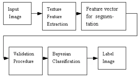
This section describes in detail the proposed technique for feature extraction and classification . The overall block diagram of texture feature extraction and classification and hence segmentation of the input image is presented in Figure 2. The proposed technique is divided into three stages. Stage 1 deals with the quantization and feature extraction from the texture images, stage 2 deals with the estimation of the Gaussian parameters by applying the EM algorithm and finally stage 3 implements the labeling process and thereby the segmentation of the texture regions.
A. Feature Extraction
The feature extraction algorithms analyze the spatial distribution of pixels in grey scale images. The different methods capture how coarse or fine a texture is. The textural character of an image depends on the spatial size of texture primitives. Large primitives give rise to coarse texture and small primitives fine texture. To model these characteristics, spatial methods are found to be superior to spectral methods. The most commonly used texture measures are those derived from the Grey Level Co-occurrence Matrix (GLCM). Haralick suggested the use of grey level co-occurrence matrices (GLCM) to extract second order statistics from an image. GLCMs have been used very successfully for texture segmentation.
The GLCM is a tabulation of how often different combinations of pixel brightness values (grey levels) occur in an image.
[image:2.612.320.543.577.701.2]Haralick defined the GLCM as a matrix of frequencies at which two pixels, separated by a certain vector, occur in the image. The distribution in the matrix will depend on the angular and distance relationship between pixels. Varying the vector used allows the capturing of different texture characteristics. Once the GLCM has been created, various features can be computed from it. These have been classified into four groups: visual texture characteristics, statistics, information theory and information measures of correlation.
To reduce the computational time required for extracting features for 256 pixel values the input image is quantized before applying the feature extraction process. Quantization can be done either to the pixel values or to the spatial coordinates. Operation on pixel values is referred to as gray-level reduction and operating on the spatial coordinates is called spatial reduction.
Texture feature extraction is performed on the quantized image by using Gray level co-occurrence matrix (GLCM) method, one of the most known texture analysis method which estimates image properties related to second-order statistics. A GLCM or SGLD matrix is the joint probability occurrence of gray levels i and j for two pixels with a defined spatial relationship in an image. The spatial relationship is defined in terms of distance d and angle θ. If the texture is coarse and distance d is small compared to the size of the texture elements, the pairs of points at distance d should have similar gray levels. Conversely, for a fine texture, if distance d is comparable to the texture size, then the gray levels of points separated by distance d should often be quite different, so that the values in the SGLD matrix should be spread out relatively uniformly. From SGLD matrices, a variety of features may be extracted. From each matrix, 14 statistical measures are extracted including: angular second moment, contrast, correlation, variance, inverse different moment, sum average, sum variance, sum entropy, difference variance, difference entropy, information measure of correlation I, information measure of correlation II, and maximal correlation coefficient. The measurements average the feature values in all four directions. The results may be combined by averaging the GLCM for each angle before calculating the features or by averaging the features calculated for each GLCM. To reduce the computational complexity, only some of the features were selected. In our experiments gray level co occurrence matrices were calculated for each pixel using a neighborhood of size 8 x 8 at angles of 0, 45, 90, 135 etc.
Algorithm for creating a symmetrical normalized GLCM 1. Create a framework matrix
2. Decide on the spatial relation between the reference and neighbour pixel
3. Count the occurrences and fill in the framework matrix 4. Add the matrix to its transpose to make it symmetrical 5. Normalize the matrix to turn it into probabilities
6. Change the value of angle and offset to get matrices in the other directions.
B. Features calculated from a normalized GLCM based on textures
N-1 i,j i,j=0
Contrast= P (
∑
i
−
j
)
(1)N-1 i,j i,j=0
Dissimilarity= P |
∑
i
−
j
|
(2)
i,j i,j
2 N-1
i,j=0
P
Homogeneity=
P
1+(i-j)
∑
(3)N-1 2 i,j i,j=0
Energy
∑
(P )
(4)N-1
i,j , i,j=0
Entropy =
∑
P ( ln
−
P
i j)
(5)Mean:
1 ( , ) , 0
(
)
N
i i
i j
i P
µ
−=
=
∑
j)
j 1
( , ) , 0
(
N
j i
i j
j P
µ
−=
=
∑
(6)Variance:
N-1
2 2
i ,
i,j=0
= (
P i
i j i)
σ
∑
−
µ
(7)N-1
2 2
j ,
i,j=0
= (
P
i jj
j)
σ
∑
−
µ
(8)Correlation = N-1
, 2 2
i,j=0
(
i)(
j)
i j
i j
i
j
P
µ
µ
σ σ
⎡
−
−
⎤
⎢
⎥
⎢
⎥
⎣
⎦
∑
(9)We had calculated the features from the co occurrence matrices obtained . The average of the features for each case gives the feature value for the particular case. Typical values obtained for one of the test images is shown in Table 1.
C. Maximum Likelihood Estimation
Figure 3: Maximum-likelihood estimation and relative-frequency estimation
We also have a data set of size N, supposedly drawn from this distribution, i.e., X = {x 1,………., x N}. That is, we assume
that these data vectors are independent and identically distributed with distribution p. Therefore, the resulting density for the samples is
1
( / )
N( | )
i( | )
i
p X
θ
p x
θ
L
==
∏
=
θ
X
θ
This function L (θ | X) is called the likelihood of the parameters given the data, or just the likelihood function. The likelihood is thought of as a function of the parameter θ where the data Xis fixed. In the maximum likelihood problem, our goal is to find the θ that maximizes L. That is, we wish to find
θ * where
*
arg max
L
( | )
X
θ
θ
=
θ
D. Expectation-Maximization (EM) algorithm
The EM algorithm is a general method of finding the maximum-likelihood estimate of the parameters of an underlying distribution from a given data set when the data is incomplete or has missing values.
There are two main applications of the EM algorithm. The first occurs when the data indeed has missing values, due to problems with or limitations of the observation process. The second occurs when optimizing the likelihood function is analytically intractable but when the likelihood function can be simplified by assuming the existence of and values for additional but missing (or hidden) parameters. The latter application is more common in the computational pattern recognition community [13,14].
Let X be the observed data generated by some distribution and suppose a complete data set exists Z = ( X,Y ) . We also have a joint density function
p ( z | θ ) = p ( x ,y | θ ) = p ( y | x , θ ) p(x | θ )
We can define a likelihood function L ( θ | Z ) = L ( θ | X,Y ) = p ( X , Y | θ ) , called the complete data likelihood. The original likelihood L (θ | X) is referred to as the incomplete data likelihood function.
The EM algorithm first finds the expected value of the complete data log likelihood log p ( X , Y | θ ) with respect to
the unknown data Y given the observed data X and the current parameter estimates. That is, we define:
(i-1) ( 1)
Q( ,
θ θ
)
=
E
[log ( , | ) | ,
p X Y
θ
X
θ
i−]
where θ (i – 1) is the current parameter estimate used to
evaluate the expectation and θ is the new parameter optimized to increase Q. The evaluation of this expectation is called the E-step of the algorithm.
The second step of the EM algorithm is to maximize the expectation computed in the first step.
(i)
arg max
Q
( ,
( 1)i)
θ
θ
=
θ
−These two steps are repeated as necessary. Each iteration is guaranteed to increase the log- likelihood and the algorithm is guaranteed to converge to a local maximum of the likelihood function.
In the case of a Gaussian distribution, the iterative EM algorithm for density function parameter estimation is given by:
(
)
1
\
( )
( \ ( ))
k k
j j i j k
j i L
k
j i l i
i
f x
x
f x
k
π
θ
ω
π
θ
=
=
∑
1
1
1/
N( )
k k
j j
i
N
x
π
+ω
=
=
∑
i1 ( 1) ( )
1
1
( )( )
N
k k
j k j
i j
i i
x x
N
µ
ω
π
+
+ =
=
∑
2 ( 1) ( ) ( 1) 2
( 1) 1
1
[( ) ]
k N k( )[
]
j k j i i
i j
x x
N
σ
ω
π
+ +
+ =
=
∑
−
kj
µ
where
ω
jk
( )
x
i is an intermediate function. [image:4.612.319.517.565.709.2]A validation procedure is also added to aid the EM process. The procedure is terminated if the difference between the estimated parameters of two consecutive EM steps is inferior to a fixed threshold ε.
Figure 5: Procedure of the EM algorithm
Algorithm
1. Initialize the value for the mixture parameters 2. Calculate the intermediate function for the
given set of initial values
3. Calculate the new mixture parameters by using
the intermediate function and the previous mixture values.
4. Continue the calculation until the threshold or
validation condition is met.
5. Repeat for each class of texture in the image.
E. Bayesian Classification
Classification is a basic task in data analysis and pattern recognition that requires the construction of a classifier that is a function that assigns a class label to instances described by a set of attributes. The classifier takes an unlabeled example and assigns it to a class. Numerous approaches to this problem are based on various functional representations such as decision trees, decision lists, neural networks, decision graphs, and rules. One of the most effective classifiers, in the sense that its predictive performance is competitive with state-of-the-art classifiers, is the Bayesian classifiers.
This classifier learns from training data the conditional probability of each attribute Ai given the class label C.
Classification is then done by applying Bayes rule to compute the probability of C given the particular instance of A 1
…………..An , and then predicting the class with the highest
posterior probability. So Bayesian classification and decision making is based on probability theory and the principle of choosing the most probable or the lowest risk (expected cost) option. Assume that there is a classification task to classify feature vectors (samples) to K different classes. A feature vector is denoted as x = [x1, x2,…..,xD]T where D is the
dimension of a vector. The probability that a feature vector x belongs to class
ω
k isP
(
ω
k|
x
)
. The classification of thevector is done according to posterior probabilities or decision risks calculated from the probabilities.
The posterior probabilities can be computed with the Bayes formula
( |
) ( )
(
| )
( )
k k
k
P x
P
P
x
P x
ω
ω
ω
=
where
P
(
x
|
ω
k)
is the probability density function of class kω
in the feature space andP
(
ω
k)
is the apriori probability,which tells the probability of the class before measuring any features. If prior probabilities are not actually known, they can be estimated by the class proportions in the training set. The divisor
1
( )
K( | ) ( )
i ii
P x
P x
ω
P
ω
==
∑
is merely a scaling factor to assure that posterior probabilities are really probabilities, i.e., their sum is one.
After estimating the Gaussian parameters that correspond to each region a labelisation process is required in order to attribute a label to each pixel. This is carried out by using the Bayesian classification method.
Algorithm
1. Calculate the probability for each pixel value in
the feature vector
2. Normalize the value by multiplying weight and
dividing by the sum total
3. Find the product of the probability matrix for
different texture features
4. Calculate the probability for each pixel to
belong to a particular class
5. Assign label to each class. IV. RESULTS
The method has been tested on a number of 256x256 grey level images from the Brodatz textures . Using GLCM method with an offset of 1 and for 4 different angles the different texture features were extracted. The parameters of the Gaussian mixture model were calculated for each texture in the image using EM algorithm. A likelihood function is calculated which gives the probability of a pixel as belonging to a particular class which forms the basis of labeling of the pixel.
For the test image taken, the amount of local variations in the image is considerable as indicated by the high contrast value obtained. It also indicates that most elements do not lie on the diagonal of the GLCM. The difference of each element from other elements of the co-occurrence matrix is indicated by the dissimilarity feature. Homogeneity is measure for uniformity of
TABLE I: TYPICAL VALUES FOR THE TEXTURE FEATURES OBTAINED FOR THE
SAMPLE TEST IMAGE
[image:5.612.363.518.633.721.2]
Figure 6.1 Test Image Figure 6.2 Dissimilarity feature
Figure 6.3 Energy feature Figure 6.4Homogeneity feature
Figure 6.5 Entropy feature Figure 6.6 Segmented Image
co-occurrence matrix, and if most elements lie on the main diagonal, its value will be large, compared to other case. Energy is the measure of the textural uniformity of the image. It reaches a high value when gray level distribution has either a constant or a periodic form. Entropy measures randomness and it will be very large when all elements of the co- occurrence matrix are same. When the image is not texturally uniform, the GLCM elements will have small values and therefore entropy is large. The above values can be represented pictorially as shown above.
The segmented image shows reasonably good accuracy. Accuracy can be improved by using additional features from the GLCM.
REFERENCES
[1] M. Tuceyran and A.K. Jain, "Texture analysis", Handbook of Pattern Recognition and Computer Vision, C.H. Chen, L.F. Pau and P.S.P. Wang (Eds.), chapter 2, pp. 235-276, World Scientific, Singapore, 1993. [2] L. vanGool, P. Dewaele and A. Oosterlinck, "Texture analysis",
Computer Vision, Graphics and Image Processing, vol. 29, pp. 336-357, 1985.
[3] T. R. Reed and J.M.H. Buf, "A review of recent texture segmentation and feature extraction techniques", Computer Vision, Image Processing and Graphics, vol. 57, no. 3, pp. 359-372, 1993.
[4] T. Randen and J.H. Husoy, "Filtering for texture classification: A comparative study", IEEE Transactions on Pattern Analysis and Machine Intelligence, vol. 21, no. 4, pp. 291
[5] J.S. Weszka, C. R. Dyer and A. Rosenfeld, "A comparative study of texture measures for terrain classification", IEEE Transactions on Systems, man and Cybernetics, vol. 6, pp. 269-285, 1976.
[6] P.P. Ohanian and R.C. Dubes, "Performance evaluation for four class of texture features", Pattern Recognition, vol. 25, no. 8, pp. 819-833, 1992.
[7] R.W. Conners and C.A. Harlow, "A theoretical comparison of texture algorithms", IEEE Transactions on Pattern Analysis and Machine Intelligence, vol. 2, no. 3, pp. 204-222, 1980.
[8] J.M.H. Buf, M. Kardan and M. Spann, "Texture feature performance for image segmentation", Pattern Recognition, vol. 23, no. 3/4, pp. 291-309, 1990.
[9] T. Randen and J.H. Husoy, "Filtering for texture classification: A comparative study", IEEE Transactions on Pattern Analysis and Machine Intelligence, vol. 21, no. 4, pp. 291-310, 1999.
[10] J. Strand and T. Taxt, "Local frequency features for texture classification", Pattern Recognition, vol. 27, no. 10, pp. 1397-1406, 1994. [11] O. Pichler, A. Teuner and B.J. Hosticka, "A comparison of texture feature extraction using adaptive Gabor filter, pyramidal and tree structured wavelet transforms", Pattern Recognition, vol. 29, no. 5, pp. 733-742, 1996.
[12] T. Ojala, M. Pietikainen, "A comparative study of texture measures with classification based on feature distributions, Pattern Recognition, vol. 29, no. 1, pp. 51-59, 1996.