Sentiment analysis under temporal shift

Proceedings of the 9th Workshop on Computational Approaches to Subjectivity, Sentiment and Social Media Analysis, pages 65–71 65

Sentiment analysis under temporal shift

Jan Lukes and Anders Søgaard

Dpt. of Computer Science University of Copenhagen Copenhagen, Denmark [email protected]

Abstract

Sentiment analysis models often rely on training data that is several years old. In this paper, we show that lexical features change polarity over time, leading to de-grading performance. This effect is par-ticularly strong in sparse models relying only on highly predictive features. Using predictive feature selection, we are able to significantly improve the accuracy of such models over time.

1 Introduction

Sentiment analysis models often rely on data that is several years old. Such data, e.g., product reviews, continuously undergo shifts, leading to changes in term frequency, for example. We also observe the emergence of novel expressions, as well as the amelioration and pejoration of words (Cook and Stevenson, 2010). Such changes are typically studied over decades or centuries; how-ever, we hypothesize that change is continuous, and small changes can be detected over shorter time spans (years), and that their cumulation can influence the quality of sentiment analysis mod-els. In this paper, we analyze temporal polarity changes of individual features using product re-views data. Additionally, we show that predictive feature selection, trying to counteract shifts in po-larity, significantly improves model accuracy over time.

Contributions First, we show deterioration of sentiment analysis model performance over time. We propose rank-based metrics for detecting po-larity shifts and identify several examples of lexi-cal features that exhibit temporal drift in our data. Finally, we use our findings to design a predictive feature selection scheme, based on expected polar-ity changes, and show that models using predictive

Sample positive review:

”Grand daughters really like this movie. Good clean movie for all ages. Would recommend for

everyone. Good horse movie for girls.”

Sample negative review:

”Not what I expected. Very cheap and chintzy looking for the price. Certainly did not look like a

wallet. Very disappointed in the quality.”

Figure 1: Examples of reviews

feature selection perform significantly better than models that simply rely on the most predictive fea-tures across the training data without estimating temporal shifts.

Training data Model accuracy

Runs 1 2 3 Mean

2001-2004 0.858 0.855 0.863 0.859 2008-2011 0.877 0.873 0.878 0.877

Table 1: Classifier accuracy deterioration when using older and newer training sets. Models were trained using random independent data subsets from periods 2001-2004 or 2008-2011 and tested using random independent subsets from 2012-2014. Subset size:K= 40,000with 80/20 split.

2 Sentiment analysis models get worse over time

One way we may observe polarity shifts over time is when we see models trained on older data per-form worse than models trained on more recent data. Or, equivalently, by seeing performance degradations over time.

will use in our experiments, is a collection of user product reviews and meta-data crawled from Amazon.com, consisting of 82 million reviews and spanning May 1996 until July 2014 (He and McAuley,2016;McAuley et al.,2015). Previous work already preprocessed the dataset, removing duplicates and boiler plates. We sample large sub-samples of reviews per year from the original data set (K = 40000). Only years 2001 to 2014 were used in this project, as the samples from earlier years were of insufficient size.

Following previous work (Blitzer et al.,2007), we map the user-provided sentiment annotations, ranging from 1 star to 5 stars, into binary labels, where 3 stars and less are replaced by negative class labels, indicating negative or critical review, and 4 or more stars were considered positive re-views and associated with a positive class label.

Experiments with off-the-shelf classifiers In our first set of experiments, we train logistic re-gression models on data from 2001-2004 and on data from 2008-2011, and test their accuracy on random test samples from years 2012 to 2014. Our results show that models trained on older data per-formed noticeably worse than models trained on data from years 2008-2011 (see Table 1). The mean accuracies, obtained by averaging accura-cies of models trained on three independently se-lected samples, were0.859for models trained on reviews from 2001-2004, and 0.877 for models trained on reviews from 2008-2011, i.e., an aver-age absolute2%decrease in accuracy.

This model deterioration over time could be at-tributed to a decrease in vocabulary overlap – as measured by, for example, the Jaccard similarity coefficient over unigrams and bigrams. To mea-sure possible influence of this factor, we moni-tor the Jaccard index of unigram and bigram fea-tures that occur at least 5 times in the data sets: The average Jaccard indices between training and test data were0.112for 2001-2004 and0.154for 2008-2011.1 Since the difference is minor, we hy-pothesize that temporal shifts in polarity are re-sponsible for at least some of the drops in model performance over time. We confirm this hypoth-esis below by monitoring performance over time with afixedfeature set (fixing also the Jaccard in-dex).

1_{The relatively low values are due to training and test sets}

being of different sizes, 32000 and 8000 respectively.

2.1 Experiments with a fixed feature set

The purpose of our second set of experiments is again to see how accuracy changesover time with models being trained on ’older’ and ’newer’ data subsets, but on identical feature sets. Similar to the above experiments, years 2001 to 2004 were selected as our older training data subsets, and years 2008 to 2011 were selected as our newer data. We again sample40,000reviews per year and create 80/20 train-test splits. The experiment was repeated three times with new samples to ob-tain the average accuracies seen below in Figure2. The fixed feature set used was obtained by select-ing the 5,000 most frequent unigrams and bigrams present in the training data for year 2001.We use simple count vectors to represent the reviews.

The deterioration of performance over time is clearly visible from the plot in Figure2, by look-ing at the gap between the red and the green scatter points. We believe these results support our hy-pothesis that over time, the polarities of individ-ual features may change, and the cumulation of such changes significantly influences performance of sentiment classifiers.

Figure 2: Each dot represents the average accuracy of the model trained on data from year x, where

y ∈ [2001, ..,2004,2008, ..,2011], and tested on yearx, wherex ∈ [2012,2013,2014]. All possi-ble combinations were run 3 times with different random yearly subsets to compute the average ac-curacies presented in the figure.

3 Polarity shifts

logistic regression classifiers trained with`1

regu-larization penalties. For each year in the interval 2001 to 2014, we training a classifier on a training set of 32,000 randomly sampled reviews, and we then inspect the coefficients associated with par-ticular lexical features. These values measure the impact of lexical features on the final predictions of the models; high coefficients associate lexical features with positive sentiment, and low (neg-ative) coefficients associate lexical features with high negative sentiment.

Logistic regression coefficients are not compa-rable across models, though, because of different scales, and one option would therefore be to use Min-Max scaling to transform coefficient values to the interval[1,0]for positive values and[0,−1]

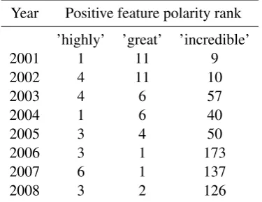
for negative values. We use such scaling later in the paper; however, for robustly detecting polarity shifts, we instead propose using feature polarity rankings. Such ranking is done by ordering fea-tures by their respective coefficients and assign-ing a rank to each feature. The highest coeffi-cient is rank 1, the second highest rank 2, and so on. This allows us to make direct comparisons be-tween several models trained on different subsets of data.

Year Positive feature polarity rank

’highly’ ’great’ ’incredible’

2001 1 11 9

2002 4 11 10

2003 4 6 57

2004 1 6 40

2005 3 4 50

2006 3 1 173

2007 6 1 137

2008 3 2 126

Table 2: Example feature ranks obtained by train-ing a logistic regression classifier on 32,000 re-views from each year.

Due to the exponential distribution of coeffi-cient values, as seen in Figure3, a cap on maxi-mal rank is placed such thatmax{rank} ≤3∗f, where f is the number of positive (or negative) features. If ranks would be uncapped, even the slightest decrease in coefficient value would dis-proportionately increase feature ranks. As a re-sult, rank and rank averages (used in predictive feature selection) would be much more influenced

by randomness of logistic regression, and hence, less interpretable. We argue that shifts in polarity are more precisely measured this way.

Figure 3: Distribution of coefficient values of 100 most positive and negative features obtained from models trained on data subsets from years 2001 to 2014. Coefficient values were scaled using Min-Max.

Using the feature polarity ranking described above, we analyze what shifts occur in individ-ual unigrams and bigrams. To do so, we again use random data subsets of 40,000 reviews and 80/20 splits. For each year spanning 2001 to 2014, we again generate three independent subsets to al-low for more robust results and less randomness caused by logistic regression. Each subset is used to train a classifier, and we compute the polarity ranks of all lexical features.

Once we have established the ranks of lexical features, we use linear regression to estimate the degree to which polarity has changed. Using the

p value of such a linear fit, we filter out non-significant changes wherep > 0.05. See Figure

4for examples of significant polarity shifts.

4 Models that are robust over time

Figure 4: Figure shows a sample of 3 bigrams and 2 unigrams, where significant degradation in pos-itivity was observed. Each color represents an in-dependently selected collection of random yearly subsets of reviews.

rank predictions to select features based on their expected polarity.

We use two methods for predictive feature se-lection, both relying on the predicted rate (or slope) of change in polarity and a metric of signif-icance that serves as a filtering mechanism. The methods used are:

• Difference of means:This method uses two mean polarity ranks - initial and final, to de-termine rate of change in feature polarity, and

whether the change is significant. Initial and final mean ranks are calculated using polarity ranks from individual years (i.e. how feature ranked in polarity as determined by model trained on data from that year). In our case, the training data spans 2001-2008 and differ-ence of means uses years 2001-2003 for the initial mean rank and 2006-2008 for the fi-nal mean rank. Furthermore, each feature to be included has to pass the following signifi-cance test:

|mean(06_mean(01−08)−mean(01₋₀₃₎ −03)|>0.05

The exact value can optionally be determined by experimentation, however in this experi-ment the significance threshold was set to 5% of the initial rank.

• Linear regression: We use linear regression to find the trend line of the feature polarity rank and use that in the decision process. As in previous method, yearly polarity ranks are used, however, instead of using only initial or final years we use the whole span of training data to obtain a linear fit. Thep-value calcu-lated during the fit is used as the significance threshold, where p < 0.05, for the feature polarity shift to be considered significant.

Using the methods described above, if signifi-cant temporal shift in polarity occurs, we obtain an expected rank for each such feature. This infor-mation is then used in predictive feature selection that is identical with both methods. First, a feature set of fixed sizeK(e.g.Kpositive andKnegative features) is created by looking at features that have the best average rank. Additionally, an extended supplement feature set is made of features that are in the next best category (i.e. mean rank K + 1

This new smaller set of features is then read from least polar expected rank, and while there is a fea-ture in thenext bestset we make a switch. Simply put, this procedure eliminates features predicted to lose polarity and features predicted to gain most polarity are included instead. Experiments show that number of features switched changes based on parameters (i.e. p-values, size ofK, etc.) from around 10% of the feature set forK = 100to 30% forK = 300.

4.1 Experiments

In the first experiment with temporally robust models, we used the difference of means to imple-ment predictive feature selection. The data used to create baseline accuracy was a random subset ofR

reviews, where, again,R = 40,000reviews were selected uniformly at random from years 2001 to 2008. After using 80/20 splits, a subset of 32,000 reviews was used to train a logistic regression clas-sifier, and following the training,Kmost negative and K most positive features were selected. In contrast to the baseline model, the temporally ro-bust model used the difference of means method to selectKnegative andKpositive features using predictive feature selection described in the sec-tion above. This setup was run 3 times with dif-ferent random subsets of data for both the baseline and the temporally robust model. The result ob-tained from the runs can be seen below in Figure

5and Table3.

Average model accuracies using 200 features

Test years Baseline Temp. robust

2010 0.828 0.834

2011 0.821 0.825

2012 0.834 0.839

2013 0.845 0.847

2014 0.845 0.85

Table 3: Each value in the table represents an av-erage accuracy of either a baseline or a temporally robust model tested on a data set of 8,000 reviews from the designated year. Each average is made over 3 experimental runs using different random subsets as training and test data (with no overlap between training and test). Every model used 100 positive and 100 negative features (i.e.K = 100). The predictive feature selection was implemented using the difference of means method.

Figure 5: The figure contains results from both the baseline and the temporally robust models trained with 200 features on 32,000 reviews. Upper part of the figure depicts model accuracies for all tested years and all 3 experimental runs; the lower part shows the average accuracy for each tested year. The difference of means method was used for pre-dictive feature selection.

Figure 6: The figure contains results from both the baseline and the temporally robust models trained with 800 features on 32,000 reviews. Upper part of the figure depicts model accuracies for all tested years and all 3 experimental runs; the lower part shows the average accuracy for each tested year. The difference of means method was used for the predictive feature selection.

As can be seen above in Figure6, significantly increased performance is present even in models that use increased number of features, i.e. from

K = 100toK = 400. Such a result suggests that predictive feature selection increases performance even when more features are used, and not only in the extremely sparse model with 200 features.

Figure 7: The figure contains results from both the baseline and the temporally robust models trained with 800 features on 32,000 reviews. Upper part of the figure depicts model accuracies for all tested years and all 3 experimental runs; the lower part shows the average accuracy for each tested year. The linear regression method withp-value filtering was used for the predictive feature selection.

features based on training data. In general, both methods -difference of meansandlinear regres-sion withp-value filter- achieve a similar perfor-mance, which is consistently better than our base-line model for all tested years and all tested num-bers of features, i.e.K ∈[100,200,400].

5 Conclusion

Large data sets for sentiment analysis are costly to create and are quite commonly a few years old. The performance of classifiers trained on such data sets decreases over time, as the interval between creations of test and training sets expands. This is, in part, due to a cumulative effect of individual lexical features going through amelioration, or pe-joration, which significantly changes their polarity over time. We call this effect fortemporal polarity shift.

To counter effects of these shifts, and improve the overall performance of a classifier, we devised two methods that allow us to predict the expected feature polarity. Using these methods, we imple-mented predictive feature selection, an approach, especially beneficial for sparse models, that se-lects a better feature set for the classifier using the expected polarity, rather than using the current most polar features in the training data. Tempo-rally robust models, i.e., the models using predic-tive feature selection, consistently achieve better accuracy than the baseline models, which suggest that negative effects of temporal polarity shifts can be countered to some degree.

References

John Blitzer, Mark Dredze, and Fernando Pereira. 2007. Biographies, Bollywood, Boom-boxes and Blenders: Domain Adaptation for Sentiment Clas-sification. InProceedings of ACL.

Paul Cook and Suzanne Stevenson. 2010. Automati-cally identifying changes in the semantic orientation of words. InLREC.

Ruining He and Julian McAuley. 2016. Ups and downs: Modeling the visual evolution of fashion trends with one-class collaborative filtering. In proceedings of the 25th international conference on world wide web, pages 507–517. International World Wide Web Conferences Steering Committee.

Julian McAuley, Christopher Targett, Qinfeng Shi, and Anton Van Den Hengel. 2015. Image-based recom-mendations on styles and substitutes. In Proceed-ings of the 38th International ACM SIGIR