Figure 1: On-off control system model Abstract—In order to implement a wireless sensor network in
process automation system it is needed to specify the sample number for the sensors. Because of the hardware and power supply limitations, wireless sensors are applied to discrete event control system. In wireless sensor network the highest sample number is restricted in comparison to the wired one. Moreover, the lowest sample number is also constrained by the limitations imposed by the control limits values. In this paper, relations between sample number and actuator’s frequency drift in discrete domain is formulated and presented. The central and autonomous sensor network structures are introduced. In addition, ways to compromise the sample number with the actuator’s frequency and control limits value are acknowledged. An approach to find the optimal sample number is proposed. It is shown when the sensor network becomes larger, autonomous network can partly compensate energy consumption increase by adding the sample number whereas central network does not support this feature.
Index Terms—Autonomous Network, Central Network, Sample Number, Wireless Sensor Network (WSN).
I. INTRODUCTION
Implementation of wireless sensor network (WSN) in automation process applications is one of the steps for establishing autonomous logistic systems [2]. WSN implementation in industrial automation systems such as Heating, Ventilation and Air Conditioning system (HVAC) is a research subject [1][3]. In order to implement WSN in an automation process application, two structures can be used: Autonomous structure and Central structure. In an autonomous network, wireless sensor nodes measure the environmental parameters. They are responsible for performing control tasks. If wireless sensor nodes require data from other sensors or actuators to perform these tasks, they ask for them. Sensors make decisions and send instructions to the actuators directly. In central network, sensors send their data to the center where the control tasks are performed. Afterward, the center sends the instructions to the actuators.
In this paper, WSN consists of nodes equipped with a wireless transceiver (CC2420), a tiny event driven
M.Sc Amir M Jafari is with the Institute for Microsensors, -actuators and -systems (IMSAS) at the university of Bremen, Bibliothekstrasse, 1 - D-28359 Bremen – Germany, (phone: +49 (0)421 218-4594; fax: +49 (0)421 218 - 4774; e-mail: [email protected]).
Prof. Dr. Ing Walter Lang is the professor and head of the Institute for Microsensors, -actuators and -systems (IMSAS) at the University of Bremen, Bibliothekstrasse, 1 - D-28359 Bremen – Germany (e-mail:[email protected]).
microcontroller from MSP 430 family and batteries for power supply. “Tmote sky” from “Moteiv” [4] is taken as sample of such nodes. The wireless transceiver is IEEE 815.15.4 standard compliant and its radio range is limited; therefore mesh topology is applied for establishing the network.
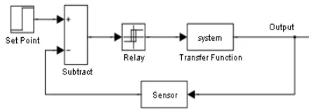
Because of the hardware and power supply limitations, wireless nodes are not suitable for continuous control systems. WSN is preferably used for On-off control system. In this application, two arbitrary limit values around the desired set-point are considered. When the system output is going to become greater than the upper limit value the actuator is turned off and when it is going to become less than the lower limit value, the actuator is turned on. Figure 1 shows a model for such system.
The question is what the sampling frequency should be for reading the output by the sensor. The sampling theorem [5] (Nyquist frequency criteria [6]) cannot be applied here because the relay is not a linear element and output is broken on the limits; therefore the output signal is not continuous while the sampling theorem works with continuous signal. On another hand sampling theorem does not offer any limitation from above for sample frequency while we will see that it is needed for WSN.
In a continuous control system the system output value is continuously compared with the limits and the instruction is sent to the actuator instantly. In a discrete domain, the sample is taken from output at each sample time. The decision for the actuator is made by comparing the sample values with the limits. In discrete domain there is a probability to go over the limit values. Suppose that a sample is taken just before the limits, the actuator status will not change until the next sample time. During this time the output goes beyond the limits, which causes inaccuracy and we call it error. In order to stay inside the continuous time limits interval and avoid such errors, the new limits are defined in a discrete domain. These limits in discrete domain are inside the continuous time limits interval. Since the actuator’s frequency is a function of the limits band width, it changes with the new limits value. This way the
Optimum Sample Number for Central and
Autonomous Wireless Sensor Network in
Process Automation Applications
Figure 4: Digitized system output Figure 2: Sample system step response
Figure 3: Control system with relay
sampling number is related to the actuator’s frequency in discrete domain. In section II, computation shows how the discrete limits value caused the actuator’s frequency drift.
In the next section the mathematical relation of actuator’s frequency drift in discrete domain, sample number and limits values is formulated for a first order linear time invariant (LTI) system. The behavior of the actuator frequencies for various sample numbers and limits interval is depicted.
In order to reduce the actuator frequency drift, sample numbers can be increased. On the other hand higher sample numbers in central and autonomous network causes more computation for node’s microcontroller and particularly in central network higher message transmission number which consequently results in more computation and transmission energy consumption. These considerations imply upper limit for the sample number whereas in wired network, the sample number can be increased high enough. Now the question is what is the optimum sampling frequency? An approach to a tradeoff between the sample number and energy consumption or message transmission number is offered in the third section.
II. SAMPLEFREQUENCYCALCULATION It is assumed that the transfer function of the system in figure (1) is H(s) expressed in(1). The step response of this system with Tn =3600 s is depicted in Figure (2). The set point value is assumed to be Y0 and the limit values are Yhc
and Ylc with equal distances from Y0. The On-off relay is implemented in the control loop (Figure (1)). Figure 3 shows the system step response for Yhc=0.7 and Ylc=0.5 for ten hours. The actuator On-off frequency in a continuous domain is calculated by (2).
)
1
(
1
)
(
s
=
T
×
s
+
H
n (1)c
f
Y
Y
Y
Y
T
t
t
f
nhc lc
lc hc
n
c
=
−
×
−
×
×
=
−
=
)
)
1
(
)
1
(
ln(
1
1
1 3
(2)
Equation (3) shows the recursive equation in a discrete domain when H(s) is mapped to the z-plane with sample time Ts and a normalized output. In this equation N is the sample number during Tc which is equal to inverse of fc computed in (2). Ts is the sampling period (fs sampling frequency) and c is defined in (2).
)
1
(
)
exp(
))
exp(
1
(
)
(
)
(
)
1
(
)
exp(
))
exp(
1
(
)
(
−
×
−
+
−
−
=
×
=
×
=
×
=
−
×
−
+
−
−
=
n
y
N
c
N
c
n
y
c
f
N
f
N
f
T
N
T
n
y
T
T
T
T
n
y
n c
s
s c
n s n
s
(3)
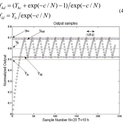
Assuming that the last sampling occurs just before the limit values; then the system output goes beyond the limit values up to the next sample time. This incident is counted as an error. In order to avoid such errors the new limit values are defined for discrete time system. These new values are equal to the samples of the output value on one sample period time before the limits Yhc and Ylc. These limits are called Yhd and Yld in (4). Considering this definition by lower sample number (Yhc - Yhd) becomes greater; consequently the limits interval (Yhd - Yld) becomes smaller. Smaller limit intervals lead to a greater actuator’s frequency fd. In other words, by moving to discrete domain with a low sample rate, actuator’s frequency increases and we have to deal with the actuator’s frequency drift.
)
/
exp(
)
/
exp(
)
1
)
/
exp(
(
N
c
Y
Y
N
c
N
c
Y
Y
lc ld
hc hd
−
=
−
−
−
+
=
[image:2.612.317.531.518.731.2] [image:2.612.77.289.552.725.2]Figure 5: A sample of actuator frequency ratio Figure 6: A sample of actuator frequency ratio Since Yhd should always be greater than Yld, a boundary
limit exists for sampling number N which is defined in (5). This is our first criteria for choosing sampling number. As an example for Yhc=0.7 and Ylc=0.5, N should be strictly greater than 3 (fs ≥ 4*fc). In figure 4 the digitized output for the above system with N=20 is depicted. The time axis is for ten hours. In comparison with figure 3 it can be seen that the actuator’s state changes 20 percent more than its value in a continuous domain of the control system.
))
1
ln(
(
Y
lcY
hcc
N
>
−
+
−
(5)In autonomous WSN when the system output reaches its limits, sensor sends an instruction message to the actuators. In figure 4 it can be seen that the number of message transmissions is double the number of the actuator’s status changes (i.e. one message for on-off and one message for off-on transient states). It denotes that the message transmission number is proportional to the actuator’s frequency. Since reduction of the sample number decreases the discrete limit intervals and it leads to amplifying the actuator frequency, consequently the number of message transmissions increases. By raising the sample number, the microcontroller occupancy and energy consumption increases too. This phenomenon causes losing more messages during the routing of other sensor’s messages in addition to increasing the process energy consumption. Therefore the sample number should be compromised in a way that it is neither very small that causes the increase in the actuator’s frequency and message transmission nor so large that the microcontroller becomes too occupied and the process energy consumption increases highly. This process is discusses in the next section.
In a central WSN, sensor sends message to the center at each sample time (Figure4). Increasing the sample number, raises the message transmissions number directly which causes more transmission energy consumption and high network traffic. Moreover high frequency is not beneficial for actuator’s life time as well. Reduction of the sample number leads to the rising of actuator’s frequency which means the center should send more messages to the actuator. Increasing the sample number in central network causes more transmission energy while in autonomous network it leads to more process energy consumption. In addition
process energy consumption is much smaller than transmission energy consumption. Therefore sample number in an autonomous network can be greater than its value in a central network which implies that with the same energy consumption, lower actuator frequency and better control quality can be achieved with autonomous configuration.
1 ) )
1 (
) ) / )(exp( 1 ) / exp( (
ln(
) (
−
− ×
− − −
− +
= −
= Δ
hc lc
lc hc
c c d c
Y Y
Y N c N
c Y
c f f f f f
(6)
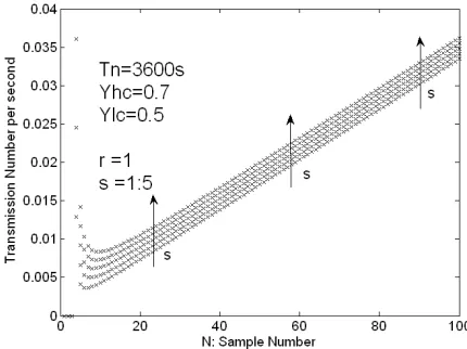
The normalized difference between actuator’s frequencies in continuous and discrete domain is shown in (6). By this equation the sample number and actuator’s frequency can be optimized. The graph of (6) is depicted for Yhc=0.7, Ylc=0.5 and Tn =3600 s in figure 5. It is computed by (5) that for these values, N must be greater than 3. For N=4 the actuator’s frequency increases to 16.67 times (1667 percent) of its frequency in continuous domain (figure 5). As it is mentioned in the previous section it indicates that 16 times more instruction messages should be sent to the actuator to turn on or off. This oscillation is not reasonable for actuator either. Therefore by increasing the sample number to 20, the actuator’s frequency drift is about 20 percent which could be more acceptable considering the process and 1667 percent with pervious sample number. By increasing sample number from N=30 to N=50, the actuator’s frequency decreases just about 6.5% implying 66.66% increase of process energy consumption, 66.66% increase of the node’s microcontroller occupancy in autonomous network and the same percent increase of message transmission in central network. This increase (from N=30 to N=50) sounds not very helpful. In the next section, Equation 6 shows that the sample number is compromised with actuator oscillation which is proportional to message transmission number.
[image:3.612.77.291.559.720.2]Figure 8: Number of message transmission corresponding to each sample number in central structure of figure7.
Sensor Center
Actuator r hops
s hops
[image:4.612.318.532.54.199.2]Figure 7: Central network structure
Figure 9: Number of message transmissions corresponding to each sample number with different hops number from center to actuator in central structure of figure 7.
[image:4.612.315.530.540.701.2]Table 1: Sample number corresponding to hops number from center to actuator
Table 2: Sample number corresponding to hops number from sensor to center
s Minimum g N r Minimum g N
1 0.0036 6 1 0.0036 6
2 0.005 8 2 0.0056 6
3 0.0062 8 3 0.0074 5
4 0.0073 9 4 0.0091 5
5 0.0084 10 5 0.0107 5
6 0.0094 10 6 0.0123 5
7 0.0104 11 7 0.014 5
8 0.0113 11 8 0.0156 5
9 0.0123 12 9 0.0173 5
1
0 0.0132 12
1
0 0.0189 5
20
percent actuator’s frequency drift ((∆f / fc) ≤ 0.2) is acceptable for the sensor and actuator, ∆Y would be 0.18.
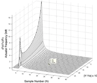
Figure 6 is derived from (7) with Y0=0.7. This figure shows that by changing the limit values to maximum possible numbers, the actuator’s frequency differs about 50 percent. On the other hand, for small N, increasing the interval does not necessarily lead to a lower frequency difference. Utilizing (7) offers the trade off option between three parameters: control limits, actuator’s frequency and sampling number.
) )) 1
( ) (( )) 1
( ) (( ln(
1 ) )
1 ( ) (
) )
/ )(exp( 1 ) / exp( (
ln(
) (
0 0
0 0
0 0
0 0
y Y y Y y Y y Y c
y Y y Y
y Y N c N
c y
Y
c f f f f
f c d c c
Δ − − × Δ + Δ
+ − × Δ + =
−
Δ − − × Δ −
Δ + − − − − + Δ +
= −
= Δ
(7)
III. SAMPLENUMBERSELECTION
In central and autonomous networks, message transmission number is related to the sample number and actuator frequency. The sample number can be selected in compromise with the transmission number in central network and energy consumption in autonomous network.
A. Central Network
For central network, the structure in figure 7 is considered. In the network shown in figure 7 the sensor measures the environment parameter in each sample time and sends it to the center through r hops. The center checks the sensor value; if it is greater than the upper limit value it sends a message to the actuator to turn it “on”. When the received sensor value is less than the lower limit, it sends a message to turn the actuator “off”.
In figure 7 with the sample number of N, the number of
message transmissions from the sensor to the center during time T is equal to T/Ts×r = ((T×N)/Tc)×r. At the same time interval T, the number of instruction message transmissions from the center to the actuator is equal to (T/Td) ×2×s = (T×(p(N)+1)/Tc)×2×s. By adding these two values the total number of transmissions in unit time is equal to (8).
c
f
s
N
p
r
N
s
r
N
g
(
,
,
)
=
(
×
+
(
(
)
+
1
)
×
2
×
)
×
(8)The graph of (8) with r=s=1 is given in figure 8 with the system parameters of the pervious section. The function is minimum at N=6. Considering the minimum of the transmission numbers, the best sample number is equal to 6 concerning to Tn & Yhc & Ylc. It indicates that the sample should be taken at every Ts=Tc / N ≈ 508 s.
[image:4.612.77.296.658.727.2]Figure10: Number of message transmissions corresponding to each sample number with different number of hops from the sensor to the center in central structure.
Sensor
Actuator
r hops
[image:5.612.76.270.553.698.2]Figure 11: Autonomous network structure
Table 3: Maximum N values for which inequality of 12 is valid for different r.
r 1 2 3 4 5 6 7 8 9 10
N 12 16 19 21 23 25 27 28 30 31
ratio changes to g(12,1,10) / g(6,1,1) ≈ 3.55. These two ratios comparison shows that by changing the sample number to 12, the message transmission number is reduced about 27 percent. It means adding intermediate nodes between the center and actuator leads to the energy consumption increase which is partly compensated by increasing the sample number. This is an advantage of finding the sample number corresponding to the minimum of equation g(N,r,1s).
From another angle we hold the s=1 and start to increase r one unit at a time. Table 2 shows that when the number of hops increases, N does not change significantly in order to compensate the increase in the number of hops. N should be reduced but its value is limited by (5). This claim can be verified by inequality 9. In this inequality the right side shows the ratio of message transmission increase when the number of hops between the sensor and the center increases. The left side represents the message transmission increase when the number of hops between the actuator and the center increases. From this observation and comparison of figure 9 & 10, it is concluded that in central network it is more efficient to choose the center closer to the sensor than the actuator. Practically it is more effective to consider that the center should be closer to the node with higher loads to deliver. In continuance, if we take r=0 (sensor instead of center), the result is still valid. This network with r=0 is the same as an autonomous network. It implies that when the number of hops increases, the autonomous network has less transmission number and consequently works better.
[
g(5,10,1) g(6,1,1)] [
> g(12,1,10) g(6,1,1)]
≅5.25>3.66 (9)Finally, if there are r hops from the sensor to the center and s hops from the center to the actuator, the proper sample number is where g is minimal. As an example for r=3 and s=7, N corresponding to the minimum g is equal to 8.
B. Autonomous network
For autonomous structure we consider the structure shown in figure 11. The sensor in this figure measures the environment parameter at each sample time. Then the sensor compares it with the limit values; if it is greater than the upper limit, the sensor sends a message to the actuator to turn it “off” and when it is less than the lower limit, the sensor sends a message to turn it “on”. In this paper it is
assumed that the average of the process energy for taking a sample or finding the next node by routing algorithm is fixed and it is considered as the unit for energy consumption measurement. Another assumption is that the transmission energy from one node to another is equal to e=10 times of process energy (energy consumption unit).
c
f
r
N
p
r
N
h
(
,
)
=
(
(
)
+
1
)
×
2
×
×
(10)In figure 11 the number of transmissions for N in time T is equal to (T/Td)×2×r= (T×(p(N)+1)/Tc) ×2×r and in unit time it is equal to the function h in (10) (h(N,r)=g(N,0,r)).
As N increases from N=i to N=i+1, p(N) or the actuator frequency drift with respect to figure 5 decreases. This reduction causes the reduction of h or the message transmission number. Equation 11 formulates the reduction of the transmission numbers which is equivalent to ∆h*e of the process energy consumption reduction. Reduction of transmission numbers also causes reduction of the process energy for forwarding messages in intermediate nodes. We call the summation of these two energy consumption reductions as saved energy. From another side by increasing the N, the process energy consumption increases in order to take more samples. We look at this energy consumption increase as cost energy. These concepts entail that by increasing N, the transmission number decreases but N’s higher limit value is also restricted. Therefore optimal N is where the saved energy is still greater than the cost energy, which is formulated in (12). Optimal sample number is maximum N so that the inequality 12 becomes valid.
c i
i c i
i
f
r
p
f
r
i
p
i
p
r
i
h
r
i
h
h
×
×
×
Δ
=
×
×
×
+
−
=
+
−
=
Δ
+ +
2
2
))
1
(
)
(
(
)
,
1
(
)
,
(
1 1
(11)
0
2
)
1
)
1
((
))
(
1
(
)
1
(
1
×
+
×
−
×
×
−
>
Δ
=
×
−
+
−
−
×
Δ
+
×
Δ
+
c c
i i
c
f
f
r
e
p
f
i
i
r
r
h
e
h
(12)
For Yhc=0.7, Ylc=0.5 and Tn =3600 s table 3 shows N as in previous section corresponding to each r. For example when r=2 then N=15 and Ts=Tc/N ≈ 190 s is the optimum sample number.
about 150% in comparison to the continuous time. If this oscillation is not acceptable, as an criteria, N can be increased to 8 and actuator’s frequency drift reduces to about 80%.
IV. CONCLUSIONS
In this paper it is presented that the sensor’s sample number selection in WSN for process automation application is not as straightforward as common methods used in wired network. Sample number has impacts on the actuator’s frequency, number of message transmissions and sensor node’s microcontroller occupancy. It has been shown that actuator’s frequency gets closer to its value in continuous domain by a higher sample number. Small sample number causes the actuator’s frequency increase and consequently reduction of actuator’s life time.
Moreover, this phenomenon increases the requirement for sending instructions to the actuator. In a wired control systems this problem can be solved by increasing the sample number to a high enough value. But in WSN increasing sample number causes side problems. In autonomous WSN, higher sample number increases microcontroller occupancy and process energy consumption. In central WSN, higher sample number leads to more message transmission energy consumption in the nodes which are supplied by batteries.
In this paper the above constrains are taken into account and an approach for finding the sample number corresponding to the actuator’s frequency drift is offered. In addition a tradeoff technique between the actuator’s frequency, sample number and limits value interval is introduced. For finding the optimum sample number in central WSN a function is given and the optimum N is the corresponding variable to the minimum value of this function. With the same function it is shown that when the number of hops between nodes increases, the autonomous network can offer less message transmission number by higher sample number and consequently better functionality. This property of autonomous network is known as an advantage of autonomous configuration. An inequality is given for autonomous network which states difference between the saved and cost energy. The optimal sample number is where this difference becomes minimal.
ACKNOWLEDGMENT
Amir Jafari thanks Mahvash Nejad from San Jose state university for proof reading of this paper.
REFERENCES
[1] Masato Yamaji, Yosuke Ishii, Tomomi Shimamura, and Shuji Yamamoto, Wireless Sensor Network for Industrial Automation, 5th International Conference on Networked Sensing Systems, 2008. Date: 17-19 June 2008, pp: 253 – 253.
[2] R. Jedermann, C.Behrens, R.Laur,W. Lang, Intelligent containers and
sensor networks, Approaches to apply autonomous cooperation on
systems with limited resources. In: Hülsmann, M.; Windt, K. (eds.):
Understanding Autonomous Cooperation & Control in Logistics – The Impact on Management, Information and Communication and Material Flow. Springer, Berlin, 2007, pp. 365-392.
[3] Fredrik O¨, Erik Pramsten, Daniel Roberthson, Joakim Eriksson, Niclas Finne, Thiemo Voigt, Integrating Building Automation Systems and
Wireless Sensor Networks. SICS Technical Report T2007:04 May
2007.
[4] MoteivCorporation.tmote-sky-datasheet-02.www.moteiv.com, 2006. [5] Katsuhiko Ogata, Discrete-Time Control Systems, Second edition,
Prentice-Hall Inc, 1995.pp 90-98.
[6] Alan V.Oppenheim, Ronald W.Schaffer, John R.Buck, Discrete-Time
Signal Processing, Second edition, Prentice-Hall Inc, 1999. pp