Average case analysis of algorithms for the maximum subarray problem

(1)

AVERAGE CASE ANALYSIS OF ALGORITHMS FOR THE MAXIMUM

SUBARRAY PROBLEM

A thesis submitted in partial fulfilment of the requirements for the Degree

of Master of Science in Computer Science

in the University of Canterbury

by Mohammad Bashar

University of Canterbury

(2)

(3)

Examining Committee:

• Prof. Dr Tadao Takaoka, University of Canterbury (Supervisor) • Associate Prof. Dr Alan Sprague, University of Alabama

(4)

(5)

(6)

(7)

Abstract

Maximum Subarray Problem (MSP) is to find the consecutive array portion that maximizes the sum of array elements in it. The goal is to locate the most useful and informative array segment that associates two parameters involved in data in a 2D array. It’s an efficient data mining method which gives us an accurate pattern or trend of data with respect to some associated parameters. Distance Matrix Multiplication (DMM) is at the core of MSP. Also DMM and MSP have the worst-case complexity of the same order. So if we improve the algorithm for DMM that would also trigger the improvement of MSP. The complexity of Conventional DMM is O(n3). In the average case, All Pairs Shortest Path (APSP) Problem can be modified as a fast engine for DMM and can be solved in O(n2 log n) expected time. Using this result, MSP can be solved in O(n2 log2 n) expected time. MSP can be extended to K-MSP. To incorporate DMM into K-MSP, DMM needs to be extended to K-DMM as well. In this research we show how DMM can be extended to K-DMM using K-Tuple Approach to solve K-MSP in O(Kn2

(8)

(9)

Acknowledgments

The last one and half year of my academic life has been a true learning period. This one page is not adequate to thank all those people who have been supporting me during this time.

Firstly, I would like to thank my supervisor Professor Tadao Takaoka, who gave me the opportunity to do this research and his continuous assistance, guidance, support, suggestions and encouragement have been invaluable to me. I honestly appreciate the time and effort he has given me to conduct my research.

Secondly, I would like to express my gratitude to my lab mates and friends who had made my university life more enjoyable and pleasant by sharing their invaluable time. I specially thank Sung Bae, Lin Tian, Ray Hidayat, Oliver Batchelor, Taher Amer and Tobias Bethlehem for their priceless help and encouragement.

(10)

(11)

List of Figures

Figure 1: Given input array...2

Figure 2: Converted input array...3

Figure 3: Prefix sum...9

Figure 4: K-MSP example ...12

Figure 5: Two (3, 3) matrices ...15

Figure 6: 3-layered DAG of two (3, 3) matrices ...16

Figure 7: Resulting matrix C...16

Figure 8: Resulting matrix containing the first shortest distances...18

Figure 9: Resulting matrix containing the second shortest distances ...19

Figure 10: Resulting matrix containing the third shortest distances...19

Figure 11: (m, n) array ...23

Figure 12: Solution set expansion process ...34

Figure 13: Two vertices pointing to same candidate...35

Figure 14: Intermediate stage of solution set expansion process...36

Figure 15: Visualizing set S, U and U-edge ...41

Figure 16: 3-layered DAG of two (n, n) matrices ...45

Figure 17: Intermediate stage of set W...47

Figure 18: Visualization of array T...59

Figure 19: (a, a) array at the bottom of the recursion ...80

Figure 20: Four-way recursion and 6 solutions...81

Figure 21: X + Y problem solving in O(K log K) time ...83

Figure 22: Binary tournament tree...91

Figure 23: Visualization of the intermediate recursion process...95

Figure 24: Strip Visualization...96

Figure 25: Scope and position of a maximum subarray solution ...97

Figure 26: (n,n) array yielding O(n2) strips and O(n2) subarrays per strip ...98

Figure 27: APSP Problem time measurement...103

Figure 28: DMM time measurement ...105

Figure 29: MSP time measurement ...106

Figure 30: K-DMM time measurement ...108

Figure 31: K-MSP time measurement (comparison between Conventional and K-Tuple Approach) ...110

(16)

(17)

List of Tables

Table 1: APSP Problem time measurement ...103

Table 2: DMM time measurement...104

Table 3: MSP time measurement...105

Table 4: K-DMM time measurement ...107

(18)

(19)

Chapter 1 Introduction

(20)

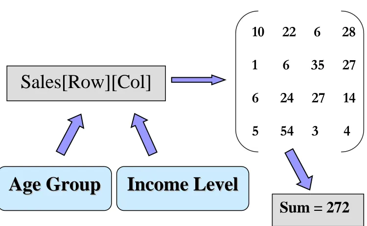
input array would yield more precise evaluation of the sales trends with respect to age groups and income levels of purchasers.

The formulation of the problem in terms of the example matrix below is as follows:

Suppose the sales record of an arbitrary product is given in the following 2-dimensional input array.

10 22 6 28

1 6 35 27

6 24 27 14

[image:20.612.134.509.312.543.2]

5 54 3 4

Sales[Row][Col]

Figure 1: Given input array

If we consider the given input array with all positive numbers the trivial solution for the MSP is sum of the whole array which is 272 in this example.

A

Ag

ge

e

G

r

o

up

u

p

In

I

nc

co

om

me

e

L

Le

ev

ve

el

l

(21)

[image:21.612.159.518.264.484.2]

As we explained earlier, to avoid this trivial solution we subtract the mean value of the array elements from each individual element of the same array. In the preceding example, the mean value of the array elements is 17 (as 272/16 = 17). In the following array we represent the modified input array after subtracting the mean value from each individual values and we find the maximum subarray on this modified input array.

Figure 2: Converted input array

In Figure 2, we can observe the maximum subarray is defined by the rectangular array portion. The position of this subarray in the main array can be tracked as (2, 2) which corresponds to the upper left corner and (4, 3) which corresponds to the lower right corner. By tracking the maximum subarray in

Sales[Row][Col]

A

g

e

G

r

o

u

p

I

n

c

o

m

e

L

e

v

e

l

-7 5 -11 11

-16 -11 18 10

-11 7 10 -3

-12 37 -14 -13

(22)

this way, we can find the range of age groups and income levels that contribute to the maximum sales.

The other possible application for MSP is Graphics. The brightest portion of an image can be tracked by identifying the maximum subarray. For example, a bitmap image consists of non-negative pixel values. So we need to convert these non-negative pixel values into an accumulation of positive and negative values by subtracting the mean or average from each pixel value. By applying MSP into these modified pixel values the brightest portion in the image can be easily traced.

1.1Maximum Subarray Problem Extension

MSP can be extended to K-MSP where the goal is to find K maximum

subarrays. K is a positive number which is between 1 and 4

mn

(m+1)(n+1)

where m and n refer to the size of the given array. We explain in details in Chapter 2 with example how K is bounded by this number for a given array of size (m,n).

(23)

All maximum subarrays that have been detected in a given array can be overlapped with each other.

1.2 A Real-life Significance of K- Maximum Subarray Problem

A real-life example of K-MSP could be a product leaflet delivery example. Let’s assume we own a company and we would like to deliver information of the new products of our company on a leaflet to our potential consumers. We also would like to target our potential customers from the area of the city which is densely populated. After detecting the densely populated area of the city with the help of MSP we realized that this area is not physically accessible due to road construction work. Thus we need to identify the second most densely populated area of the city for our new products leaflet delivery. If this is also not accessible due to some reason we need to identify the third most densely populated area of the city and so on. The interesting observation here is that the first maximum subarray is available to us but practically it may not be feasible to use all the time. And thus, K-MSP plays its role to overcome this limitation.

1.3 Research Scope

(24)

power of 2. The array size is represented by m and n. If m and n are not powers of 2 we can extend our framework to the case where m and/or n are not power of 2. Also all unspecified logarithms should be considered as binary.

1.4 Research Objectives

The objectives of this research are:

1. To develop efficient algorithms for K-MSP.

2. To do the average case analysis of algorithms for MSP and K-MSP.

3. To compare and evaluate existing algorithms with new algorithms for K -MSP.

1.5 Research Structure

(25)

(26)

(27)

Chapter 2 Theoretical Foundation

In this chapter we present a number of core concepts that are related with MSP. As we further discuss the related work of MSP in the next chapter it will become transparent how these concepts are related with MSP.

2.1 Research Assumptions

All numbers that appear in the given (m, n) array are random and independent of each other.

2.2 Prefix Sum

The prefix sum of an array is an array in which each element is obtained from the sum of those which precede it. For example, the prefix sum of:

(4, 3, 6, 7, 2) is (4, 4+3, 4+3+6, 4+3+6+7, 4+3+6+7+2) = (4, 7, 13, 20, 22)

For 2D cases, the prefix sum of

=

1 -5 9

8 -4 3

4 3 -2

1 -4 5

9 0 12

13 7 17

(28)

The prefix sums s[1..m][1..n] of a 2D array a[1..m][1..n] is computed by the following algorithm. Mathematically, s[i][j] is the sum of a[1..i][1..j].

______________________________ Algorithm 1: Prefix Sum Algorithm 1: for i := 0 to m

2: for j := 0 to n

3: s[i][j] = 0; 4: column[i][j] = 0; 5: end for;

6: end for; 7: for i := 1 to m

8: for j := 1 to n

9: column[i][j] = column[i –1][j] + a[i][j]; 10: s[i][j] = s[i][j –1] + column[i][j]; 11: end for;

12: end for;

_______________________________

The complexity of the above algorithm is straightforward. It takes O(n2) time to compute the 2D prefix sum where m = n.

2.3 Maximum Subarray Problem

(29)

2.3.1 Exhaustive Method

The brute force or exhaustive algorithm to calculate maximum subarray is as follows:

___________________________________ Algorithm 2: Exhaustive MSP Algorithm

1: max = – 999; 2: for i := 1 to m

3: for j := 1 to n

4: for k := 1 to i

5: for l := 1 to j

6: currentmax = s[i][j] – s[i][l] – s[k][j] + s[k][l]; 7: if currentmax > max)

8: max = currentmax; 9: end if;

10: end for; 11: end for; 12: end for; 13: end for;

___________________________________

(30)

2.3.2. Efficient Method

Takaoka [1] described an elegant method for solving MSP. In Chapter 3 we investigate this algorithm in details. This research is primarily based on Takaoka’s MSP algorithm which solves MSP by applying divide-and-conquer methodology.

2.4 K-Maximum Subarray Problem

MSP was extended to K-MSP by Bae and Takaoka [2]. This is an extension of the original problem. Instead of searching for only one maximum subarray we search for K maximum subarrays. For example, in Figure 4 we have identified 2 maximum subarrays, as K is 2.

1 5 6 -28

-1 -6 35 27

-54 -24 27 14

1 2 3 4

Sum = 110

K

= 1

K

= 2

Sum = 103

(31)

2.4.1 Exhaustive Method

The brute force or exhaustive algorithm to calculate K maximum subarrays is as follows:

_____________________________________ Algorithm 3: Exhaustive K-MSP Algorithm

1: for r := 1 to K

2: max[r] = – 999; 3: for i := 1 to m

4: for j := 1 to n

5: for k := 1 to i

6: for l := 1 to j

7: currentmax = s[i][j] – s[i][l] – s[k][j] + s[k][l];

8: if (currentmax > max[r] AND currentmax’s co-ordinates (i, j, k, l)

9: differ from all maximum subarrays co-ordinates (i, j, k, l) that 10: we have computed previously)

11: max[r] = currentmax; 12: end if;

13: end for; 14: end for; 15: end for; 16: end for; 17: end for;

_____________________________________

(32)

to K for K-MSP. Also max is a list to hold K-maximum sums. The complexity of the above algorithm is O(Kn4) where m = n.

2.4.2 Efficient Method

Takaoka and Bae [2] modified Takaoka’s [1] MSP algorithm to deal with K -MSP. We also modify Takaoka’s [1] MSP algorithm in Chapter 4 based on K -Tuple Approach. In Chapter 5, we modify Takaoka’s [1] MSP algorithm once again based on Tournament Approach.

2.5 Distance Matrix Multiplication

By translating prefix sums into distances, we can solve MSP by Distance Matrix Multiplication (DMM) and we will show this in the next chapter. Now we describe DMM.

The purpose of DMM is to compute the distance product C = AB for two n -dimensional matrices A = [ai, j] and B = [bi,j] whose elements are real numbers.

ci,j = minnk=1 { ai,k + bk,j }

The meaning of ci,j is the shortest distance from vertex i in the first layer to

(33)

the second layer to j in the third layer is bi,j. The above min operation can be

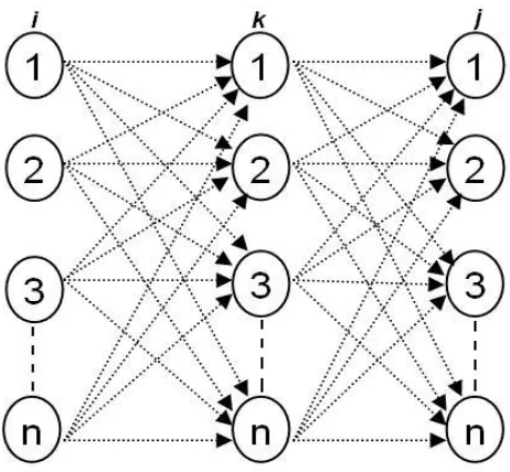
replaced by max operation and thus we can define a similar product, where we have longest distances in the 3-layered graph that we have described above. This graph is depicted in Figure 6.

Suppose we have the following two matrices A and B.

A

B

3 5 8

4 5 6

1 2 6

-2 0 8

4 7 2

2 9 -3

Figure 5: Two (3, 3) matrices

(34)

3

2

1

3

2

1

3

2

-3 9 7

4

8 -2

0

2

6 1

6 5

4 8

3

5

1

Figure 6: 3-layered DAG of two (3, 3) matrices

Then the resulting matrix C would look like as follows:

1 3 5

2 4 3

-1 1 3

[image:34.612.178.538.109.352.2]

C =

(35)

2.5.1 Conventional DMM

The algorithm for DMM which uses the exhaustive or brute-force method is termed as Conventional DMM in this research. In the following we give the

min version of DMM algorithm where m = n.

______________________________________ Algorithm 4: Conventional DMM Algorithm 1: for i := 1 to n

2: for j := 1 to n

3: C[i][j] = 999; //infinite value 4: for k :=1 to n

5: if(A[i][k] + B[k][j] < C[i][j] ) 6: C[i][j] = A[i][k] + B[k][j]; 7: end if;

8: end for; 9: end for; 10: end for;

______________________________________

The complexity of the above algorithm is O(n3) due to triple nested for loops. So this is obviously a naïve approach. For a big data set this approach would not be efficient.

2.5.2 Fast DMM

(36)

algorithm) and named this new algorithm as Fast DMM. This algorithm is scrutinized in Chapter 3 which takes O(n2 log n) time.

2.6 K-Distance Matrix Multiplication

DMM can be extended to K-DMM as follows:

ci,j = min [K] { ai,k + bk,j | k=1..n }

where min[K]S is the set of K minima of S ={ ai,k+ bk,j|k=1..n}. cijis now a set

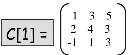
of K numbers. The intuitive meaning of K-DMM of MIN-version is that cij is the K-shortest path distances from i to j in the same graph as described before. Let cij[k] be the k-th of cijand C[k] = [cij[k]]. In the above example k runs from

1 to 3 (as n = 3). So we have 3 different output matrices for C and these are shown in Figure 8, 9 and 10.

1 3 5

2 4 3

-1 1 3

[image:36.612.232.454.467.562.2]

C[1] =

(37)

9 12 7

8 12 7

6 9 4

[image:37.612.224.443.103.213.2]

C[2] =

Figure 9: Resulting matrix containing the second shortest distances

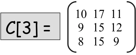
10 17 11

9 15 12

8 15 9

C[3] =

Figure 10: Resulting matrix containing the third shortest distances

2.6.1 Conventional K-DMM

The exhaustive or brute-force method to find the K-DMM is termed as Conventional K-DMM algorithm in this research. In the following we give this algorithm where m = n.

______________________________________ Algorithm 5: Exhaustive K-DMM Algorithm 1: for i:= 1 to n

2: for j := 1 to n

3: select K minima of {ai1 + b1j,……,ain + bnj} 4: end;

5: end;

[image:37.612.224.451.267.359.2]

(38)

We assume binary heap is used for the priority queue and insertions of new elements into the heap are done in bottom-up manner. Then line 1 and line 2 would contribute O(n2) complexity because of doubly nested for loops. On line 3, before we insert and select K items from the heap we must initialize the heap. This would cost us O(n) time for n items. Then selection of K items from

n items in the heap would cost us O(K log n) time. So the complexity of the above algorithm becomes O(n2 (n + K log n)) which is equivalent to O(n3 + n2 K log n).

2.6.2 Fast K-DMM

Takaoka’s Fast DMM can be extended to find K-DMM in an efficient manner. In Fast DMM, APSP Problem is used as a fast engine where we establish the shortest path from every source to every destination. When we extend this to

K-DMM, the idea is to establish K-shortest paths from every source to every destination. We modify Takaoka’s Fast DMM by extending it to Fast K-DMM and we present this new algorithm in Chapter 4.

2.7 Lemmas

(39)

2.7.1 Lemma 1

Suppose that in a sequence of independent trials the probability of success at each trial is p. Then the expected number of trials until the first success is 1/p.

Proof: From the properties of the geometric distribution in [4].

2.7.2 Lemma 2

Suppose that in a sequence of independent trials the probability of each of n

mutually exclusive events is 1/n. Then the expected number of trials until all n

events have occurred at least once is approximately n ln (n), where ln is natural logarithm.

Proof: From Lemma 1 and the results given in [5].

2.7.3 Lemma 3

x

− 1

1

≤ 1 + 2x for 0 ≤ x ≤ ½

Proof: The given condition is:

0 ≤ x ½ ≤

(40)

⇒1 – 2x 0 or ≥ x ≥ 0

⇒ x (1 – 2x) 0 ≥

⇒ x – 2x2 0 ≥

⇒1 + 2x – x – 2x2 –1 0 ≥

⇒ (1 + 2x)(1 – x) 1 ≥ (proved)

2.7.4 Lemma 4

0 + 1 + 2 +……. + K – 1 = 2

) 1 (K− K

2.7.5 Lemma 5

If an array size is (m, n) then the number of maximum subarrays is bounded by O(m2n2) or O(n4) where m = n.

Proof: For an arbitrary array of size (m, n) we can establish the following inequality.

K ≤

∑∑

= =

m

i n

j

ij

1 1

(41)

K ≤

∑∑

= =

m i

n j

ij

1 1

∑

=

∑

= n j m i

j i

1

1 2

m

(m+1) 2

n

(n+1) = 4

mn

(m+1) (n+1)≤ O(m2n2)

Now we consider the following example where m = n = 2.

Figure 11: (m,n) array

K = 4

mn

(m+1)(n+1)= 4

2 2x

(2 + 1)(2+1) = 9 ≤ O(m2n2 = 16)

Using the above formula we can find the possible number of K subarrays for a given array of size (m,n).

2.7.6 Lemma 6

Part A: Now we would like to establish a formula by which we can find the

required array size of (m,n) for a given K.

[image:41.612.256.386.218.325.2]

(42)

4

mn

(m+1)(n+1) ≥K

If we consider the case where m = n then the above inequality can be rewritten as follows:

⇒ 4

2

m

(m+1)2 ≥ K

⇒ m2 (m+1)2 ≥ 4K

⇒ m (m+1) ≥ 2 K

⇒ m2 + m – 2 K ≥ 0

⇒ m =

2 8 1

1± + K

−

For example, if K = 16 we would like to find the required array size of (m, n) so that we can return 16 subarrays. We plug in K = 16 into the above equation and round up to the nearest integer. Since m can’t be negative we only take the positive value and we get 2.37. Then we take the ceiling of this value and get

m = 3. That is we consider m =

⎥ ⎥ ⎥ ⎤ ⎢

⎢ ⎢

⎡₋ ₊ ₊

2 8 1

1 K

. To have K subarrays

(43)

3) there are in fact exactly 36 subarrays (using Lemma 5) available. But we only select 16 subarrays out of 36 subarrays when K = 16.

Part B: Let b is the exact solution for the quadratic equation. That is b =

2 8 1

1+ + K

−

. Let a = ceiling (b), which means a < b + 1. We can further

rewrite this as a – 1 < b. Now using Lemma 5, we can establish the following inequality by considering the case where m = n and setting m = a –1 and m =

b. 2 2 ) 1 1 ( 4 ) 1 ( − ₋ ₊ a a

< 2

2

) 1 ( 4 b+

b

< K

⇒ 2 2 ) 1 1 ( 4 ) 1 ( + − − a a

< K

⇒ 2

2

) 1 ( 4 a−

a

< K

⇒ ( 2 1)

4 2 2 + − a a a

< K

⇒

4

2 3 2

4

a a

a − +

(44)

⇒

4

2 3 2

4

a a

a − +

+ a3 < K + a3 (adding a3 on the both side)

⇒

4

2 3 2

4

a a

a + +

< K + a3

⇒ 4 ) 1 2 ( 2

2 + +

a a a

< K + a3

⇒ 4 ) 1 ( 2 2 ₊ a a

< K + a3

In the above we have established the fact that when we consider array size of (a, a) instead of exact size of (b, b) there are at most K + a3 subarrays available.

2.7.7 Lemma 7

Endpoint independence holds for the DMM with prefix sums for a wide variety of probability distribution on the original data array.

Proof: The basic randomness assumption in this thesis is the endpoint

(45)

Let us take a 2 dimensional array given by a[1][1],….,a[n][n]. Let us assume

a[i][j] are independent random variables with prob{a[i][j] > 0} = ½. Then we have

prob{a[1][j] +.…..+ a[i][j] > 0} = ½ ---(I)

Also let b[j] = a[1][j] +.…..+ a[i][j] ---(II)

Let prefix sum s[i][j] = s[i][j-1] + b[j]

Now we ignore i and thus we can write

s[j] = b[1] + b[2] +.…..+ b[j] ---(III)

Now from (I) & (II) we have

prob{b[j] > 0} = ½ ---(IV)

Now we consider another variable k and using (III) we can write

s[k] = b[1] + b[2] +.…..+ b[k] ---(V)

For k < j, from (III) & (V) we have

(46)

As in (IV) we have shown b[j] are independent random variables with

prob{b[j] > 0} = ½ then we can write

prob{b[k + 1] +.…..+ b[j] > 0} = ½ and thus

prob{s[k] < s[j]} = ½

Hence we have any permutation of s[1], .…..,s[n] with equal probability of ! 1

n ,

(47)

Chapter 3 Related Work

In this chapter we review and discuss previous works that were carried out by other researchers on MSP.

3.1 Main Algorithm of MSP based on DMM

MSP was first proposed by Bentley [6]. Then it was improved by Tamaki and Tokuyama [8]. Bentley achieved cubic time for this algorithm. Tamaki and Tokuyama further achieved sub-cubic time for a nearly square array. These algorithms are highly recursive and complicated. Takaoka [1] further simplified Tamaki and Tokuyama’s algorithm by divide-and-conquer methodology and achieved sub-cubic time for any rectangular array.

Takaoka’s [1] algorithm is as follows:

________________________________ Algorithm 6: Efficient MSP Algorithm

1: If the array becomes one element, return its value. 2: Otherwise, if m > n, rotate the array 90 degrees. 3: // Thus we assume m ≤ n.

4: Let Aleft be the solution for the left half. 5: Let Aright be the solution for the right half.

6: Let Acolumnbe the solution for the column-centered problem

(48)

The above algorithm is based on prefix sum approach. The DMM of both min

and max versions are used here. Prefix sum s[i, j] for array portions of a[1..i, 1..j] for all i, j with boundary condition s[i, 0] = s[0, j] = 0 is computed and is used throughout recursion. Takaoka divided the array into two parts by the central vertical line and defined the three conditional solutions for the problem. The first is the maximum subarray which can be found in the left half, denoted as Aleft. The second is to be found on the right half, denoted as

Aright. The third is to cross the vertical center line, denoted by Acolumn. The column-centered problem can be solved in the following way.

Acolumn = {s[i, j] – s[i, l] – s[k, j] + s[k, l]}

n j n m i n l i k ≤ ≤ +≤ ≤≤ − ≤≤ ≤ − 1 2 / 1 1 2 / 0 1 1

max

In the above we first fix i and k, and maximize the above by changing l and j. Then the above problem is equivalent to maximizing the following for i = 1,…, m and k = 1,…, i –1.

Acolumn[i, k] = { – s[i, l] + s[k, l] + s[i, j] – s[k, j]}

n j n n l ≤ ≤ + − ≤ ≤ 1 2 / 1 2 / 0

max

(49)

Acolumn[i, k] = –₀ _/₂₁{s[i, l] + s*[l, k] }+ {s[i, j] + s*[j, k]}….(1)

min

− ≤

≤l n n/2+1≤j≤n

max

The first part in the above is DMM of the min version and the second part is of the max version. Let S1 and S2 be matrices whose (i, j) elements are s[i, j – 1]

and s[i, j + n/2] for i = 1..m; j = 1..n/2. For an arbitrary matrix T, let T* be that obtained by negating and transposing T. Then the above can be computed by the min version and taking the lower triangle, multiplying S2 and S2* by the

max version and taking the lower triangle, and finally subtracting the former from the latter and taking the maximum from the triangle. This can be expressed as

S

2

S

2 *

–

S

1

S

1 *

……….(2)

max version of DMM min version of DMM

3.2 The Relation between MSP and DMM

(50)

that also triggers the improvement of MSP. That is why an efficient fast DMM algorithm can play a crucial role in the context of MSP.

3.3 APSP Problem Algorithms Lead to Fast DMM

The best known algorithm for DMM is O(n3 (log log n/ log n)) is by Takaoka [9]. Takaoka [1] further proposed APSP Problem to be used as a fast engine for DMM. Subsequently Takaoka [1] modified the Moffat-Takaoka’s algorithm [3] for APSP Problem and achieved O(n2 log n) time complexity for DMM. Before we describe Fast DMM in detail we take a detour here to describe all APSP Problem algorithms that were involved into the development of MT algorithm and thus further contribute to the development of Fast DMM.

3.3.1 Dantzig’s APSP Problem Algorithm

(51)

__________________________________________ Algorithm 7: Dantzig’s APSP Problem Algorithm 1: for s = 1 to n do Single_Source(s);

2: procedure Single_Source(s); 3: S := {s}; d[s] := 0;

4: initialize the set of candidates to {(s, t)}, where (s, t) is the 5: shortest edge from s;

6: Dantzig_expand_S(n) //the value of limit n changes in later 7: //algorithms

8: end {Single_Source}; 9:

10: procedure Dantzig_expand_S(limit); 11: while |S| < limit do begin

12: let (c0, t0) be the candidate of least weight, where the weight 13: of (c, t) is given by d[c] + c(c, t);

14: S := S ∪{t0};

15: d[t0] := d[c0] + c(c0, t0); 16: if |S| = limit then break;

17: add to the set of candidates the shortest useful edge from t0; 18: for each useless candidate (v, t0) do

19: replace (v, t0) in the set of candidates by the next shortest 20: useful edge from v

21: end for; 22: end while;

23: end {Dantzig_expand_S}; 24: end for; //end of s

__________________________________________

3.3.2 Description of Dantzig’s APSP Problem Algorithm

(52)

possible source vertices s∈V. APSP Problem also requires the tabulation of the function L, where for two vertices i, j ∈ V, L(i, j) is the cost of a shortest path from i to j.

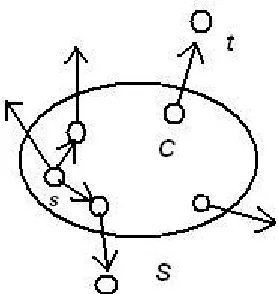
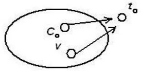
In Dantzig’s algorithm, at first s is assigned a shortest path cost of zero and made the only member of a set S of labeled vertices for which the shortest path costs are known. Then, under the constraint that members c of S are “closer” to

[image:52.612.255.394.390.537.2]

s than nonmembers u, that is, L(s, c) ≤ L(s, u), the set S is expanded until all vertices have been labeled. The expansion process of the solution set is shown in Figure 12.

Figure 12: Solution set expansion process

The above algorithm maintains a candidate edge (c, t) for each vertex c in S.

(53)

vertices still outside S to make the expansion of S computationally easy. If a candidate’s endpoint t is outside the current S the candidate is considered as a useful candidate and useless otherwise. Dantzig’s algorithm requires all candidates to be useful. To meet this requirement the candidate for a vertex c

is selected by scanning the sorted list of edges out of c in increasing cost order until a useful edge (c, t) is found. When a useful edge (c, t) is found we are guaranteed that t is the closest (by a single edge) vertex to c and c ∉ S. Vector

d maintains shortest path costs for vertices that are already labeled, that is

c∈S, d[c] = L(s, c). The edge cost from c to t is given by c(c, t) and the path cost via vertex c to candidate t is given by the candidate weight d[c] + c(c, t).

Vertex t might also be the candidate of other already labeled vertices v∈S as in Figure 13. Each time it is a candidate there will be some weight d[v] + c(v, t) associated with its candidacy. There will be in total |S| candidates, with endpoints scattered amongst the n – |S| unlabelled vertices∉S.

(54)

[image:54.612.261.406.350.423.2]

At each stage of the algorithm the endpoint of the least weight candidate is added to S. If c0 is a vertex such that the candidate weight d[c0] + c(c0, t0) is minimum over all labeled vertices c, then t0 can be included in S and given a shortest path cost d[t0] of d[c0] + c(c0, t0). Then an onward candidate for t0 is added to the set of candidates, the candidates for vertices that have become useless are revised (including that of c0), and the process repeats and stops when |S| = n. Figure 14 shows an intermediate stage of the expansion of solution set S.

Figure 14: Intermediate stage of solution set expansion process

Initially the source s is made the only member of S, d[s] is set to zero, and the candidate for s is the shortest edge out of s.

3.3.3 Analysis of Dantzig’s APSP Problem Algorithm

(55)

candidates to decide whether or not they remain useful. Thus total effort is O(j2). When j = n, this is O(n2).

The other component that contributes to the running time is the effort spent scanning edge lists looking for useful edges. As each edge of the graph will be examined no more than once, the effort required for this is O(n2). Thus the total time for a single source problem becomes O(n2). And the total time for the n single source problems becomes O(n3). The time for sorting, O(n2 log n) is absorbed within the main complexity.

3.3.4 Spira’s APSP Problem Algorithm

Spira [11] also developed an algorithm for Single Source Shortest Path (SSSP) Problem in which an all pairs solution is found by first sorting all of the edge lists of the graph into ascending cost order, and then solving the n single source problems. The algorithm is as follows:

________________________________________ Algorithm 8: Spira’s APSP Problem Algorithm

1: for s = 1 to n do Single_Source(s); 2: procedure Single_Source(s); 3: S := {s}; d[s] := 0;

6: Spira_expand_S(n) 7: end {Single_Source}; 8:

(56)

10: while |S| < limit do begin

11: let (c0, t0) be the candidate of least weight; 12: if t0 is not in S then begin

13: S := S ∪+ {t0};

14: d[t0] := d[c0] + c(c0, t0); 15: if |S| = limit then break;

16: add to the set of candidates the shortest edge from t0; 17: end if;

18: replace (c0, t0) in the set of candidates by the next shortest 19: edge from c0;

20: end while;

21: end {Spira_expand_S}; 22: end for; //end of s

________________________________________

3.3.5 Description of Spira’s APSP Problem Algorithm

Spira’s n single source problems algorithm is quite similar to that of Dantzig. The main difference between these two algorithms is that Spira incorporated a weak candidacy rule and relaxed the strong candidacy rule that requires all candidates to be useful. The weak candidacy rule enforces that all candidate edges (c, t) be such that c(c, t) ≤ c(c, u) for all unlabeled vertices u. The main motivation behind this weak candidacy rule is that the expensive scanning of adjacency lists could be reduced. Note that in Dantzig, t itself must be outside

(57)

3.3.6 Analysis of Spira’s APSP Problem Algorithm

Spira introduced the cost of an increased number of candidates that must be examined during the labeling process by cutting the time spent scanning adjacency lists looking for useful edges. Spira makes an important probabilistic assumption, called endpoint independence that the minimal cost candidate falls on each of the vertices with equal probability. Using lemma 2, the total expected number of drawings of candidates will be O(n log n) until we draw all candidates at least once. Each drawing would cost us O(log n) time for the corresponding tree manipulation, thus the total effort to solve 1 single source problem is on average O(n log2 n). And the total effort to solve the n single source problems becomes O(n2 log2 n).

3.3.7 MT’s APSP Problem Algorithm

Moffat and Takaoka [3] further developed an algorithm which is based on Dantzig’s and Spira’s APSP Problem algorithms and famously known as MT algorithm. They identified a critical point until which Dantzig’s APSP Problem algorithm is used for labeling vertices. After the critical point Spira’s APSP Problem algorithm is used for the labeling on a subset of edges.

(58)

2: procedure Fast_Single_Source(s); 3: S := {s}; d[s] := 0;

6: Dantzig_expand_S(n – n/log n); 7: U := V – S;

8: Spira_expand_S(n), using only the U-edges 9: end {Fast_Single_Source};

10: end for; //end of s

______________________________________

3.3.8 Description of MT’s APSP Problem Algorithm

MT algorithm is a mixture of Dantzig’s and Spira’s algorithms where these algorithms are slightly modified. MT algorithm can be divided into two phases. The first phase corresponds to Dantzig’s algorithm where binary heap is used for the priority queue. This phase is used to label vertices until the critical point is reached, that is when |S| = n – n/log n. Dantzig incorporated the strong candidacy rule. The complexity of this algorithm consists of two components. One is the effort required to label the minimal weight candidate and to replace candidates that become useless. The other one is the effort required to scan for useful edges. The second phase after the critical point corresponds to Spira’s algorithm. This is used for labeling the last n/log n

(59)

useful. Moffat and Takaoka introduced the concept of set U and U-edge. U is defined as the set of unlabeled vertices after the critical point. Also an edge is called U-edge if it connects to a vertex in the set U. These are depicted in the following figure.

|S| = n -

n n

log |U| =

n n

log

[image:59.612.148.491.236.404.2]

U-edge

Figure 15: Visualizing set S, U and U-edge

To improve the efficiency of Spira’s algorithm, Moffat and Takaoka made an important modification to procedure Spira_expand_S. Due to this modification the next shortest edge is not chosen as the new candidate, instead the next shortest U-edge is chosen as the new candidate.

3.3.9 Analysis of MT’s APSP Problem Algorithm

(60)

each of the n – j unlabeled vertices has the equal probability to be chosen as

next candidate. Then we can expect that 1 +

j n

j

− −1

candidates will need to be

taken care of as they becomes useless in each iteration of the while loop of Dantzig_expand_S because by definition the root of the heap will become useless always. And each of the remaining j –1 candidates will become useless

with probability p =

j n−

1

. It be can shown that the useless candidates can be

replaced in O(

j n

j

− + log j ) time on average although we omit details. This expression is O(n log n) only when j ≤ n – n/log n and this is how the critical point was chosen. The expansion of S from 1 element to n – n/log n elements will require O(n log n) expected time.

Now we focus on the scanning effort for useful edges. When |S| = n – n/log n

(61)

Each heap operation in Spira_expand_S requires O(log n) time. Also the edge scanning effort is O(log n) time. One of these two efforts will be absorbed into another. Thus total effort required for a candidate replacement is O(log n) time. Thus each iteration of Spira_expand_S will require O(log n) time. After the critical point there are |U| = n/log n vertices that need to be labeled. As each candidate is a random member of the set U the expected number of while loop iterations required before all the members of set U gets labeled is (n/log

n) ln (n/log n) (using Lemma 2) which is bounded by O(n). Thus the total expected time to label the set U will be O(n log n).

3.4 Modified MT Algorithm as Fast DMM

Takaoka [1] modified MT algorithm and used APSP Problem as a fast engine for DMM. In this section we describe this algorithm in details.

_______________________________ Algorithm 10: Fast DMM Algorithm

1: Sort n rows of B and let the sorted list of indices be list [1], ..., list[n]; 2: Let V = {1……..n};

3: for i := 1 to n do begin 4: for k := 1 to n do begin 5: cand[k] := first of list[k]; 6: d[k] := a[i, k] + b[k, cand[k]]; 7: end for; //end of k

8: Organize set V into a priority queue with keys d[1],……,d[n]; 9: Let the solution set S be empty;

10: /* Phase 1: Before the critical point */ 11: while |S| ≤ n – n/log n do begin

(62)

13: Put cand[v] into S; 14: c[i, cand[v]] := d[v];

15: Let W = {w | cand[w] = cand[v]}; 16: for w in W do

17: while cand[w] is in S do cand[w] := next of list[w]; 18: end for; //end of w

19: Reorganize the queue for W with the new keys d[w] = a[i, w] + b[w, 20: cand[w]];

21: end while; 22: U := S;

23: /* Phase 2: After the critical point */ 24: while |S| < n do begin

25: Find v with the minimum key from the queue; 26: if cand[v] is not in S then begin

27: Put cand[v] into S; 28: c[v, cand[v]] := d[v];

29: Let W = {w | cand[w] = cand[v]}; 30: end else W = {v};

31: for w in W do

32: cand[w] := next of list[w];

33: while cand[w] is in U do cand[w] := next of list[w]; 34: end for; //end of w

37: end while; 38: end for; //end of i

_________________________________

3.4.1 Description of Fast DMM Algorithm

Suppose we are given two distance matrices A = [ai,j] and B = [bi,j]. The main objective of DMM is to compute the distance product C of A and B. That is C

= AB. In this description of the algorithm, suffices are represented by brackets. At first rows of B need to be sorted in increasing order. Then we solve the n

(63)

list[k]. We solve the single source problem first and repeat it n times for n

[image:63.612.212.443.258.472.2]

different sources. The endpoint independence is assumed on the lists list[k] using Lemma 7, that is, when we scan the list, any vertex can appear with equal probability. We consider the 3-layered DAG in Figure 16 in further description of this algorithm.

Figure 16: 3-layered DAG of two (n, n) matrices

(64)

inserted into the solution set S. list[v] is scanned to get a clean candidate for v

so that cand[v] points to a vertex which is outside the current solution set S. Then v is inserted back to the queue with the new key value. Every time the solution set is expanded by one, we scan the lists for other w such that cand[w] = cand[v] and construct the set W. For each w∈W we forward the corresponding pointer to the next candidate in the list to make their candidates

cand[w] clean. The key values are changed accordingly and we reorganize the queue according to new key values. This expansion process of the solution set stops at the critical point where |S| = n – n/ log n. We consider U to be the solution set at this stage and U remains unchanged from this point onwards. After the critical point, solution set is further expanded to n in the same way to label rest of the n/log n candidates which are outside U.

3.4.2 Analysis of Fast DMM Algorithm

Analysis of Fast DMM, not surprisingly, should be quite similar to that of MT. First we focus on heap operations. If a binary heap is used for the priority queue, and the reorganization of the heap is done for W in a bottom-up fashion then the expected time for reorganization can be shown to be O(n /(n – j) + log

n), when |S| = j. This expression is bounded by O(log n) when |S| n – n/ log

n. Thus the effort requires for reorganization of the queue in phase 1 is O(n log

n) in total.

(65)

Using Lemma 2, we can establish the fact that after the critical point the expected number of unsuccessful trials before we get |S| = n is (n/log n) ln (n/log n). This is bounded by O(n). The expected size of W in phase 2 is O(log

n) when S is expanded, and 1 when it is not expanded. The queue reorganization is done differently in phase 2 by performing increase-key separately for each w, spending O(log n) time per cand(w). From these facts, the expected time for the queue reorganization in phase 2 can be shown to be

O(

n n

log × log 2

n) = O(n log n).

|U| =

n n

log |S| = n -

n n

log

Figure 17: Intermediate stage of set W

(66)

3.5 Analysis of MSP (Algorithm 6) based on Fast DMM

We assume m and n are each a power of 2, and m ≤ n. By chopping the array into squares we can consider the case where m = n. Let T(n) be the time to analyze an array of size (n, n). Algorithm 6 splits the array first vertically and then horizontally. We multiply (n, n/2) and (n/2, n) matrices by 4 multiplications of size (n/2, n/2) and analyze the number of comparisons. Let

M(n) be the time for multiplying two (n/2, n/2) matrices which is equal to O(n2

log n) as this is the expected time for the n single source problems by Fast DMM. Thus we can establish the following lemma, recurrence and theorem.

3.5.1 Lemma 8

If M(n) = O(n2 log n) then M(n) satisfies the following condition:

M(n) (4 + 4/ log ≥ n)M(n/2)

Proof:

M(n) = n2 log n

= 4

2

2⎟⎠ ⎞ ⎜ ⎝ ⎛n

log ⎟

⎠ ⎞ ⎜ ⎝ ⎛ 2 . 2 n = 4 2

2⎟⎠ ⎞ ⎜ ⎝

⎛n _⎟

⎠ ⎞ ⎜ ⎝ ⎛ + 2 log 1 n = 4 2

(67)

= ⎟ ⎟ ⎟ ⎟ ⎠ ⎞ ⎜ ⎜ ⎜ ⎜ ⎝ ⎛ + 2 log 4 4

n M ⎟_⎠

⎞ ⎜ ⎝ ⎛ 2 n

> _⎟⎟

⎠ ⎞ ⎜⎜ ⎝ ⎛ + n log 4

4 M ⎟

⎠ ⎞ ⎜ ⎝ ⎛ 2 n

Thus M(n) satisfies the condition.

3.5.2 Recurrence 1

Let T1, T2,.….., TN be the times to compute DMMs of different sizes in the Algorithm 6. Then by ignoring some overhead time between DMMs, the expected value E[T] of the total time T becomes

E[T] = E[T1 + T2 +.…..+ TN]

= E[T1] + E[T2] +.…..+ E[TN]

= E[E[T1 | T2, T3,.….., TN]] + E[E[T2 | T1, T3, .….., TN]] +.…..+ E[E[TN |

T1, T2,.….., TN-1]]

From the theorem of total expectation, we have E[E[X|Y]] = E[X] where X |Y is the conditional random variable of X conditioned by Y. So we can write

(68)

In the above, expectation operators go over the sample space of T1, T2,.….., TN.

Thus we can establish the following recurrence where total expected time is expressed as the sum of the expected times of algorithmic components.

T(1) = 0, T(n) = 4T(n/2) + 12M(n)

M(n) = O(n2 log n)

3.5.3 Theorem 1

Suppose M(n) = O(n2 log n) and M(n) satisfies the condition M(n) (4 + 4/ log n)M(n/2). Then the above T(n) satisfies the following:

≥

T(n) ≤ 12(1 + log n)M(n)

Proof:

Basis step: Theorem 1 holds for T(1) from the algorithm.

Inductive step:

T(n) = 4T(n/2) + 12M(n)

= ) 12 ( )

2 ( ) 2 log 1 ( 12

(69)

≤ ( ) 12 ( ) log 4 4 2 log 1

48 M n M n

n n + × + + ×

= ( ) 12 ( )

) log 1 1 ( 4 2 log log 1

48 M n M n

n

n _× ₊

+ − +

×

= ( ) 12 ( )

log 1 log 1 log 1

12 M n M n

n n n + × + − + ×

= ( ) 12 ( )

log 1 log

log

12 M n M n

n n n + × + ×

= ( ) 12 ( )

1 log log 12 2 n M n M n

n _× ₊

+

×

= ( ) 12 ( )

1 log log log log 12 2 n M n M n n n

n _× ₊

+ − +

×

= ( ) 12 ( )

1 log log ) 1 (log log

12 M n M n

n n n n + × + − + ×

= ( ) 12 ( )

1 log

log log

12 M n M n

n n

n _⎟⎟× +

(70)

12 log ≤ n M(n) + 12M(n)

= 12M(n) (log n + 1) = 12(1 + log n)M(n) (proved)

Thus the total complexity of Algorithm 6 based on Fast DMM becomes O(n2

log2 n). Because an extra log n effort is required on top of the Fast DMM complexity due to the recursion in Algorithm 6.

3.6 K-MSP Algorithm

(71)

Chapter 4 K

-Tuple Approach

DMM can be generalized as K-DMM as we already explained this in Chapter 2 (Sec 2.6). In this chapter we modify Takaoka’s Fast DMM based on MT algorithm where APSP Problem is incorporated as a fast engine for DMM. In the following algorithm, we extend the Single Source Shortest Path Problem to the Single Source K Shortest Paths Problem and establish Fast K-DMM algorithm by incorporating n such problems.

In the following algorithm we have the outermost loop by r. Data structure T is used to identify edges already consumed in shortest paths for previous r. T can be implemented as a 2D array where at every location we maintain a set of second layer vertices of the 3-layered DAG through which a path has been established for a given pair of source and destination.

4.1 New Fast K-DMM Algorithm

_________________________________ Algorithm 11: Fast K-DMM Algorithm

1: Sort n rows of B and let the sorted list of indices be list[1], ...,list[n] 2: Let V = {1……..n};

3: Let the data structure T be empty; 4: for r := 1 to K do begin

(72)

6: for k := 1 to n do begin 7: cand[k] := first of list [k];

8: while k is found in the set at T[i, cand[k]] location do begin 9: cand[k] := next of list[k];

10: if end of list is reached then begin

11: cand[k] := n + 1; //(n + 1)th column of b holds 11: // a positive infinite value 999

12: end if; 13: end while;

14: d[k] := a[i, k] + b[k, cand[k]]; 15: end for; //end of k

16: Organize set V into a priority queue with keys d[1],……, d[n]; 17: Let the solution set S be empty;

18: /* Phase 1: Before the critical point */ 19: while |S| ≤ n – n/ log n do begin

20: find v with the minimum key from the queue; 21: Put cand[v] into S;

22: c[r, i, cand[v]] := d[v];

23: Put v in the set at T[i, cand[v]] location; 24: Let W = {w | cand[w] = cand[v]};

25: for w in W do begin

26: while cand[w] is in S ORw is found in the set at T[i, cand[w]] 27: location do begin

30: cand[w] := n + 1; //(n + 1)th column of b holds 31: // a positive infinite value 999 32: end if;

33: end while; 34: end for; // end of w

37: end while; 38: U := S;

39: /* Phase 2: After the critical point */ 40: while |S| < n do begin

41: find v with the minimum key from the queue; 42: if cand[v] is not in S then begin

43: Put cand[v] into S; 44: c[r, i, cand[v]] := d[v];

(73)

46: Let W = {w | cand[w] = cand[v]}; 47: end else W = {v};

48: for w in W do begin

50: while cand[w] is in U OR w is found in the set at T[i, cand[w]] 51: location do begin

54: cand[w] := n + 1 //(n + 1)th column of b holds 55: // a positive infinite value 999 56: end if;

57: end while; 58: end for // end of w

61: end while; 62: end for; // end of i

63: end for;// end of r

_________________________________

4.2 Description of New Fast K-DMM Algorithm

The new Fast K-DMM algorithm is primarily based on Fast DMM algorithm (Algorithm 10). Some of the descriptions of Fast K-DMM algorithm should be quite similar to that of Fast DMM algorithm. So we omit similar descriptions here for Fast K-DMM algorithm that we’ve already discussed for Fast DMM algorithm and only focus on the new enhancements that we have made into Fast K-DMM algorithm.

(74)

arrays a[1..n, 1..n] and b[1..n, 1..n + 1]. Note that each row of b has n + 1 columns. This is because we need an extra position in each row to store a positive infinite value.

In this description we consider the 3-layered DAG in Figure 16. The variable r

in the outermost for loop runs from 1 to K which determines the number of shortest paths for the n single source problems. As there are at most n numbers of different paths from a source to a destination, K must be n. Also we put 999 as a positive infinite value (as we assume all the numbers that appear in the given (m, n) array are between 1 and 100) at the (n + 1)th column of all the rows of array b. To explain this let’s consider the following situation.

≤

(75)

1)th position as the candidate of k which in return will access the (n + 1)th column of the kth row where we have 999 as a positive infinite value.

We also maintain a data structure T to manage second layer vertices through which paths have been already established. We call second layer vertex as via

vertex. In the next section we explain in details how we implement data

structure T.

4.2.1 Description of Data Structure T

Average case analysis of algorithms for the maximum subarray problem

Examining Committee:

Abstract

Acknowledgments

Table of Contents

List of Figures

List of Tables

Chapter 1

Introduction

10 22 6 28

1 6 35 27

6 24 27 14

5 54 3 4

Sales[Row][Col]

A

Ag

ge

e

G

G

r

r

o

o

up

u

p

In

I

nc

co

om

me

e

L

Le

ev

ve

el

l

Sales[Row][Col]

A

A

g

g

e

e

G

G

r

r

o

o

u

u

p

p

I

I

n

n

c

c

o

o

m

m

e

e

L

L

e

e

v

v

e

e

l

l

-7 5 -11 11