A study of the non linear dynamics of vortex flows by numerical methods

University of Warwick institutional repository:

http://go.warwick.ac.uk/wrap

A Thesis Submitted for the Degree of PhD at the University of Warwick

http://go.warwick.ac.uk/wrap/74486

This thesis is made available online and is protected by original copyright.

Please scroll down to view the document itself.

A study of

the non-linear dynamics of vortex f'Lows by numer-i cnL methods

I

by

Jes Peter Christiansen

A dissertation subnri tted to the University of Har.rick for

admission to the degree of Doctor of Philosophy

BEST COpy

.

, .AVAILABLE

, Variable print quality

IvD};HORAHDUH

This dissertation is submitte<l to the Universi ty of iVarilick in support of

r~ application for admission to the deGree of Doctor of Philosophy. It contains an account of my own troz-k per rcrmed at Culham Laboratory, Abingdon

and at the School of Physics of the University of "llarwick in the period

September

1969

to January

1972

under the general supervision of

Doctor K.V. Roberts of Culham Laboratory and Doctor G. RovLands of the

University of HarvTick. no part of this dissertation has been used

previously in a decree thesis submitted to this or any other University.

T'ile wor'k described in this thesis is the result of my own independent

research except wher-e specifically acknowLedged in the text.

J. P. Christiansen

'.,_CKIIOHLEDGEl,1ElITS

--'l'he author ,·rishes to expreus his de ep gratitudc to Dr K V Roberts and Dr G Rowlands for their cO::ltinueu interest anu. encouragement

through-out the course of this iwrk. I wish espec ial.Ly to thank Dr J B Taylor and

Dr NJ Zabusky for their cooperation and helpful assistance. I would. also like to thank all those members of the Computational Physics Group and

Applied l-lathematics Group at Culham Laboratory I who have been available

for discussions. furtherMore, I wou.l.d like to t.hanl; the computing staff

at Culhwl Laborato~J for helpful assistance.

I gratefully aclmov'Ledge the financial support provic1ed 'by the

United Kinr,dom At.omi,c Energy Authorit:r and by m.yfather L.Clu:istianscn.

Finally, I wish to thank I'll's H J3 Penge.LLy for her s)dll und pat ieuce

in typing this thesis.

ABS'rrv\CT

The subject of motions in two-dimensional ideal fluids is treated by

numerical methods and the results given an interpretation based on

theories as well as numerical experiments. Phenomena in ideal fluids

have relevance to flows in realistic fluids when the flow speeds encoun-. .

tered are much smaller tha~ the speed of sound and when dissipative

mechanisms playa negligible role. The restriction to consider only

motions of two dimensions is established and the resulting mathematical

description yields a classical formalism. In terms of the scalar vorticity

the motion of a two-dimensional ideal fluid can be interpreted by the flOyT

in phase space of a classical phase fluid. The scalar stream function

acts as a Hamiltonian for a system "Those phase space corresponds to real

space. TriO models 1-lithrespectively an infinite and a finite number of

degrees of freedom,are used to picture the evolution with time of the

vor-ticity distribution. The former model, the field model, is used in

analytic studies, and the latter model, the particle model, is employed in

the numerical approach. The field model is reviewed as an introduction to the SUbject. The pe.rticle model is fitted into a numerical scheme that

forms the basis of a computer simUlation code

VORTEX.

This n~~erical

scheme is presented in detail and made the subject of a numerical analysis.

Controlled numerical experiments are carried out to establish possible

inaccuracies of the scheme and the sources of these inaccuracies are

\

revealed by means of the results from the numerical analysis. The general work of preparing controlled nUDlerical experiments is briefly

mentioned and by recording the experience from several numerical

experi-ments the quality of these can be assessed. Results of several numerical

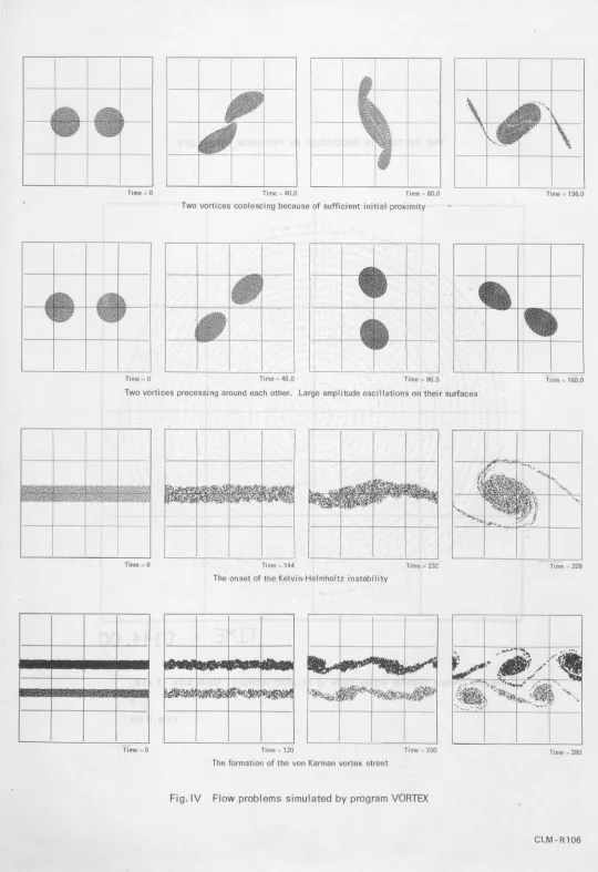
experiments are then presented. The problem of two-dimensional turbulence

is tackled by a precursory study of the interaction between finite area

vorticity regions. An analytic calculation is made to support the

numerical simulationR which demonstrate the non-linear aspects of vortex

interactions: fusion of strongly interacting vortices of the se~e sign

and large amplitude oscillations in the flm'l from two vortices of opposite

sign. The numerical experiments that follow, treat the stability and long

time evolution of laminar 'Takes, and heuristic comparisons are made vdth wind tunnel experiments that minimise three-dimensional effects. A model

of four finite-sized vortices

is

used to study the stability of von Kar.m~

vortex streets. Comparisons with theory are made and the results show

fusion of like-signed vo~tex regions as well as fission of a vortex

in

the presence of other vortices. The final stlldy comprises numerical

experi-ments with a model approximating vortex flmm in jeta. It is concluded

that much insight can be gained by using relatively simple flmT models

combined ''litha suitable numerical scheme in order to understand the

Publications

Various aspects of the work described in this thesis have been pub Li shed ,

or are in. the course of ]!ublication in the scientific literature. Hith

reference to the chapters of this thesis the relevant pubLi cat ions arc:

CHAPTER1 CHRISTIAHSEN,J P .and ROBER1'S,K V , 1969. Paper l}O in

the ProcecuinGs of the Computational Physics Conference

at Cu.Iham Laboratory, <Tuly 1969. Available from HNGO.

ClIAPTEH2 CHRISTIAnSEH. J P and HOCKlmY,R i-T , 1971.

Comp ,Phys •Comn ,

,g,.

127.

CIIRISTlAiISEH. J P and HOCK1JEY,R)v , 19'(1.

Comp ,Phys •Coram.

,g"

139.

CHRISTIANSr:H,.T,p • 1971. numerical simula.tion of

hydro-dynamics by the method of point vortices. illCJ\EA Cu.Iham

Report CLH-P282 submitted for publication in Journal of

COTn!,utational Physics.

CHRISTIAHSEH,J P and ROBERTS,

K

V , 1969. numerical

simulation techniques applied to incompressible

hydro-dynamic flows. 3rd fulnual Conference on Plasma Simulation

a·t Stanford Uni vers i ty. September 1969.

ClffiISTIAUSEH. J ..p and ROBERTS,K V , 1969. Paper 51 in the Proceedings of the Computational Physics Conference

at Cu.lham Laboratory, July 1969. Available from

Ill-mo.

ROBERTS,K V and CHHISTIAlISEN.JP. 1972. Topics in

Computational Fluid Hechanics. COr.l.p.I'hys.Corron.

1.

Sullpl.

CHAPTER l~ :

CHAPTER

5

APPENDIX

CHRIGTIAlISEHt J P and ROIICRTSt K V , 1970. The

non-linear deveLopmerrt of modes on the surf'ace of circular

vortices. Conference Dieest, Computational Physics,

The Institute of Physics and the Physical Society, London.

CHRISTIAnSEN", J

P

and

HOBERTS, K

V , 1971. Simulation of

hydrodynamic systems oscillatine "ith laree amplitudes

arowld stationary equilibriun states. 5th Annual

Confer-ence on Plasma Simulation at University of Iowa, Nov.1971.

CHRISTI.ANSEN, J P and ZABUSKY, N J , 1972. Instability,

fission and fusion of asymmetric vortex structures.

UKAEA Culham Report CJ1.1-P30G. Submitted for publication in

Journal of Fluid Mechanics.

CIllISTIAHSEH, JP, 1970. VORTEX, a two-dimensional

hydr-dynamics eimul.ation code. mWi:A Research Report CUI-RI06.

MEHORANDID1 ACKNOWLEDGEEEWL'S ABSTRACT PUBLICATIONS INTRODUCTION CHAPTER 1: 1.1 1.2

1.3

1.4

1.5

CHAPTER 2: 2.1 2.2

2.3

2.4

2.5

2.6

2.7

2.8

2.9

2.10 COHTEnTS

Approach to Co~putational Physics.

Ilydr-odynami.cs and Computational Physics. Research carried out.

IDEAL FLUIDS OF T\iO DIMENSIOnS

Haterial. kinematical and dynamical preliminaries.

Rotational and irrotational motions. Definition of vorticity.

Two-dimensional motions. Hamiltonian equations.

Classical phase fluids and their invariants of motion.

The area fWlctions. The constant vorticity model.

nll-mRICAL snruJ..ATIOn OF r·10TIONS IH 2D IDEAL FLUIDS

Point vortices.

A numerical scheme for the motion of point vortices.

The effects of the finite difference formulation.

The square-shaped boundary.

~~e effect of the discretization of time.

Effects introduced by the mesh. Properties of the test system.

The set-up for numerical simulation.

Results of the ·numerical experiments.

Advanta~es and deficiencies o~ a particle approach.

CHAPTER 3: CHAPTER

4:

4.1

4.2

4.3

4.4

4.5

4.6

4.7

4.8

4.9

4.10

CHAPTER

5:

5·1

5.2

5·3

5.4

5.5

5.6

5.7

GElIERAL DISCUSSIOH OF Il-1PLEr,lEHTING nUMERICAL EXPERIHEIITS

~ne computer codes.

General data for numerical experiments. Units.

Initialization procedures.

Boundary conditions.

The quality of the numerical experinents.

THE INTERACTIOn BE'.r\VEEN VOHTICES

or

FIIUTE SIZE

Introduction.

Rankine's combined vortex.

The intera~tion between vortices.

'!'heweak interaction between t'\-1Ovortices.

The enerGY balance.

A brief introduction to the numerical experiments~ The interaction between a Rru1kine vortex and a point vortex.

Numerical experiments on we~~er interactions.

Numerical experiments 011 strong interactions.

Short summary ,

STABILI'rY PROPERTIES OF VORTEX CONFIGURATIONS MODELLING LA!1IUAR llAKES AnD NOZZLE FLOI-TS

Introduction and epitome of numerical experiments.

Comments on previous ru1alytical work.

Laminar 'Take with a triangular velocity profile.

Laminar wake vdth a trapezoidal velocity profile. Stable asymmeta-Lc vortex contti.gurat.Lons ,

Unstable asyw~etric vortex streets.

Collinear asymmetric vortex streets - standinB waves.

Approximated vortex flows arising from jets.

CO:WLUSIOU

BIBLIOGRAPHY

APPENDIX

page

138

141

Tables A.l - A.3

VORTEX, a t"To-dimensional hydrodynamics simulation code.

INTTIODUCTION

The introduction to this thesis outlines our approach to Computat Lonul, Physics. The combination of llydr-odynami ca and Couputational Physics is

treated in a short r-evi ev of previous relevant work. .An account of the

research carried out is given as a survey of the work presented in each

chapter.

Approach to Computational Physics

The advent of hiGh-speed computers has over the last decade exerted an

influence on practically eve'r'Jscience. The almost explosion-like evolution

of computer technology has made it difficult to forecast llhat future role

conputers will play. In some areas of experimental sciences analogue

com-puters have replaced human beings, whiLst in other areas a digital computer merely acts as a fast slide rule or £)ra1'hplotter. It is Quite clear that

a variety of views on the significance of computers must exist amongst the people who design them, use them and those whose work can be conput er-i.sed ,

He shall not attempt to promote any of these views, but only try to briefly

establish the areas covered by Computational Physics.

By definition we think of Computational Physics as the discipline in

which the elementary operations inherited from Applied Mat.hematLcs are

processed by computing mach i.nery to produce results of a physics

calcula-tion. At its inception this discipline was conceptually identical to

Applied Mathematics. Today, some 10-15 years later, Computational Physics

is in the process of being established as a self-contained discipline.

Although several classical areas of physics are involved in one way or

another, it is generally accepted that Computational Physics mainly

inter-acts with the following branches of science:

\

1. Theoretical Physics and Hathematics

2. Experimental Physics

3. Applied Hat.heraat.Lcsand Numerical Analysis

4.

The general science of computers.

1,1anyopinions exist as to how emphasis should be placed on each of these

areas. The rrull(of priorities given to the work in this thesis follows

from the list above and is put "in manifesto" by the division of the

research work into distinctly separate chapters. The time and effort spent

-in each of these four areas are however not proportionally represented in this thesis, as it would change the raQKof priorities Given above. It is the opinion of the author that at present too much time and effort are often spcnt in the area of coinput i.ng science, the handline of computers and the I-lriting of compuber progr-ams, Hot surprisinclJr one finds in the

scientific communitya vidoapr'ead lack of distinction between computing science and computational physics. It as thc author's hope that the work presented in this thesis will do justice to making that distinction clear. Hydrodynamicsand Corwutu,tional Physics

Hydrodynamicsis one of the oldest disciplines in modern physics, yet with a rather peculiar history. To r evi.ev its history is beyond the scope of this thesis and therefore only features of relevance to the present vork 'fill be mentioned. - The initial interest in hydrodynamics arose from

attempts to describe thc dynamics of continuous med.ia , e.G. fluids. The present interest establishes itself throuGh many disciplines associated ,·lith hydrodynamicse "The deveLopmerrtof aircraft has caused an interest in

aerodynamics and hydraulics. The exploration of the solar system and advances made in astrophysics have 'developed magneto-hydrodynamics. nuclear fusion research has pushed forward theories in plasma phYBics. The con-struction of large ships and submar:i.neshas intensified experimental hydrodynar.lic studies".

ftmda-ised model has been superseded by more realistic and also more complicated mentally exhibit dynwlical properties described by the partial differential

equations of hydrodyno.mics. These equations were formulated in

1760

by

Euler with applications to a simple fluid model. Since then Euler's

ideal-models. These latter models introduce concepts like compressibility of a

fluid, viscous forces, electromaeneto-dynamic forces, oblique stresses etc.

All these concepts serve to account for the complexity of the internal fluid

structure; somet~llleseven more than one fluid is being introduced. in a

model. Research on such complex models is often confined to studying the

influence of new features of the internal fluid structure rather than the

ceneral dynamics of the model.

In order to understand the dynamics of fluids it seems reusonaole to

consider first the motions that occur in simple fluids. The present vork

is conceived in the belief that many intricate and perl')lexine fluid motions

can be explained by studies of idealised models. The most ideal model we

can think of consists of a fluid "hose rtll"l.terial(molecular) composition has

no effect whatsoever on any motion into which it can be set. Such a fluid

is called an ideal fluid and it has been the subject, matter of many investi-gations. Hotions in ideal fluids will bear some relationship to flovs in

real fluids when the flow speed encountered are much smaller than the sound

speed and dissipation of energy due to viscous forces can.be neglected • .An

ideal fluid is incompressible such that any disturbance communicated travels

at infinite speed.

An

ideal fluid ~s also inviscid (zero viscosity) and its

density is usually assumed uniform.

Most of the flows occurring in fluids are rotational, e.g. two- or

thre~-dimensional phenomena. This important feature is reflected in Kelvin's

minimum theorem and also in a demonstration by Kirchoff and Kelvin stating that

ii-rotational f'Lovs are in general ir1possible (see Lamb, 1932). The con-ceptual·backbone of rotational motions is centered around the definition of

vorticity, a quantity introduced by d'Alembert and now used by most authors

-in hydrodynamics. The vorticity is a vector deucr-i.bing the instantaneous

rate of rotation in a plane perpenclicular to the vectorial direction.

(The standard sign convention applies). Vortices are finite fluid regions

that poss~ss vorticity and a vortex can be shaped like a rinc;, a twisted

tube, or a cylinder. The motion of the fluid can be described by the

motion of vortices: knovi.ng the vorticity distribution we can determine

the resulting flow· field.

v/hen a motion as strictly two-dimensional then the description in

terms of vorticity of a tlvo-dimensional ideal fluid can be based on a

Hamiltonian formalism, a feature discovered by Kirchoff. The vorticity

becomes a scalar f'uncti.on whose evolution ldth time is governed by

Poisson's and Liouville's equations. The scalar vorticity distribution

behaves as a classical phase space distribution in a tlvo-dimensional phase

space. Such a situation he.sreceived attention from many authors and

various models have been employed to picture the flmT of an Lncompr-eas ibj e phase fluid. 'rhe vortices which are the sources of the flow field are nov

restricted to luove about in a plane and correspond to rectilinear vortices

in

a

three-dimensional flmT. Although the mathem.atical description of

two-dimensional ideal fluids in its classic formalism is attractive to employ

for studies of hydrodynami ccf'Lovs, "loreadmit its inadequacy to represent

more than a highly restricted class of phenomena whose dynanics becomes

degenerate throuch the lack of the third space dimension.

The various models used to picture the flow of a phase fluid can be

divided into t"t-TOclasses. In the first class the vorticity distribution is

represented as a truly continuous function. In the second class the

vor-ticity distribution is considered to arise from a finite number of point

vortices which are analogous to point charges in electrostatics or point

masses in gravitational problems. A point vortex can, like a point charge

irroto.tional motion with a singularity at its position. The tlw classes of

models are based on

tvro

descriptions: field model (continuum) and

action-at-a-distance model (point vortices).

A Tiloaelof the first class, called "the constant vorticity model" is

of particular interest to our work. In this model the vorticity takes

constant values diffel'ent from zero an areas confined by contours. If these contours are closed we thinJ~ of the area as being a vortex. The constont vorticity model has been used in studies by Kirchoff, Kelvin,

Love, Hill and later by Proudman and Lamb. Because of the non-linearity

of the hydr-odynarai c cquati.on only special systems involving sirap.l,econtours are treated. Host of this worle is reviewed in the books of Bassett

(1888)

and Lamb (1932).

The point vortex model originally introduced by Kirchoff is rigorously

analysed by Lin (1943). It vias used by von Karman (1911) in

a

study of the stability of vortex streets (parallel arrays of oppositely-signed point

vortices). Von K8.rn8.n'sstudy was extended by Rosenhead (1929 &: 1930) and is also treated in the book by Kochin, KibeI &: Roze (1961+). The most important work on the point vortex model is presented in a paper by

Onsager (19h9) who attempts to develop a theory of the statistical mechan-ics of ensembles of point vortices. This paper has been followed up by a

study by Morikawa (1960) with applications to meteorology.

With the advent of computers it is possible to treat previously

insOLvable problems, e.g. non-linear proble~s, by applying suitable nmnerical

methods to approximate the partial differential equations. A nerTsubj ect ,

Computational Fluid l1echanics, has grown from the efforts made to

under-stand the non-linear dynamics of fluid flows. A review of these efforts is

given in the form of an annotated bibliography by Har-Low(1970).

Recent work in the field of Computational Fluid Hechru1ics comprises a

-study by Abernathy & Kronauer (1962) of the formation of the von Karman vortex street. Lately this study has been repeated by Kadomaev &

ICostomarov (1972). Both studies employed the point vortex model treating

the point-point interaction by an exact method~ however for a small number

(~ 50) of point vortices.

The majority of relevant nunlerica1 investigations have been based on

transformations of the partial differential equations into finite

differ-ence forms. In most studies the effects from viscous forces are introuuced

as is the case in the work of Fromm

e;

Harlow (1963), Leith (1969) and Zabusky & Deem (1971). The most intriguing pr-obLem dealt vith is that of turbulence from a t,m-dimensional point of view (Kraichman, 1967) and a

variety of approaches to this problem have been made. A straichtforYrarcl

fini te difference attack on a three-dimensional turbulent flo,.,(for exarnp.Le

through a pipe) can never succeed in pr-acticc when the viscosity is small, as pointed out ·by Emmons (1970). This example serves to illustrate how

Computational Fluid l'-1echanicsand Computational Physics in e;encral are

con-fined to deal with abstr~ct models (dimensionality, eeometry, fluid

proper-ties etc.). Ueverthe1ess 11uc11insiGht and qual.Lt.at Ive undera'tand i.ng of real phenomena can be gained from nuoerical calculations and this leaves

the field of Computational Fluid Hechanics open for innovations of both

numerical 8l1d physical nature. The conclusion reached by most authors in

the field is that much further work remains to be done.

Research carrie,l out

The scope of the work has settled in various forms during the

threc-year period of research. n1C material presented in this thesis represents

approxima.te1y a third of the research period. The remaining material

com-prises the desiGn and testing of computer codes (see Appendix) and the

ised in a paper by the author and J.13. Taylor (1972).

The work began with the development. of a computer code, VORTEXj

capable of s imu'Lating a restricted class of tuo-dimensional floYlS in ideal fluids. Its background, design and operation is presented in a report included as an appendix to this thesis. The operation of the code was carried out on the Cu.lhamLaboratory ICL

KDF9

computer for vlri.ch the VORTEXcode had. been specially deei.gned, The Gra11hical output presented as figures in this thesis was eenerated by a Benson-Lehner 120 microfilm recorder.

-" b" " t"

In chapter 1 vIe set out to descr-Ibe the as as of our iwrk: mo a.onsari

ideal fluids of t'HOdimensions". The concept of vorticity is introduced to demonstrate that the motion of ideal fluids of two dimensions can be pic-tured as the flow in phase space of an incompressible phase fluid. Our description adds no new contributions to the subject; it serves, as a guide to the follQ\oring chapters. In our work we have however aimed.at expanding and elaborating the work of Onsager

(1949).

Because a phase fluid of tIm dimensions is a classical system, one vlould expect to establish a theory of thermodynamic equilibria including

concepts like 'cemperature, entropy etc. \ilien a point vortex model is studied we have a finite number l~ of degrees of freedom such that Gibbs general theory of thermodynamic equilibria applies. If the field model is studied we have a system iofith an infinite number of degr-ees of freedom, but

\

such systems are well-knOlm, the most familiar example being the classical

electromagnetic field. By itself, a classical system with an infinite nmnber of degrees of freedom behaves in a self-consistent way. If we follQ\oIprinciples laid downby Lynden-Bell (1967) it is possible to show even in the limit H ->-,00 that in equilibrium the vorticity distribution,

when the entropy (suitably defined) is maximized, is that given by

-Lynden-Bell. It should then be possible to define the usual thermodynamic

quantities when N -+ co. For a finite H OnsaGer

(1949)

defines

ter.1pera-ture and shovs that it can take positive and negatLve values. Our advances in the case H -+ co end at this point because the area-functions described

at thc end of chapter 1 cnter all the mathematical expressions involved

and we have had no success in det.ermi.ning these functions. 'rhus we have

not found it worthwhile including this study in chapter 1.

Chapter 2 represents a self-contained description of the numerical

method employed to appr-ox.imate the partial differential equations.

Although we aim at studying field models (continuous mode Ls ) we have chosen

to approximate these by a discrete set of point vortices which are then

essentially regarded as particles. The particle model, which has found

extensive use inPlasrna Physics (sec references at the end of chapter 2)

is fitted into a numerical scheme which solvcs the appropriate equations

on a square Cartesian mesh. All physiCal quantities (e.g. vorticity,

velocity field) are then readily calculaJle. In order to understand the

effects arising from the approximations made we perform a series of

con-trolled numerical experinents on the flow induced by a sinG~e circula.r

vortex of finite size (a Hankine vortex). The results from these

experi-ments reveal certain wldesired features of our numerical model and in the

light of a numerical anafysia of this model we explain the sources of the

errors in the results. At the end of the chapter it is concluded that the

numerical approach is suitable for our studies and the limitations on

these is established to some extent. The numerical scheme we describe is

a new scheme and like other schemes it has its advantages and deficiencies.

\'le find that the studies made in the following chapters could not have been

made with any other existing scheme.

Chapter 3 is intended to indicate the considerations that go ahead. of

short as possible, since it wou.Ldexcessively sve.l.Lthe bulk of this thesis

if

all nUJYIericalexperiments perfortlcd were to be described in detail. He outline features that are commonto most of our numerice.Lexper iraent,s and discuss t.he initial vorticity distribution:> and boundary conditions used. 'fa back up the conclusion of chapter 2 we commentin e;eneral on the quality of the nUlIlerical experiments by quoting results from these.

The work.presented in chapter

4

is related to the problem of turbu-lence in ideal fluids of two d.irsensions (ICraichnan,

1967).

To tackle this problem we have initially found it vrorthiYhile studyinG the interaction

properties of systems with tvo fini te-GizcC: vortices. '1'11eintention 01' the stUdy is to establish some features of the large scale Lengt.h behaviour of turbulent motions.

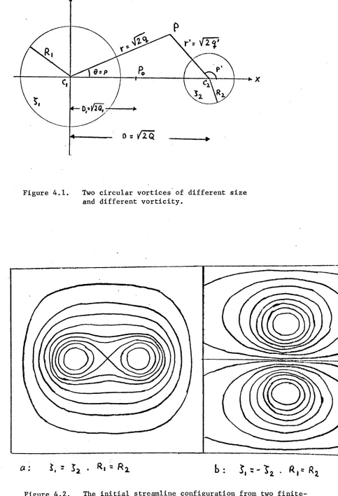
The first part of the chapter covers an analytic ca.l.cuLrrtion of the interaction between two vortices. Such a caLcu.Lati.on applies· to weak interactions over a longer tine-scale or strollG interactions'over a short til:le-scale. The analysis demonstrates that finite-sized vortices undergo a motion as if they were point vortices. Ilovevcr , because they are of finite size their shapes depart from the initial circular shape. The deformation is explained by the pr es ence of surface waves that carry nega-ti v e encr'gy, 'fhe calculation yields formulae for the ampLitudes and

frequencies of these surface wavcs, Because of the erOlyth of surface waves energy is released and made available for the vortices to approach or move aw~r from each other.

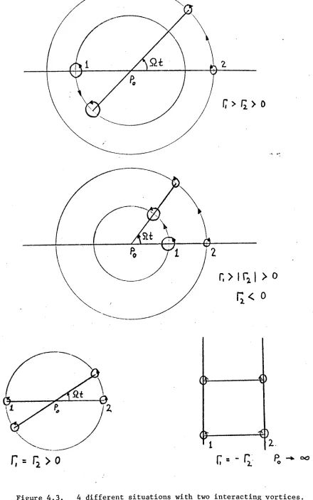
The nUlnerical experiments on vortex interactions arc described in the second part of chapter I!. For experiments on weak interactions ve find aereement llith the theory. For strong interactions we find that like-signed vortices (same ·direction of rotation) approach and fuse together to form a single vortex. Strong interactions between oppositely-signed

-vortices lead to a peculiar dynami,csituation: Lar-geamp.Lit.ude oscillations of the surface waves arc f'ound to £>.creewith theory and an apparent restora-tion of their initial circular shape 1,s estaoLished after one rotation

period of the vortex.

He believe that these non-linear phenomenacan be given an interpreta-tion in terms of the thernodynar.1ic quanti ties mentioned earlier: "At a given energy of a system of 111 vortices a particular number112 of vortex ree;ions ,viII maximize the entropy S(e.c. 8 = 8(n)). The final equilibrium state ,·rith n2 vortices or vortex reGions can be reached, if cuf'f'Lc ierrt free energy (released by the O·o....Tth of negative energy vaves ) a.s made available for the transition ill -+ n2 to occur". This statement Generalizes the

transition 2 -+ 1 observed 1n the numerical experiments of chapter

4.

In

chapter

5

ve observe the transitions

4 -~

3 and

'+

-+ 3 -+ 2 both correspond-. ing to fusion of nearby vortex reeions, but also the transition

h

-+

5

is

found corresJ_:lonuineto the fission of a vortex. Obviously a further stuuy J.n this area is require<1. Ultimately one would like to describe the Ol1set of tW'o-dimensional turbulence in terms of an increase in entropy and to predict whether such an increase is poss i.bLe, Unfortunately our statements about this are as inconclusive as those of Onsuger (19)t9).

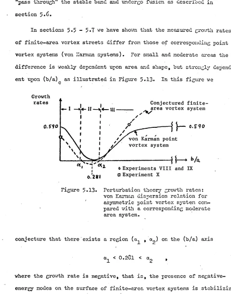
Chapter 5 treats the stability and lone-time evolution of two-dimensional vakes , Humerical experiments on shear unstuble velocity pro-files of laminar f'Lowsare described. The results lead to a study of an \ asynunetric four-vortex finite area system corresponding to a von Karman street of point vortices. The critical parameter of this systen is bla, the initial transverse-to-lonGitudinal separation of vortex centres. At bla ;::0.231 the four-vortex system is stable in agreem.entvTith the

instability are smaller/larGer res:pcctively than that pr eui.ct.ed by the

theory of von Karman. Fusion anrl fission of vortices arc observerl in

these experiments o.nd~TC make heuristic conpar inons with t.hose

t'HO-dimensional t.unnel, experiments that ar e dcs cr ibcd in the becinninG of the

chapter. Finally we look at numerical experi.ncnt.s on a model approx.i-.

matine; the vortex f1m-m f),risinG frO):l jets which cacape nozzles. A

comparison is nade with an analytic nt.udy by llich8.lkc t:: rl'iL'me(19G7). A certain measure of disaGreement be tvoen the gr ovt.h rates of an inst(;J)i1ity

as prcdicte<l by the theory and the e;rm-lth rates measured as cstal)lishcd.

A tentative explanation for this ~s Given.

l~t the end of this thesis we summar-i.ae the "Torl: pr eaerrt cd and we

attempt to draiT conclusions about its future prospects.

-CHAPTEH 1

TI'lO-DHlI:.:lISIOH./".l, IDEAL FLUIDS

An

ideal fluid is an abstraction from a real fluid but if:: considered.

a useful concept from an analytical and computational point of V1.e-W'.

This chapter describes the details of the abstract.ions made. It is shown

that strictly t,w-dimensional motions of ideal f'Lu.ida can be interpreted

,

via the motion in phase space of a classical phase fluid. 'I'his phase

fluid is the part of the ideal fluid which possesses vor:ticity. 'I'he

particular vorticity models used in the resea.rch work are introduced.

1.1, ligterial, kinenc.ticn!, DJJ.d.?-:'1118Jlic8.lprelin:in[lrics

matter d.ealt "ith can be reGurded us continuous in s t.ruct.ure , A motion of

a continuum is taken to be a onc-paranet.er fanily of mappi.ngs of the

COD-ti.nuum on to ot.ner continua. 'I'he par-amct.ex is time t with a continuous domain of variatd on , - 00 < t < "", t

=

0 be i.ng an arbitrary initial instant.

The continuum is occupied. "by a fluid. vhos e mo.Lccul.ar composition remains

invariant vTith tiY1c. A finite set of querrti.ties are assumed. to dcacr i.be the state of the fluid exhaustively. These quantItics are presented as

mathematical I'unct i.ons

l1i

(E.,

t) CivinG the vrrLue of qi o.t time t at a point v1ith coordinates

,.

-

.

The coordinate r is neasured in a coorrrinct.e

-system at rest ana the descr-i.pt.Lon in terrns of '-'. (r_{'oil _,} t) is c a.l.LedEul.er-Lan , An alternative description called Lagr ang.ian expresses Q. as Q.(n(t)) llher€!

~ ~

-~(t) is the coordinate of a point movine with the fluid. In both

dcscrip-tions Yle chronicle the historv of

Q. •

" ~

In order to establish a pattern of histories C01'1JTIOnto f'Lirids of

different molecular composition it s eena natural to consider only properties

commonto all fluids. Loeicall~r there are only tvTO such properties: the

space coordinate r and till1e t. A fluid "'hose history in all possible

circumr;tances can be d.escribed an terms of these tYTOquanti ties as ,.,ell as

properties clerivecl f'r om rand t as called an ideal fluid.

Althour)l the molecular composition of an ideal fluid need not be

specified, its Lnvar-iance uith time i!'lplies that no finite portion of the ideal fluid can be created or destroyed durine any motion.

3

dY

=

d

I~I

,.,hich at time t occupies the spatial volume dv

A volume

3

=

d

lEI

remains

invariant throughout any motion

(ev

=

dv ) which then is called isochoric

(volume preservinG).

A

fluid susceptible of isochoric mo'tions only is

normally caller: an incom)!rcssible fluid. I(~ca.l fluids are also often called

-incompressible, inviscid fluids. '1'11e familiar concepts like fluid dens ity,

t.emper-atur-e, vi c cosity etc. nIl refer to fluids that are non-ideal. 'l"nrouchout the rest of this thesis 'we shall concern ourselves .lith the behaviour' of LdcaL f'Lui.dn ,

'I'he motion of an ideal I'Lui.d W8.3 defined as 8. one=par ameter- fmnily of

mappincs of a conficuration C,(~,tl) on to other confiGurations. A notion

Ls necessarily reversible lTith respect. to t.Lnc , e.g. the mapparigs of

arrmi of tine. In order to des cr-ibe raot i.ons Eu l.er Lnt.roduc cd the velocity

field

( ) (}

U l' t .==

w_

l'

-' dt

where as before r 18 the coordinate in a coor d'inabc systen at rest.

~(::,t) describes the motion completely and we can regar-d it as the dcpencl-cnt variable (state variable) "li th rand t bei.ng the Lndopenderrt

.variables. 'rho equation of state that u nust satisfy at all times 18

u

=

0

,

in the sense that all not Lons must be isochoric (no divergence of points

that f'orn an infinitesilT.lal portion of fluid). The velocity field is a 'vector field whose lines of constant

I~I

are called streamlines. A motion

for whi.ch

u

=

u( r )

is said to be a steady motion and the streamlines r'ema.i,n fixed in the coordinate system at rest. If a !lotion is not steady we write

du

dt

--=

~(::,t) is called the acceleration field. 111 ana.Logy 'Ilith particle

and is caLl.ed Euler ts equat Lon for an ideal fluid. Its first tern is

called the local accclerc.tion whi.ch represents the change of u in a

rest I'r'ame of reference. In a steauy motion (el1'1. 3) it vorri shes , The

second t.errn is called the convective acceLerati.on, because it represents the acceleration required to convect a rortion 0:[' the fluid from one

reGion to another which has a different value of u. 'I'hc acceleration

field vlri.ch dct ermi.nes the ~.ynamics of a motion can In the Gtokes

representation be expressed as a sun of a lanellar field. anc1a solcnoi<lal

a = Vb+Vxc (loG)

b and

c

are culled. the scalar and the vector potential of a respectively.

'l'lhe solenoidal field V x C .rill not be cons iderod in the rest of thin

.TOr);:. It is a non-conservative f'LeLd as opposed to the LameLl-ai' field

Vb , (tii a.us

=

6(V x c) • us -:f 0)

This preli~:1inary description of motions in ideal fluids demonstrates

that +hese are tlescribec1 by functions ;!(::,t) that s8.tisfy equations

(1.2) and (1. 5) • If a or b is specified then it is neces sary to select

from a i,'ide class of solutionn to equat i.on (1.5) the one that is consistent

with an initial state ;!(::,O) • The selection of a solution :_:(;r_:,t) must

be supplemented by a ceor::etrical description of the ideal fluid. If the \ latter is confined to a rinite ree;ion u must be ])rescribed at the

bound-aries of this reGion. OthenTise the desired beha.viour of u for r + 00

must be established.

lillY motion we may wish to study is thus based on a. particular solution

u of an initial-bounuarv value nrobLcm,

-1.2 Rotational and irrot3:tional notions. Definition of vorticity

The velocity field can just lil:e the acceleration field be decomposed

as

~ = - ~

¢

+ V x ~

4> H; cc.lLed the velocity )Jotential and ~ the strewn function. i-l1lCn

~ =

0 the motion is ca.LLedLr-rot.at ional., ot.herv Lse rotational. If ive insert equation (1. 7) in equation (1.2) "I·reG.ot

2

V <jJ

=

0 (1.8)

The cle.ssical theory of irrotationo.l motions in iucal f'Luidc is thus a

branch of potential theory. Authors like 0'Alembcrt and Euler at first

contended that all notions in icleal fluids are irrotational. AlthouGh

these authors later adrui t.t.cd rotationa ..L motions to be possible, but

unuaua.l , efforts were conccntratecl on stud~ring irrotational motions. A

cent.ury later Kelvin (181,9) and Helmholtz (1858) denons't rat.cd the Lmpozoi.bi.Li.ty of irrotational motions in caneral: "There is no steady irrotational motion, othor than a state of rest, "lTithin a finite simply

connected reeio~1 i-rith a steady boundary". The proof of this t.neoren

was sup,lernentecl by an interpretation of Kelvin's minimum theorem

(Lru:;b, 1932) : "Consider any motion 1 ....Tithin a finite simply connected reeion resultinG in an amount of enerGY El. POl'any irrotutional motion

of enerG'J E2 and idth the name motion at the boundaries as 1 we shall ahvays have E2 < El." It was then natural to start Lnves't i.gat i.ons of rotational motions.

As mentioned in the introduction, rotational motions are based on

the'concept of vorticity. The vorticity is a vector!! defined by

essentially four different interpretations by Cauchy, Stokes t Hankel and

KeIv i.n, Hithout goinG too much into the details of these interpretc.t.i.cr2S

vhich may seem somevhat r.tystifyinC, we s imp.Iy interpret vorticity as

follows: .

"'l'he value

I~(:)I

a.s twice the instantaneous rate of rotation in a plane perpendicular to r; GoinG throuGh the point r".

'I'he importance of the vortici t;,,r vector is that knov.ing r; then, in

principle, any state of ract i.on is known to ",i thin the gr ad.ierrt of a

harmonic function

4>.

If we ignore Q> _{our results vri1l be determined to}

within an irrotationa1 motion, but in vi ev of vhat vas said above this

irrotational moti.on i::; U state of rest because ve shall deal "\Iith fixed boundaries (chapter

3).

He can regard 1;

.

-

us a state variable satisfyinG

( 1.10)

which f'o.lLows from (1.9). By Lnaer-t.i.ng u Given by (1.7) with <I> - 0 into

,

( 1.J.l)

that is. the vorticity and the stream function are relo:teQ bJr a vectorial

form of Poisson's equation. In order to express the dynamics of the

vorticity vector \Te tre.nsform equation (1.5) by applyinG the oper-at i.on

c \

Vx on both sides. This results in

~t ~ + u • ~ ~ -

£ • ~ ~

=

0 (1.12)

This equation does not contain any term associated \Tith the acceleration

field a because of our restriction to consider oonservo.tive fields

-Cv

x a _ 0) only. Equations (1.9) to (1.12) n01-1forn a closed set in

the variables

E, ~

and u and it is this set of equations we shall study.

The modern theory of vorticity lThich was initiated by Helmholtz \Till

not be presented here since it is the subject ma.tter of many treatices

-(sec Introduction for references). It is however vTorth"'tr:lilestating the

two fundament::'.l theorems both enunciat ed

I.

Any

volume of an id.eal fluid once ~n irrotational motion

will always r-emai,n an irrotutional motion.

II. A rotational motion of 8J.l ideal fluid cannot be generated

by impulsive pressures.

Theorem I can be found an a complimentary form called Ilc lmhoLt.z theorem

stating that the lines of constant

z:

in a Biven notion will remain attached

to the fluid. Theorem II vaguely hints at the creation of vorticity, n

problem which caused a c;reat u<7al of controversy amongst authors like Stokes. St. Vcnant, Bouss i.nesq , and in this century by Po.i.ncar-e, Hadamar-d

and Duhem, Classically, vorticity 1m3 t.hought, to be generated at the

boundaries of a fluid and then only by viscous forces. Vorticity ",ould

then diffuse imTards if viscosity vas present. Hadamar-d (1901) states: "Vorticity is generated by viscous forces via mechanisms which cannot be

represented by analytic functions". (The decay of vortici t~r in a viscous fluid is on the other hand an analytic process). This incomplete

under-standing of the generation of vorticity '-TaS not altered until Lighthill

(1963) solved the problem by introducing boundary layers.

Ideal f'Lui ds are inviscid fluids. 'l'Jley cannot generate nor diffuse

vorticity. The study of ideal fluids is therefore concerned with only the

convection of vorticity. Hence the study of ideal fluids applies to

situations in real fluids vrhere the rate of convection of vorticity by

far dominates that of diffusion. lIe must give a.'I1initial distribution of vorticity £<::,0) without accounting for how such a distribution as

r;ener-at cd , Solutions to equab i.ons (1. 9) (1.12) will then describe motions

that are consistent wit.h this initii3.l distribution. As mentioned ear.Li

The set of equations (1.9) - (1.12) contain no par-auet.ei-a that

dea-cr i.be charact.er irrt i.c Lengt.hs or time intervals. T'ne equations cannot

themselves introduce any scaling in space and tine. The scale lengths

and tIT-ical ti:ne periods are implicitly Imposed by spec ifying the initial

vorticity distriimtion

5.

(~,O) • The follmlinc Lnvce tigat.Lons ::;118.11deal withtvTO basically different types of initial distribution. The first

represents the flow of a. subdomain and ve shall call this distrii)ution a vortex. The second type of distribution is intended to represent a flow

extending over the entire domain concerned and rather than studying the

flow itself we follOi., the time evolution of the vor-t Lcity distribution which produces the flow.

1.3 'l.'\m-dimensional motions. Hamiltonian eauo.tions

In the previous two sections ",e have made some restrictions on our

investigations by ignorinr; certain features of real fluids. This is quite

a commonprocedure and it leads to the concept of an ideal fluid vnose

motion can be fully described by the correspondinr; vorticity distribution.

We shall now make the most severe restriction on our studies by conf'Lni.ng

these to consider ·t"To-cliL1ellsional motions only. In the introd.uction ..le

attempted to justii".{ such a restriction; in this section ve shall discuss

some of its implications.

A

motion for \'1hich

u

=

(u tU

,0)

t u

=

u (x,y) , u

=

u (x,y)

- xy x x y y

is said to be a two-dimensional motion. Since it is the same for all

planes parallel to the x-y plane, z

=

0, we need only concern ourselves

with tllat plane. To give quantities their right dimensions we can think

of a slab of thicYJ),ess a unit length in the z-direction. A unit length

is whatever we care to choose, but is the same for all three directions

x.y,z. (x,y.z

are the unit vectors with respect to x,y,z).

-'\-lith u eiven by (1.13) ve sec that the vorticity vector and the stream fu...'1ction,fill have z-components only

!!

=

t; (x,y )

z ,

~ =

1jJ(x,y)

Z

_•

The vorticity and the stream function are fromnOVT on r-egar-dedas scalar

quant.Lt iea related by equation (1.11) .Thich then becomes

(1.14 )

Because the velocity can be expressed as

u

x

=21.

ay uy

we can 'tvrite equation (1.12), in the compact form

The Poisson bracket

*'

+

[t;,1jJ]

=

0

[

J

ar, a1jJ at; at;

t;,1jJ

=

ax

ay - ay

ax

and we notice that the third term of (1.12) l;. Vu

=

0

It can be seen from (1.15) that the scalar strean function 1jJ behaves as a Hamiltonian for a system with an infinite nUr:lberof degrees of freedom. \-le have an unusual degr-ee of symmetryin that real space

(x,y) act as phase space. Equation (1.16) is Liouville's equation des-cribing the motion of a tllo-dilaensional phase fluid vThosedensity is t;.

In classical particle dynaraics we speak of a Hamiltonian and usually

think of this as representing the total enera of a particle system. The particle analogue is called a point vortex (see also chapter 2) and can be represented by a Dirac delta function in real space resulting in a Hamiltonian Given by equation (2.3). I/J can be interpreted as em energy density rather than the total energy of the system as we shall see below. By thinking of the vorticit:r distribution in terms of point vortices

el.abor-ated on by Lin (1943), Onaage.r (19)1-9)and Horib:nv[l.(1960) all of whom adopted the concept of point vorti~es.

For t.he case of 0, continuous vorticity distribution, the total energy,

which is purely kinetic, can be i·rritten as

,

(dr - dxdy ) ,

vhere .A denotes t.he domain occupied by an Ldea.l fluid. whos e physical

density t.akes the cons tarrt value p •

o Substituting for u and using

Green's first identity \'Te find

(1.18)

provided ve meet the boundary condition

c

is the contour boundinG A

o1fi

~C ~J

an

ds :.: 0

Cl ••••

and

a;

denot es dlfferentJ..o.tl0n 111th

respect to the normal A

n of

C.

Equation (1.18) shows us that the ener-gy

of the eubdomai n dr a s proportional to

1J!(:)

which via eq_uation (1.1'-1.)

is expressed as

,

(1.20)

and thus thouGht of as an encrG! density.

AlthouGh the equations of motion (1.15) are Hamiltonian we shall use

the symbols (x,y) instead of «(hP), Ilovcver , vThen polar coordinates

(r,6) are used rather than (x,y) ve use (Cl.P) since nov Cl

= ~.

r2,p :.: 8. {Chapter

4

uses (~,p».

1.4 Classical 1?hgse fluids and their invariants of motion

There is a "Tide class of classical dynamical systems exhibitinG a

time evolution which can be pictured as the flow of an incompressible

self-interactine fluid in

fl,

2n-di1:1ensional phase space (typically n ~ 3).

'I'he phase fluid density normally denoted by f , but in our case byv .,.,Y

obeys the usual form of a dynamica'l. equat.i.on of notion (1.16). The

self-interaction property is expounded by I/J (normall:'!r II) 'be i.ng a functional

of I;; (see equation 1.20) •

\-le have just seen that the system of a t,w-dir.1cnsional iC.cal fluid

be.Iongs to this class and we shall emphas ize the inherent ana'l.ogy with

other systems distinguished from the former (I;; ,1P) system by being called. (f,H) systems. Such systems are found in plasma physics:

A

ono-dimensional collisionless plasma, an electron beam or a syat.em consisting of a bean interacting with a plasma are described in hTo-dimensional phase space (x,v) and the Hamiltonian is written as

IT

= ~

m

v

2 + e

¢

(x)

where

q,

is the electrostatic pot errtie.L Given by

d2!J>

-= - e

f

f(x.,v) dv •

We have systems of bodies intero.ctinG via r;ravitational forces. These can also be described in a tYTo-dimensional phase space (xj v ) and H,$

are obtained from (1.21) and (1.22) by l'eplacing -e by m,

For all these systems whether they are made up of particles or

fluids ve think of their motion as being represented by a phase fluid

of density l; (or

r).

It is Lmpor-t ant, to notice that the .total oner'gy is uniCTuely determined by this density function. Such a pr-operty makes the behaviour of a phase fluid much sir.'lpler to analyse than that' of a real

f'Lu.id, whose density does not lmi9.uely determine t1>leenergy.

Consider now a system consistinc; of a domai.n A, finite or infinite,

occup.i ed by an ideal fluid and suppose there is no interaction "Tith any

other dynamical system. If A is finite it is bounded by a contour C,

if infinite C will formo.lly indicate the limit '1' -+ 0>. The laws of

Since we exclude all dissipative mechan.isms .re have conservat Lon of ener-gy (equation 1.18), linear and angu.Lar moment.urn , The linear moment.um

E

= p

_{fA ~}

dr

and the anguLar-momentum

L

=

P

fil. (::

r ) x u dr

-0

(1.23)

(1.24)

are calcu1a.ted with r-espect, to a point p

o (or c..,..ns

A

7. t~rouGh P )

o

with coordinates r given by

-0

r

-0

=

f

l,; r <lr

A -

-fA

l,; dr

The point P_o may conveniently be called the poirrt a.t rest. since the velocity u(r )

- -0 is zero dur i.ng the whole motion (Lamb, 1932).

If

P_o moves to infinity or becomes inG.ctel"L1inatc.

As opposed to the (f,n) systcm Vlehave an extra constant of motion, namely L. which emphas izes the unusual symmct.ry pr-eccnt , Hhen-Cl

_at

:: 0 for (r,H) 5ystens these are said to be in equilibrium and we have

f

=

fen).

In the case of an ideal fluid, ~t :: 0 corresponds to a

steaczy ste.te f'Low(section 1.1); the vorticity distribution does not change with time but the fluid itself is in motion.

"'e

C8.nalso find the phase fluid (vorticity distribution) in a steady ste.te of moti.on vhiLst; the correspon<:.lingreal fluid is ~ undergoing a steady motion (sec for example Kirchoff's elliptic vortex, L811b1932).

Along with an infinite numbez- of degrees of freedom we have an infinite number of invariants of motion written in the form

eCd

,Where g is. any functional of 1;;. By this we mean that the value g(

d

occur-ring in one or more subdomains remains invari~t with time. In the next section we shall look at one particular functional g(Z;).

-1.

5'

The' area functions. 'The constant vorticity EIOclcl.

Ue learned that in an id.eal I'Luid vorticity cannot, be cr-eat-ed01' destro;)recl. The total amount.of vorticity must therefore remain constant.

is an invariant of motion and

r

is called the circulation of A. Since that part of the fluid which has l;

#:

0 behaves like a Gccond inconpressible

fluid (equation 1.10) sus cept i.b.Leto Lshochor-i c motions only, ve have an area conservation Imf: let Al (ddl; designate the area between contours in the xy-plane of constant e.;and r.;+de.;.Then Al(r.;) de.;is a conserved quarrtity for all valuer, of e.;t as well a? Al(e.;).. '·7ecall Al(I;) the area function of

the first kind and "re sheJ.l meet this quantity again in chapter 3. Similarly we speak of an area function of the second l:ind A2(1jJ)>> where A2(1jJ) dl/J denotes the area bet-ween contours of constant ljJ and li+d<jJ. This

last quantity is not an invariant of motion except vhen c.;

=

z;(1jJ) in vrhich case the vorticity contours ~~d stre~lines coincide :

=

Al ( ) ~ dl"

d~J ~

The reason why we introduce the two area--functions Al(I;) and A2(l/J) is our interest in a particular model called "the conat ant vorticity model"dealt with in detail in chapters )~and

5.

Our aim has been to establish some c;eneral theory for tnis model and, as mentioned in the introduction, our attempts to do so have only been partially successful. A main difficulty has been that of determininc; A2(l/J) for equilibrium distributions I;

=

c.;(l/J).

contours (o::;en or closed) trhich confine fluia. areas of constant vorticity.

This modeL ,,,hich has found extensive use in plasma physice (de Packh

1962,

DOr'J

1'964,

Berk,Nielsen and Roberts

1970)

is referred to as "the Watcrbac model". .

SUppOGCa set of contours

c.

~ confininG areas of constnnt vorticity

are expressed by equat ions of the f'orm

( 1.28)

such that G. > 0 Lnside C. and G. < 0 outside C. • Subscript ~ refers

~ ~ 1 1

to contour numoer i. The vorticity distribution can then be written as

wher-e El denotes the Heuvi.side function. Inserting (1.29) 111 (1.16) ana

intec;rntine the Lef't.hand side of the rcsul tine; equat i.on we find that each contour has an equation of motion of the type

::

se.

at~

+

[Gi,~J ::

o.

dG.

J.

-

_av'

(1.30)

(U::;e

-

()

dU (G. )1 O(G. )~ for

if :: t,x and y and f'orm

Equation (1. 30) 'Hill be used in chapter

1,.

In this chapter we have seen that the description of an i6.cal fluid

can be based on the concept of vorticity. For bro-dimensional motions

this description yields a classical formalism that features many analoGies'

with sys t.ens in plasma physics and e.l.sevhcr-e, He have finally chosen a

model whose app'Licat ions to realistic situations are limited in a number

of '!trays, but on the other hand this model proves to be convenient to work

ClIAPYBR 2

ImNERICAJ.l SIrlULATIO:l OF T',IO-DII£HSIOlIAL HY.DRODYHMlIC

-

-HOTIOHS BY THE 18THOD OF POINT VOP'nCES

ive have shown that the motion of a two-dimensional incompressible, inviscid a!1dhomoGeneousfluicl can be thou[';ht of in terms of the gradual evolution of a continuous vorticity distribution. This chapter uescriues h0\01a coraputatLonal, model can be obtained if we first replace the continu-ous vorticity distribution by 0. finite set of point vortices interacting throuGh a stream function vlhich satisfies Poisson's cquation, '\-lefirst study the effects of replacing the exact releve.nt equations by suitable finite <lifference forns. These effects are used to explain l1UI:l.cricnl errors arising in a series of comput-ers irau'l.at.i.onson D. f'ast nodeL in

order to acquire a quanti tati ve errtimate for possible inaccuracies. It as concLuded that the particle modeI,presented. J.S useful for solviClGe.

variety of problems.

2.1 Point vortices

In chapter 1we re.alizcd why vortices are iJn::?orte.ntin hydrodynamics in that they are the sources for the incompressible f'Lowfield; if ·vIC are

given the vorticity distribution at any instant of tir.le then both the current state of the system and its future evolution are in principle determined subject to appropriate boundary conditions. This property is reminiscent of any system that can be cast into a Ha.r:'.iltonianform

(section 1.3). fmaloc;ies "ith systems in plasma physics and gravitational theory were also rnent i.oncd in chapter 1. These sueeest that an Incompress-,

rather than in terms of the velocity field itself (field model). A much

clea.rer picture of the f'Lov is of't cn obtained in this way.

The method of solution described in this chapter differs from those

commonly'adopt ed in numer-ice.L fluid dynamics (Har'Lov 1970). It resembles more closely the particle simulation techniques emp.Loyed an p'l asma phys-ics (Hethods of Computational Physics, volume

9,

19'(0). ':Chemethod. starts from a pl1ysical model in lThich the continuous vorticity

distri-bution

i;{x,y)

is approximated hya larce number of point vortices

dx,y)

=

NL ~

6(x-x

) 6(y-y

)

11=1 n n n

where ~n = *1. Each pair of' coordinates refers to a point vortex and

satisfies the e~uations (1.15)

x

=

it

n

ay

11

,

(2.2)

where the Ilami.Ltiorri.an (section 1.3) now takes the form

I 1 ~ 1

I

I

~ = --

~ ~

o~ r-r •

2n n=l 11 " - -n

The approximation

(2.1)

is very similar to those made in studies of

one-dimensional collisionless plasmas. Hovever , the situation there is that

a large number of ions and electrons with coord.inates (x ,v ) can be n 11

thouC;ht of as a continuou3 diBtribution function "hich then satisfies a

Vlasov equation, e.g. the reverse approximation is ma.de.

It is quite inportant to notice that the approximation

(2.1)

differs

conceptually from the approxirnat Lons ve shall make to equations (2~2) and (2.3) in terms of finite difference forms. The forner approximation is

based on a particular way of (lealing with a continuum, analytically or

numer'Lcc.l.Iy and it is the nuaber

n,

of point vortices which det ermi.nes

the accuracy of such an approximation. The approximations that can be

-made to equations (2.2) and (2.3) are based on numerical methods and they

are indenendent of N. In the next section "re shall see how (2.2) end

(2.3) can be approxinated quite independently of the existence of point

vortices. To study the e~fects from £'.11 our approximations ve therefore treat these one by one and isolate the effects fran the remainders.

The discretization of time and (x,y) space wh.ich t.akcs place vhen

we appr'ox.iraat.e (2.2) and (2.3) nat ural I;,' 3ue;gcsts that the spacings L\t

end (6x,tW) should be as sm.all as possible. I de ally t therefore, we can

viev the' hydrodynamics mode L described in chapter 1 as the limit

n

-+ eo 6t -+ O· ,

of our approximated nodel. The interestinG problem of solving for an

optimum. set (U,6t,6x,6y) that will produce a minim.umerror in a given

situation remains unresolved. The capacity of a computer memory required

depends on N and (6x,6y) whereas the cost of a calculation vril;t depend

also on 6t as weLl. as the complexity of the numerical alcorithms.

Little is known as to how to select the riGht opt imum, since it nay

dep-end stronGly on the physical problem that is beine studied. The model

described in this chapter has in fact been used by Taylor and HcHamara

(1971) to study two-dimensional GuidinG-centre problems in magnetized

plasmas. They reached the conclusion t.hat in their studies the value of

H had little influence on the errors. For the test model des cr ibed in

section 2.8 we have a much stronger dependence on N of the inaccura.cies

but this will not be dealt with further until chapter

3.

We shall therefore carry out an analysis of our approXimations and

leave out the optimum choice of H, 6t, (t:.x,6y) + algorithms. Our main

concern has been the applica.tions of a :particular model, rather than finding

2.2 /\. numerical scheme for t'ilC Trto}i~nof "C._ointvortices

~upl?osewe are C;iven an ensemble of II point vortices i.i th coordin-ates (x ,y ) lyinG inside a rectangular recion covered by u Cartedan mesh

n n

of size

n

by II. To evaluate the vorticity

d

i,j) Ht the mesh point

x

y

(i,j) we use the cloud-in-cell (eIC method (Ilar-Lov , 1961i). 'l'his method assumes each 'point' vortex to possess uniform vorticity within a unit square such that the correspondine uni.t amount.of vorticity can be

creQited to surromlding mesh points throuGh a bilinear interpolation. A smoo'thing of the vorticity distribution idll result from the bilinear interpolation mld section 2.6 describes the numerical effect of this.

Let us aSBUJ'lethat the coor-di.nut.cs of n point vortex are iTritten as x

=

i + dx and y :::j + dy. The CIC net.hod credits vorticity to the

n n

4

surroundinG meshpoints by

di,j) ::: (l-dx) (l-dy) ::: _{A di+l •.j}} ::: _{dx (I-ely)} :::

A2 t

I

,

_(2.lt)

di,j+l) ::: (l-dx) dy :::

11.3

,

di+l,j+l) ._. dx c1~r :::

Al4-The quantities Al-A1t represent 1i ar eaa of intersection betlleen the mesh and the square-shaped vortex, and the eIC method is orten rcfe:crec1 to as the area-i.eiehtinc; technique. \-[henthe vorticity from all N point vor-tices has been credited to the mesh points using

(2.4).

Poisson's

equation (1.14) can be solved by the usual 5-point approximation

ljJ(i,j+l) + qJ(iJ_-I) - 2j{i.j) + .l~(i+l,j) + ljJ(i-l,j) - 2~J(ihj} ::: _ di,j)

(6y)2

(6x)2

'There bx, /':.y are the mesh spacangs , Equation (2.5) is solved by the Hockney method (Hockney ,

1965)

allo'.'rins for 0. variety of boundary con-di tions. The velocity field is evaluated b~r centercd. cliffcrc!lCcs

-u (i,J') =.t{i,.j+l) - H.L_j-l). u (i·) =

x 21:::;;' y ,J

(2.6)

To advance the set of positions (x ,y ) one timestep a Leapt'rog scheme a s

n n

used. Twosets of coordinates (x ,y ) and. (x ,y ) d~ are

intro-n n even n n 0 ~

duced in order to express the coordinates at alternate times sf:.. and (s+1)6t (s even). The cq_uatior13(2.2) then become, Letti.ng superscript s denote the time sf:..t

s+l

x n

s-l s

=

x + u

n x

(s_{x y}s) _2f:..t 11 ,. 11

s-l s (s s)

=

Yn + U x, Y 2t:.t

Y

n n

(5 8)

The set of coordinates xn' Yn determines the velocity fiel(} (also l;s, 1jJs)which is used t.o move·the other set. The velocity

u

=

(u ,u ) used in (2.7) is evaluated by the eIe nethod according to

- x y

(2.8)

where the

4

areas

A~ - A4

at time 56t are given by (2.4).

Equations (2.4) and (2.3) f'orrn a consistent set of interpolations an the sense that a single point vortex idll not move in its own velocity field. 2.3 The effects of the finite diffcrenc:_~..!..?rmulati<22l

The numcrd cat scheme described in section 2.2 apl)roy:imatcs a truly continuous system (Eq_s.(1.16) end (1.13) by El. particle model end finite differences in space and time. 'le are primarily interested in the

effects of numerical errors introduced by the follOl·ring 3 aI'proximations:

1. The square-shaped boundary. 2. The time integration (6t finite).

3. The mesh (square mesh, ¢,x and 6y finite).

· results to the solution of' a part.Leu.tar 1'lm; probLen c"Liscussed. in section 2.7.

2.4

Th~ s9,uare-shaTled boundar;r

Imagine that our simulation prob l en is that of follow'inti the motion

of a number of contours enclosinr:_- areas of constant I: :::_~;)o-

iz:.

Initiall:)r

our c1istribution function is described by a sct of contours expressed. by functions

G.(x,y) ::: 0 •

t'

The solution to Laplace's equat i.on cin a suitable coor-d'inat.e sys t.em is

('i:. denotes value outside any contour j )

a

'"

where rr(1jJ) -+ 0 (say) for I::(x,y) I -+ co • The solution of Laplace's equation satisfies the set of conditions

~(G.

=

0) ::: 1jJ(G.:::0)

J J

where Ij! is a solution of (l.ll~).

tU

We then introduce a square boundary and require that 1jJ

=

1jJlt a

constant,. along this square G

o The solution (2.9) can be expanded

in the norrna.L way

CIO

~ = 2:

1\.=0

(2.10)

with

~ =.::!.

log r

f

dx,y)de. :::.::!.(log r) r.; 2:A. + 1jJ

o . 4n

A

4w 0 J c

where r is the distance from the origin to the variable point P and

A.

_{is the area enclosed by contour}

_j.

_A.

_{is positive if r;} :::

Z;o and

J _J

negative if r.; :::

7.;0' 'In eeneral the kth term of the expansion

(2.10)

18

-where the bracketed qunntities are tensors of rank k. If

r

A.

-I

0, 1/10

j ,J vill no-me.lly be the dominant term for sufficiently lnree r values.

. th t '1 h' •. IV xl ·b·t

T]13.8 means a, r'egar o. ess of t e C!10~CC of cocrdanat.e system,

.p

e u ~ s

rotational symmetr-.r. Thus the contour G should appr-ox.imabe.ly be a o

circle. The introduction of a square boundary can nov be interpreted as

a super-position of four imac;es of the set of contours. The ir.:aces

fUrther away are neglected. The resultinc potential can be calculated as

a super-position of

5

pctentials arisinG from the actual system of

con-tours (i=o) and four image syst emc (i

=

1,~,3,1~) p.Laced syr:rraetrically "lith

respect to each of the four boundaries.

If we look at distances r inside the square but far from a:'lY

con-tour' the dominant term in t~le expansi.ona (2.10) is ljJ •

o

This

eives

E

a

1- ~

(E.A.)

log r.

i=o

~

0 J J ~

where a

=

-1 for i :: 0 ot.hervdse a

=

+1 • Inser t·~nG r. as r. 2

=

r2 4L2+

~ l.'

- 4Lr 'cos (e+~), ~ :: 0, -

t,

1T, ; _{for i}

=

_{1,2 ,3,)~ we get W;,lenexpanding}

th9 log term

~ = _

re

lor, r + !\.

1: 1-

(!..,_)l~m cos, (4mB)

o m=L 2m 2L

with

J(

=

i-

r

r

A.

Lf1T "'0 j J

Eq. (2.11) ShOV1S that rotational modes

n=4, 8,

12 •••• have been imposed on

the original solution.

For higher order terms in the expansion (2.10) we find that

vhere coefficients as functions of cos (l~me) arise from the

I

expansion of

k

r.

1

In order to evaluate the c~fect of Lntroducing a. square boundary we

'"

see that first we must est imat,e the relative "eieht of the terms 1jJk for

k=O,1,2 ••• Once this is done \-lemust cvaluate the coefficients for m=h , .8, ;1-2 modes in the expana ion of and compare their amplitudes with the loe r term. The m~xinumeffect on the distribution of vorticity will occur ilhen the coefficients are evaluated at the larGcst r for which Z; ::f: O.

2.5

The effect of the discretization of tirl!~

He axe prir:larily interested in the stability of the finite time inte .... gration ir!lplcment.edby the Leapf'z-og scheme. To examine this assume that we move t,m independent sets e and 0 of points. VIe assume for

simplicity that the points nove in a time independent veJocity field so that 1jJ is constant in time. As a result of applyinc finite lit to the motion of the points e and 0 we imaeine tlwt the limit tot _..0

results in a symmetrical cusplacement around the correct value R -.c

r (t)

₌

R + <5 r et)

=

R 0

-e -c

-'

-0 -c

dr

Inserting for r andr in

-=.

= u f1..i1.dsubtracting we r,et

-e -0

dt

-do

du

Suppose eist vThereboth cS , IS maybe functions of

x

y

x,y ~'1d

x

ruld

y

are the base unit vectors of an orthogonal coordinate system. To find vhet.her s can become complexwe insert for 0 in

d _{(" x") d (1: ") • (" ")}

IJ + - ~) y + as cS x + cS Y ... <5 Vu +15 Vu

x - dt Y - x - Y - x x y y

=

0