Parameter Inversions of Multi Layer Media of Mars Polar Region with Validation of SHARAD Data

(1)

ISSN Online: 2161-4725 ISSN Print: 2161-4717

DOI: 10.4236/ijaa.2019.93024 Sep. 25, 2019 335 International Journal of Astronomy and Astrophysics

Parameter Inversions of Multi-Layer Media of

Mars Polar Region with Validation of SHARAD

Data

Chuan Liu, Ya-Qiu Jin

*

Key Laboratory for Information Science of Electromagnetic Waves (MoE), Fudan University, Shanghai, China

Abstract

HF (high frequency) radar sounder technology has been developed for several missions of Mars surface/subsurface exploration. This paper presents a model of rough surface and stratified sub-surfaces to describe the multi-layer struc-ture of Mars polar deposits. Based on numerical simulation of radar echoes from rough surface/stratified interfaces, an inversion approach is developed to obtain the parameters of Polar Layered Deposits, i.e. layers thickness and dielectric constants. As a validation example, the SHARAD radar sounder data of the Promethei Lingula of Mars South Polar region is adopted for pa-rameters inversion. The result of stratification is also analyzed and compared with the optical photo of the deep cliff of Chasma Australe canyon. Dielectric inversions show that the deposit media are not uniform, and the dielectric constants of the Promethei Lingula surfaces are large, and become reduced around the depth of 20 m - 30 m, below where most of the deposits are nearly pure ice, except a few thin layers with a lot of dust.

Keywords

Radar Sounder, Inversion of Multi-Layer Parameters, Stratified Media, Mars Polar Region, SHARAD

1. Introduction

The physical properties of Mars polar deposits have been studied for several decades. Some studies show that North Polar Layered Deposit (NPLD) and South Polar Layered Deposit (SPLD) might be rich in water ice [1][2][3]. The stratified NPLD and SPLD media were formed due to varying amounts of dust impurity mixed with the water ice [4][5][6]. The varying impurity ratio is likely How to cite this paper: Liu, C. and Jin,

Y.Q. (2019) Parameter Inversions of Mul-ti-Layer Media of Mars Polar Region with Validation of SHARAD Data. International Journal of Astronomy and Astrophysics, 9, 335-353.

https://doi.org/10.4236/ijaa.2019.93024

Received: July 9, 2019 Accepted: September 22, 2019 Published: September 25, 2019

http://creativecommons.org/licenses/by/4.0/

(2)

DOI: 10.4236/ijaa.2019.93024 336 International Journal of Astronomy and Astrophysics related to historical climate change [5]. Techniques to study the dielectric prop-erties of the regolith media in NPLD and SPLD are important for the study of Mars climate. One such technique is the inversion of dielectric constants using HF radar to penetrate through the regolith.

HF radar waves can penetrate through the Mars regolith media several kilo-meters. The MARSIS (Mars Advance Radar for Subsurface and Ionospheric Sounding) onboard the Mars Express operates in 4 bands centered at 1.8, 3, 4, 5 MHz with a bandwidth of 1 MHz, and can penetrate through the media as deep as 4 km [7]. The HF radar sounder of the SHAllow RADar (SHARAD) onboard Mars Reconnaissance Orbiter (MRO) operates with a 20 MHz central frequency with a bandwidth of 10 MHz. Its vertical resolution is higher than MARSIS, and its penetration depth is usually less than about 1 - 2 km [8][9] (As water ice with a small loss tangent, the SHARAD signals may reach depths more than 2 km [1] [2]). China is planning to explore Mars multi-layer structure using HF and VHF radar as well [10][11].

To study the radar sounder data, Mouginot et al. [12] adopted the MARSIS data (1 - 5 MHz) to retrieve global surface reflectivity with kilometer-scale sur-face roughness to estimate the Mars sursur-face dielectric constant. Nouvel et al. [13], Lauro et al. [14], Mouginot et al. [15] particularly studied the surface di-electric constants of NPLD and SPLD. Grima et al. [1], Zhang et al. [16] [17], Alberti et al. [18] evaluated the average dielectric constant within 2 km depth of Mars polar deposits, using the radar echo time delays through the surface/subsurface of the regolith media. However, the study of the Mars cratered rough surface with multi-stratified interfaces, the development of the physical parame-ters inversion, and the validations using HF radar data are remained to be fur-ther studied [10].

Based on numerical simulations of the radar sounder echoes from the one-layer model with rough surface/subsurface media, Ye and Jin [11] found that under the Kirchhoff approximation with a mean zero slope, the received echo at nadir direction preserves the functional dependence of the surface reflec-tivity. It leads to the inversion of the surface dielectric permittivity derived from the ratios of the received echo powers and the medium reflectivity. Furthermore, Liu and Jin [10] proposed a numerical approach of radar echoes from rough surface/multi-subsurface and inversions.

Based on [10][11], this paper presents a model of parallel-stratified media to describe the multi-layer structure of Mars polar region. A relationship between the received radar sounder echoes and reflectivities of rough surface/multi-subsurface is presented. The inversions of the thickness and dielectric permittivity of each layer where the radar wave can reach are designed. As data validation, inversions are applied to SHARAD data on Promethei Lingula of Mars SPLD.

2. Model of the Stratified Media and Inversion of Dielectric

Constants

(3)

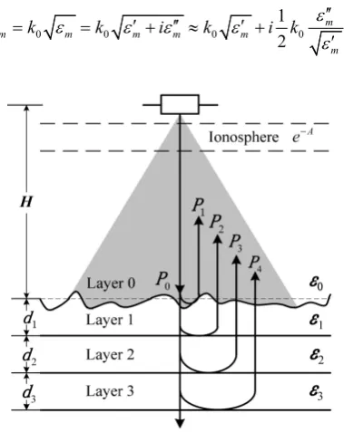
DOI: 10.4236/ijaa.2019.93024 337 International Journal of Astronomy and Astrophysics The SHARAD radar sounder data has shown that there are multi-layer struc-tures in Mars Polar regions [6]. When the sub-layer thickness varies little within one radar footprint, the multi-layer structure from the top to hundreds meters below can be modeled as a parallel-stratified media, as shown in Figure 1. As the electromagnetic (EM) wave of radar sounder is vertically incident upon the top surface through ionosphere, there would be multi-reflection and transmission through the media. Based on the difference of time delay of each echo from me-dia interfaces, and separating the rough surface clutter and the echoes of the in-terfaces, the echoes from each interface can be identified.

Suppose that multiple reflection and transmission between interfaces are neg-lected. It means that the echo from the n-th interface experienced one-reflection, round trip of 2(n − 1) transmissions (i.e. including round trip attenuation) through previous (n − 1) layer media. This assumption is based on small differ-ence on final surface reflectivity caused by underlying multi-layer structures. Thus, as the incident radar power through ionosphere is directly on the top sur-face P0=P0( )ae−A, the echo from the n-th interface is written as

(

)

1 2 0

1

exp 4

n

n n m m m

m

P P r − t k d

=

 ′′ 

=

∏

_ − _₍₁₎

where P0( )a is denoted as the transmitted power of dipole antenna (with

nota-tion (a)), and similarly, ( )a e A

n n

P ₌P − _{denotes the n-th reflected peak power} re-ceived by the radar antenna, i.e. observation. In Equation (1), tm is the trans-mittivity between the (m − 1)-th and the m-th media, rn is the reflectivity of the n-th layer, dm is the thickness of the m-th layer, km′′ is the imaginary part of the wave number of the m-th layer, exp 4

(

− k dm m′′

)

is the round-trip attenua-tion in the m-th layer [19], e−A_{is the one-way attenuation through ionosphere} layer. The wave number of the m-th layer is written as

0 0 0 1₂ 0 m

m m m m m

m

k k ε k ε iε k ε i k ε

ε ′′

′ ′′ ′

= = + ≈ +

[image:3.595.280.470.470.709.2]

′ (2)

(4)

DOI: 10.4236/ijaa.2019.93024 338 International Journal of Astronomy and Astrophysics Here k0 is the wave number of free space. ε ′m and ε ′′m are the real and im-aginary parts of the m-th layer dielectric constant, respectively. km′′ is written as

0

1

2 m

m

k k ε

ε ′′ ′′ =

′ (3)

The transmittivity satisfies

1

m m

t = −r ₍₄₎ and the layer thickness can be expressed as

2m m m c d τ ε

= ₍₅₎

where c is the light speed in free space, and τm is the time delay as EM wave propagates through the m-th medium twice, i.e. the time delay between two echoes from two successive interfaces.

Substituting Equations (3)-(5) into Equation (1), the reflected power from the n-th interface is derived as

(

)

(

)

(

)

1 ₂ 0 0 1 1 ₂ 0 0 1 1 exp

1 exp tan

n

m

n n m m

m m

n

n m m m

m

P P r r k c

P r r k c

ε

τ

ε

τ

δ

− = − =   ′′ =  − − _′         = _ − − _

∏

(6)

where tanδm=ε εm′′ ′m is the (attenuation) loss-tangent of the m-th layer. 2) Calculation of Loss Tangent

Since roughness of underlying interfaces is totally unknown, the model makes all underlying interfaces as plane-stratified, as shown in Figure 1. Equation (6) presents a set of total n equations, where Pn and τm can be found from the ra-dar data ( )a

n

P , but the incidence power directly upon the top surfaceP0, the

at-tenuation e−A_{, the reflectivities} 1, , n

r  r , and the loss tangents tan , , tanδ1 δn−1

are to be solved. Considering the ionosphere attenuation is wrapped into P0,

there are totally 2n independent unknowns in Equation (6).

It has been known from Mars studies that the loss tangents of NPLD and SPLD are actually very small, as usually 0.001 - 0.005 [1][3]. Some extreme cases of the media with high conductivity (dipolar and conductive) are excluded. In radar sounder technology for exploring multi-layering structure, whole media should be at a very low loss to make the wave penetration to reach the interfaces.

Certainly, the reflectivity r n_n

(

=1, , n−1

)

is a main factor to affect Pn, comparing with τm, tanδm and exp

(

−k c0

τ

mtan

δ

m

)

. To reduce the number of unknowns and reach final inversion, all small loss tangents of the n-layers are trivial and seen as the same within one illuminated area (e.g. 1.81 km in the next example). The low value of the loss tangent makes such approximation reasona-ble. Thus, Equation (6) is simplified as

(

)

1

1 ₂

0 0

1 1

exp tan n n 1

n n m m

m m

P P r k c

δ τ

− − r

= =

 

= _− _ −



∑



∏

(7)

(5)

DOI: 10.4236/ijaa.2019.93024 339 International Journal of Astronomy and Astrophysics

(

)

1 1

0 0

1 1

ln n tan n m ln ln n 2 ln 1n m

m m

P k c

δ τ

− P r − r

= =

= −

∑

+ + +

∑

− (8)

It means that the echo from each interface is a linear function of the time de-lay

(

0

)

,

lnPn= − k ctan

δ τ

total n+ +b

ξ

(9) where , 1

1 n

total n m

m

τ

−

τ

=

∑

is the time delay from the n-th interface echo to the top

surface echo, b is an unknown constant, ξ is a random variable to take account of different reflectivities, rn, of the interfaces.

Equation (9) can be seen as a linear regression model with the regress or

τ

_.

Using the radar range echoes from all interfaces and their respective ranges, the linear fitting is obtained with the least square method. Then the loss tangent can be calculated by the slope of linear function in Equation (9).

3) Solution of Dielectric Constant of Each Layer

Since the loss tangent is obtained, the number of unknowns now becomes n + 1. The set of Equation (7) can be directly solved, and the reflectivity is written as

(

)

1

1 ₂

0 0

1 1

exp tan 1

n

n _n _n

m m

P r

P k c δ τ− − r

= = = ₋  ₋   

∑



∏

(10)

Equation (10) can be solved, iteratively.

Reflectivity is a function of the dielectric constants of layering media. Because the roughness of all sub-interfaces is totally unknown, it is practicable to model all sub-interfaces between layers as flatly stratified within a limited area. This is a good and workable assumption within a limited area illuminated by the radar waves, even if a small error might be caused due to small scale roughness of the interfaces.

It is also noted that in derivation of Equation (1), multiple-reflection and transmission are neglected. Thus, the reflectivity from the (n − 1)-th layer to the n-th layer is derived based on a half-space model, i.e. the reflectivity of this in-terface is written as

2 1 1 n n n n n

r ε ε

ε ε − −  −  = _ _ +

  (11) Since the loss tangent is very small, it yields εm ≈ε ′m, Equation (11) becomes

2 1 2 ₁ 1 n n n r

ε ε −

 

′=_ − _ ′ ±

  (12) But, there would be two solutions from Equation (12) due to the term ± rn . Using the phase change of the echoes, an unique solution may be obtained.

The echo phase from the n-th interface is written as

1 1

0 0 , ,

1 1

2

n n

n m t m r n

m m

k c

ϕ

−

τ

−

ϕ

= =

(6)

DOI: 10.4236/ijaa.2019.93024 340 International Journal of Astronomy and Astrophysics where ϕ0 is the phase of EM incidence,

ϕ

t m, denotes the phase from each

transmission, and

ϕ

r n, the phase of each reflection.

As EM wave is vertically incident from the (n − 1)-th layer to the n-th layer, the reflection coefficient and transmission coefficient are, respectively, written as

1

n n

n

n n

R ε ε

ε ε

−

− =

+ (14)

1

2 _n

n

n n

T ε

ε ε −

=

+ (15)

Since the loss tangent is very small, it can be seen that if εn′ >εn′−1, it makes

0

n

R > _and

ϕ

_{r n}_, =0; otherwise, if εn′<εn′−1, it makes Rn<0 and

ϕ

r n, = π.

In transmission, the phase keeps unchanged, i.e.

ϕ

t m, =0.

As incident upon the top surface,

ϕ

r,1=0. Equation (13) gives ϕ0=ϕ1.

Thus, all phases due to reflections from all interfaces can be calculated from the data of radar range echoes as

1

, 1 0

1 n

r n n m

m k c

ϕ

ϕ ϕ

−

τ

=

= − −

∑

₍₁₆₎

Based on these approximations, it yields the dielectric constant of each layer as

2

1 ,

2

1 ,

2 ₁ ₀

1

2 ₁

1

n r n

n n

n r n

n r r ε ϕ ε ε ϕ − −   _ − _ ′ =  −   ′ =    ′

− = π

 

 ₊ 

 



(17)

4) Calculation of Ionospheric Attenuation and Dielectric Constant of the Sur-face Medium

Propagation through the ionosphere causes phase distortions and attenuation. The SHARAD Reduced Data Record (RDR) data has already corrected the phase distortion using Phase Gradient Autofocus (PGA) method [20]. The ionosphere is excited by solar radiation, and its effect during daytime is much stronger than during night [21][22] [23]. To avoid the additional error caused by phase dis-tortion, only data acquired during the night are specifically used in the following example. Moreover, ionospheric attenuation is taken into account using an uni-form constant e−A_{when the SHARAD data acquired with the similar solar} ze-nith angle (SZA).

Since the SHARAD data, as available, have not been absolutely calibrated [20], the simulated echo power from the interfaces used in the inversion [10] [24],

1, , n

P  P , should be adjusted to match the observations P1( )a, , Pn( )a on the radar receiver. It gives

( )a _e A _1,

₍

₎

n n n

P ₌P − _≡CP n₌ _ ₍₁₈₎

(7)

DOI: 10.4236/ijaa.2019.93024 341 International Journal of Astronomy and Astrophysics ionospheric attenuation.

It has been studied [25] that there is purely CO2 ice covering an area of the South Pole of Mars, and its dielectric constant is known as about 2.2. Thus, based on the observation data P1( )a

(

ε1=2 2.

)

, as available, and our simulated

data P1

(

ε

1=2 2.

)

at this South Pole location, C of Equation (18) is obtained

and applied to the whole inversion region.

The top surface is modeled as a rough surface, described by the known DEM data. From the radar equation [26], the echo from the top surface (with

ε

₎

un-der radar EM wave incidence (nadir incidence θ =i 0) is written as

( )

1 0

P

ε

=

γ ε

P₍₁₉₎ where γ is the backscattering coefficient of rough surface.

The Kirchhoff approximation (KA) of rough surface scattering requires the curvature radius of the surface much larger than the radar wavelength [19], it is a gentle rough surface on most areas on Mars. It has been discussed [11] that based on derivations of rough surface scattering with surface mean zero slope and the KA, the received echoes power at nadir direction is simply proportional to the surface reflectivity. It presented the inversion that the ratio of the received echo powers from one unknown and another tested surface permittivity can present inversions of the surface reflectivity, and dielectric unknown.

Thus, it is derived as [11]

( )

2 2 2 0 1

ei i d

k

r A

γ ε ε

′′

⋅ _′

=

π

∫∫

k r S

S

(20)

where ki is the incident wave vector, r′′ is the distance vector from the pixel center of integral to the nadir point.

Suppose that the top surface has a test value 0 1

ε

, the simulation gives

( )

0

1 1

P ε _. The ratio of the observation P1( )a

( )

ε1 with an unknown ε1 over the simulation

( )

0

1 1

CP ε _{with assumed} 0 1

ε

gives [10]

( )

_{( )}

( )

_{( )}

( )

1 1 1 1 0 1 1 1

0 0 0

0

1 1 0 1 1 1

1 1

.

a a

a

P P P C r

P C P C r

P

ε

γ ε

ε

γ ε

ε

= = = (21)

where C was defined in Equation (18), and actually can be evaluated in the next approach. Substituting Equation (11) into Equation (21), it gives the inverted

1

ε ′_{, as follows}

( )

_{( )}

( ) ( )

2

1

1 1 0

1 1

0

1 1

2 _{1 .}

1 Pa r

CP ε ε _ε ε         ′ = −    −      (22)

(8)

DOI: 10.4236/ijaa.2019.93024 342 International Journal of Astronomy and Astrophysics ignores those cases with steep slopes or highly varying roughness.

Using the inverted ε ′1 and Mars Orbiter Laser Altimeter (MOLA) elevation

data, the backscattering coefficient

γ ε

( )

1 can be calculated in our numerical

simulation [10][27]. It yields the incident power on the top surface, of Equation (10) as follows,

( )

1 1

0 1 P

P = _{γ ε}ε ₍₂₃₎

Substituting the inverted ε ′1,P0 and observation P2( )a into Equations (10), it

gives r2. Then, Equation (17) gives ε ′2. Sequentially, it yields

ε

n′

(

n=3,

)

, etc. The thickness of each layer can be then calculated by Equation (5).

3. Inversion of Dielectric Constants at the Promethei Lingula

of Mars South Polar Region

1) SHARAD Radar Echoes Data from the Promethei Lingula

[image:8.595.226.525.444.693.2]

As shown in Figure 2, the Promethei Lingula around Mars South Pole is a part of SPLD. Figure 3 presents one SHARAD observation over this region. The radargram in Figure 3 is composed of about 2500 echoes after pre-summing on board the spacecraft. The radar flight distance is about 90.5 km during 2500 times vertical sounding. A stratified structure can be well identified in SHARAD radargram. Figure 4 is the optical photo of High Resolution Image Science Ex-periment (HiRISE) around the cliff of Chasma Australe canyon on the west edge of the Promethei Lingula, which clearly shows the existence of stratifications of layering media [28].

(9)

[image:9.595.217.531.71.210.2]

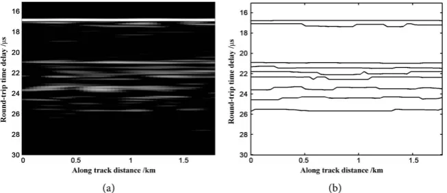
[image:9.595.268.477.257.339.2]

Figure 3. A portion of SHARAD track 17485_01 data from stratified media in Promethei Lingula.

Figure 4. The stratified structure on HiRISE photo of Chasma Australe canyon eastern cliff. (ESP_023590_0975_RED.abrowse.jpg on HiRISE website).

We choose the track 17485_01 of SHARADRDR data on PDS Geosciences node (filename: r_1748501_001_ss11_700_a.dat on website

http://pds-geosciences.wustl.edu/), which passes by Promethei Lingulanear the Chasma Australecanyon during the night (SZA is about 112˚), for inverting the parameters of multi-layer media. The vertical resolution of the data is 15m in vacuum and about 8.5 m in pure ice. The latitude and longitude of each frame are indicated in the SHARAD RDR data, and the along-track distance between each frame can be calculated. Especially, the distance between each frame in Figure 3 is about 36.2 m (0.00056˚ in latitude and 0.002˚ in longitude). Accord-ing to the radargram and optical image, the topography and interfaces below the top surface look almost flat for one radar footprint. It validates our flatly strati-fied media model for Promethei Lingula.

2) Echoes from the Surface/Sub-Surfaces and Interface Locations

(10)

DOI: 10.4236/ijaa.2019.93024 344 International Journal of Astronomy and Astrophysics flat interfaces has little change as radar is moving, and usually shows straight line in radargram. Based on this intuition, we define a threshold S to decide if the echo is from the subsurface or not:

( )

, 1

(

,

)

2

m n

q m p n

S i j s i q j p

n =− =−

=

∑ ∑

+ + ₍₂₄₎

where

( )

, 1 the -th sample of frame is local maximum 0 the -th sample of frame is not local maximum

i j

S i j

i j

 = 

 .

For example, let n = 25 and m = 1, and hence S indicates the ratio of local maximum from totally nearby 50 frames with the similar time delay (not ex-ceeding 1 sampling interval). If S>0.7_{, it means that more than 70% of}

adja-cent frames have reflector with the same time delay, and the reflector is judged to be from the interface. Otherwise, the isolated reflector is seen as the surface clutter. In this way, the surface echoes and interface echoes are distinguished from frame 69,301 - 69,350 of the track 17485_01, which extends about 1.81 km.

Finally, the stratification of multi-interfaces is shown in Figure 5. Not all the reflectors in Figure 5(a) are kept in Figure 5(b). Some short lines and bright points are erased, and only are kept those long lines. If a few adjacent pixels on the long line happen to be weak and break the continuity of the extracted inter-face, the weak pixels are artificially fixed and judged as interface to avoid layer-ing discontinuity. Linear interpolation of the interface line is used to decide the interface ranges of weak pixels. And the power of the nearest pixel is judged as the echo power of the interface.

Thus, the surface echoes, the echoes from underlying interfaces, i.e. P nn, =2,,

[image:10.595.211.538.553.694.2]

can be obtained. Sometimes, the echoes from different locations of the same interface might be quite different. It might be caused by different interface- topography, or happens to be mixed by the surface clutters. Dimmer or brighter radar echoes may also be caused by the change of interface reflectivity or the change of the interface time delay, for the time delay changes lead to different interference in the radar signal. To avoid such fluctuations of the interface echoes to affect final inversion, the echoes from the same interface is taken as an averaged value.

(11)

DOI: 10.4236/ijaa.2019.93024 345 International Journal of Astronomy and Astrophysics 3) Dielectric Constant of the Surface Medium

Figure 6(a) shows the surface radar echoes power acquired from SHARAD in South Polar Region, where the central white circle is no-data region. The surface echo (the strongest peaks in each frame) from each area is taken from SHARAD data are used to generate Figure 6(a), which covers most part of SPLD. Similar figures had been done by Grima et al. [30] (Mars surface reflectivity map of SHARAD) and Mouginot et al. [12] (Mars surface reflectivity map of MARSIS).

Using the MOLA (Mars Orbiter Laser Altimeter) elevation data, the surface echoes from this rough surface can be numerically simulated [10][27]. At the beginning, we take a proposed dielectric constant 0

1 3

ε

= _{over whole area,} which is similar to the water ice. And 0

1 3

ε

= _{is used for the echoes simulation} around Mars South Polar region. The simulated

( )

0

1 1

P′ ε _{is obtained as shown} in Figure 6(b).

The ratio of Figure 6(a) over Figure 6(b), i.e. 1_{( )}( )

_{( )}

( )

1 0

1 1

a

a P P

ε

of Equation (21), is

[image:11.595.219.530.391.681.2]

shown in Figure 6(c). It has been studied [25] that there is thick purely CO2 ice cap covering the South Pole, which can be also seen from blue colors of Figure 6(a) and Figure 6(c). The dielectric constant of CO2 is much lower than water ice and rocks. So the echo power of CO2 cap is much less than other places. The constant of C, Equation (18), is actually obtained from these figures.

(12)

DOI: 10.4236/ijaa.2019.93024 346 International Journal of Astronomy and Astrophysics Using the algorithm aforementioned, the dielectric constant of Mars surface over the South polar region, ε ′1, can be inverted, as shown in Figure 6(d). The

inverted results are influenced by the seasonal CO2 ice, because the data used in the inversion are all acquired during autumn and winter, and the Mars polar re-gions are covered by a thin CO2 ice layer less than 1 m thick at that time [31]. Some studies show that the radar echo power decreases when a thin CO2 ice covers on the top player [24]. Since the covering of seasonal CO2 ice is variable and uncertain for data acquired in different time, which is much thinner in terms of SHARAD resolution, the inverted dielectric property of the first layer can be seen as the effective dielectric constant including thin CO2 ice layer as available. The inverted results are the equivalent dielectric constants of a cluster of thin layers comprised of CO2 ice and water ice with dust. The ε ′1 of most

areas of SPLD is between 3 and 4. These results show that SPLD is mainly com-prised of water ice, which is consistent with previous studies [7][32]. However, there are still some areas of SPLD in Figure 6(d) having ε ′1 larger than 4,

in-cluding the Promethei Lingula. It can be seen that the areas with large ε ′1 are

all located in the outer part of SPLD, which does mean that these areas may contain more impurity than the center of SPLD. Certainly, low resolution of MOLA data (except the data near the pole, which has a high resolution) as available, to describe complex rough surface might cause inversion error. The typical Root Mean Square heights over the SPLD at SHARAD scales is ~0.30 m [30], which is smaller than the MOLA resolution of 1 m, which might cause an error in inversion.

4) Calculation of Loss Tangent

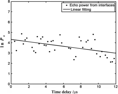
To reduce the fluctuation of different reflectivities of the interfaces (ξ in Equation (9)), the echoes powers of the interfaces with the same time delay are averaged. Using the least square method to make a linear fitting for the average echoes power with different time delay, a linear equation of

5 ,

lnPn= −1.11 10× τtotal n+4.3 is obtained, as shown in Figure 7. From Equation

(9), it yields 5

( )

0

tanδ =1.11 10× k c =0.00088_{. The confidence interval of loss}

[image:12.595.271.474.543.705.2]

tangent with the confidence level of 95% is [0.0004, 0.0014].

(13)

[image:13.595.256.491.75.262.2]

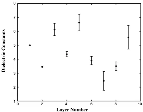
[image:13.595.254.492.298.487.2]

Figure 8. Dielectric constant of each layer (along track).

Figure 9. Dielectric constant of each layer (across track).

[image:13.595.254.491.522.707.2]

(14)

DOI: 10.4236/ijaa.2019.93024 348 International Journal of Astronomy and Astrophysics The hypothesis of linear regression model to well fit the data is tested using F distribution. It takes F =13.1_{for total 42 data points in the linear fitting.}

Set-ting the significant level α =0.01_{, it gives} Fα

(

1,40

)

=7.31 and F F> α

(

1,40

)

. Thus, the linear regression is good to fit the data. The loss tangent is much smaller than previous result [1][3], which contained both absorption of martials and signal loss at each interface reflection [1], while in our inversion, the signal losses of the interface reflections are totally removed, as shown in Equation (8).

5) Echoes Phase Estimation and Unique Solution Determination

The sampling interval of the SHARAD data is 0.075 μs [20], which corres-ponds to the depth of 0.75 wavelength in free space according to Equation (5). It would be difficult to obtain enough accurate phase information as the radar wave propagates through the layers. Firstly, we interpolate each frame data using sinc function [33]. Then, the local maximum of the interpolated data is judged as the new interface instead of the interface extracted before. Thus, the time delay of each interface can be estimated accurately. Then, the phases are calculated by Equation (16). Due to surface clutter interference, there are noises in the phases which make errors during the phase evaluation. We take an average of the phas-es of echophas-es from the same interface to reduce the errors.

(

)

69350

, 69301

Im ln exp

n n f

f i ϕ ϕ =      =      



∑

 (25)

where

ϕ

n f, is the phase of frame f and n-th interface.

Substituting Equation (25) into Equation (16), the phase of reflection is calcu-lated. Considering that

ϕ

r n, usually is not exactly equal to 0 or π due to the

phase accuracy, Equation (17) is changed as

2

1 ,

2

1 ,

2 ₁ _,

2 2 1

2 ₁ _, _,

2 2

1

n r n

n n

n r n

n r r ε ϕ ε ε ϕ − −

  _ _{π π}_

_ ₋ _ _′ _{∈ −}_ _

 

 −  

 

′ = 

  _ _π_{ }_π _

′

− = −π − π

  _ _ _ _{ } _ +         (26)

6) Inversions and Validation

The dielectric constant of surface medium ε ′1 inverted from the frame

69,301 - 69,350 (83˚S 102˚E in Figure 6(d)) of the track17485_01 is about 5 (see the location of Layer 1 at elevation 2100-2200 in Figure 8 and Figure 9. Note that the layer 0 on the top of Figure 8 and Figure 9 is Mars atmosphere). This result may be overestimated as discussed in part C of section II. However, it is possible that Layer 1 of Promethei Lingulacontain more impurity than the center of SPLD. Thus we choose ε ′ =1 5.

Substituting ε ′1 into Equation (25), and changing the loss tangent from

(15)

DOI: 10.4236/ijaa.2019.93024 349 International Journal of Astronomy and Astrophysics be seen as pure ice.

Using Equation (5), the thickness of each layer is calculated, as shown in Fig-ure 8. There won’t be echo from the place below Layer 9, since EM wave there-has become very weak due to transmission and reflection. Thus, the dielectric constant below 1500 m in Figure 8 is actually unknown, and the thickness of layer 9 cannot be inverted.

The inversion accuracy depends on the evaluation of interface locations and echo powers. The phase accuracy might be also interfered by surface clutter.

Suppose the depth of each interface do not change across the track, as shown in Figure 9. The red point in Figure 9 is the nadir of track 17485_01 and the dashed line is the stratification in Figure 8. Then the position of each interface exposed on the cliff can be calculated using MOLA elevation. To validate our inversions, the calculated interface exposed on the cliff is projected to a map-projected optical image, as shown in Figure 11. Note that Figure 8 gives the vertically layering structure, while Figure 11 shows a slant section of the cliff photographed vertically downwards

[image:15.595.247.500.542.694.2]

It can be seen that the inverted multi-layering structure is well described on the cliff of Chasma Australe canyon near track 17485_01, which was indicated in a HiRISE optical image, even not exactly the same matching. The optical layers are much finer than the radar resolution, and they cannot be a 1:1 correlation. The layers in radargram correspond to the packets of thinner layers in optical image. Many layers can be seen on optical image but cannot be detected by ra-dar, because this HF radar technology is capable only to detect the interfaces with a significant change of dielectric media. The inversion model presented is based on the implicit assumption that there is no more than one such interface within a SHARAD vertical resolution (10 - 15 m). If SHARAD reflections are caused by merged reflections of packets of thinner layers with different dielectric constants, the inversed layer-depths and dielectric properties are understood on the average or effective sense for radar sounder echoes. Moreover, details of the technology parameters and measurements, such as SNR for each echo and high resolution elevation data might further improve the inversions.

(16)

DOI: 10.4236/ijaa.2019.93024 350 International Journal of Astronomy and Astrophysics The inversion results show that the dielectric deposits in Promethei Lingula are not uniformly stratified, seen along the dashed line indicated in Figure 9. Most layers seem nearly pure ice (e.g. blue colors), but some thin layers includ-ing the surface layer are with a lot of dust (e.g. yellow colors). As the deposit is seen as a component of ice and dust, its dielectric constant is written as [34]

(

)

1 1

3 3 3

dust ice dust dust

1 c c

ε=_ − ε + ε _

  (27) where cdust is the dust fraction, and can be calculated as

1 1

3 3

1 1

3 3

ice dust

dust ice

c

ε

− =

− (28)

Taking the dust basalt (εdust =8), the dust fraction is calculated using

Equa-tion (28), as shown in Figure 11. Layer 3 and Layer 5 have a dust load of 60% - 70%, which means these layers may be a compact frozen ground (permafrost) rather than dirty ice. However, SHARAD reflections might be caused by thinner layers, on the order of a meter thick or so [35][36]. Packets of low dust thin lay-ers with a few thin permafrost laylay-ers might be another possible existence of Lay-ers 3 and 5. Thus, it is possible to overestimate the dust fraction in the invLay-ersion.

Making a dielectric average of top 8 layers media, it yields

8 8

1 i i 1 i

i d i d

ε

= =

=

∑

(29)

It gives the dielectric constant of regolith impurity,

ε

=3.6_{, which}

corres-ponds to the dust fraction about 12%.

4. Conclusions

This paper presents a model of rough surface and stratified interfaces to describe the multi-layer structure of Mars Polar Layered Deposit. The range echoes of HF radar sounder from rough surface/subsurface is numerically calculated. And under the Kirchhoff approximation with a mean zero slope, the received echo at nadir direction preserves the functional dependence of the surface reflectivity. In radargram to show the radar range echoes, the nadir surface echo and the echoes from layering interfaces are separated from off-nadir surface clutters. As the surface dielectric constant is derived from the ratio of the received echo peak power, the inversion approach is designed to obtain the dielectric constant and layer thickness of next layers, sequentially.

(17)

DOI: 10.4236/ijaa.2019.93024 351 International Journal of Astronomy and Astrophysics be taken into account, the inversion accuracy can be further improved.

The inversion model is based on the assumption that there is no more than one interface within a SHARAD vertical resolution. As SHARAD reflections might be caused by packets of thinner layers, multi-layer model under this reso-lution won’t be able to see them, individually, which are merged with other stronger adjacent reflections. The inversed layer-depths and dielectric properties are understood on the average or effective sense for radar sounder echoes.

Acknowledgements

This work was supported by the National Key Research and Development Pro-gram of China 2017YFB0502703.

The MOLA elevation data and SHARAD Reduced Data Record (RDR) data are all from PDS Geosciences Node (website:http://pds-geosciences.wustl.edu/). The HiRISE optical data are from the HiRISE website (http://hirise.lpl.arizona.edu/).

Conflicts of Interest

The authors declare no conflicts of interest regarding the publication of this pa-per.

References

[1] Grima, C., Wlodek, K., Jérémie, M., Phillips, R.J., Alain, H., Daniela, B., Roberto, S. and Marco, C. (2009) North Polar Deposits of Mars: Extreme Purity of the Water Ice. Geophysical Research Letters, 36, 151-157.

https://doi.org/10.1029/2008GL036326

[2] Phillips, R.J., Zuber, M.T., Smrekar, S.E., Mellon, M.T., Head, J.W., Tanaka, K.L., Putzig, N.E., Milkovich, S.M., Campbell, B.A. and Plaut, J.J. (2008) Mars North Po-lar Deposits: Stratigraphy, Age, and Geodynamical Response. Science, 320, 1182-1185. https://doi.org/10.1126/science.1157546

[3] Plaut, J.J., Giovanni, P., Ali, S., Ivanov, A.B., Milkovich, S.M., Andrea, C., Wlodek, K., Jérémie, M., Farrell, W.M. and Phillips, R.J. (2007) Subsurface Radar Sounding of the South Polar Layered Deposits of Mars. Science, 316, 92-95.

https://doi.org/10.1126/science.1139672

[4] Fishbaugh, K.E., Byrne, S., Herkenhoff, K.E., Kirk, R.L., Fortezzo, C., Russell, P.S. and Mcewen, A. (2010) Evaluating the Meaning of “Layer” in the Martian North Polar Layered Deposits and the Impact on the Climate Connection. Icarus, 205, 269-282. https://doi.org/10.1016/j.icarus.2009.04.011

[5] Hvidberg, C.S., Fishbaugh, K.E., Winstrup, M., Svensson, A., Byrne, S. and Her-kenhoff, K.E. (2012) Reading the Climate Record of the Martian Polar Layered De-posits. Icarus, 221, 405-419. https://doi.org/10.1016/j.icarus.2012.08.009

[6] Seu, R., Phillips, R.J., Giovanni, A., Daniela, B., Francesco, B., Marco, B., Diego, C., Campbell, B.A., Marco, C. and Carter, L.M. (2007) Accumulation and Erosion of Mars’ South Polar Layered Deposits. Science, 317, 1715-1718.

(18)

[8] Seu, R., Biccari, D., Orosei, R., Lorenzoni, L.V., Phillips, R.J., Marinangeli, L., Picar-di, G., Masdea, A. and Zampolini, E. (2004) SHARAD: The MRO 2005 Shallow Ra-dar. Planetary & Space Science, 52, 157-166.

https://doi.org/10.1016/j.pss.2003.08.024

[9] Seu, R., Phillips, R.J., Daniela, B., Roberto, O., Arturo, M., Giovanni, P., Ali, S., Campbell, B.A., Plaut, J.J. and Lucia, M. (2007b) SHARAD Sounding Radar on the Mars Reconnaissance Orbiter. Journal of Geophysical Research Planets, 112, 37-55. https://doi.org/10.1029/2006JE002745

[10] Liu, C., Ye, H. and Jin, Y.Q. (2014) Simulation of Radar Echoes from Mars’ Sur-face/Subsurface and Inversion of Surface Media Parameters. Radio Science, 49, 473-484. https://doi.org/10.1002/2013RS005367

[11] Ye, H. and Jin, Y.Q. (2013) An Inversion of Planetary Rough Surface Permittivity From Radar Sounder Observations. IEEE Antennas & Wireless Propagation Letters, 12, 1069-1072. https://doi.org/10.1109/LAWP.2014.2329425

[12] Mouginot, J., Pommerol, A., Kofman, W., Beck, P., Schmitt, B., Herique, A., Grima, C., Safaeinili, A. and Plaut, J.J. (2010) The 3-5 MHz Global Reflectivity Map of Mars by MARSIS/Mars Express: Implications for the Current Inventory of Subsurface H2O. Icarus, 210, 612-625. https://doi.org/10.1016/j.icarus.2010.07.003

[13] Nouvel, J.F., Martelat, J.E., Herique, A. and Kofman, W. (2006) Top Layers Chara-terization of the Martian Surface: Permittivity Estimation Based on Geomorphology Analysis. Planetary & Space Science, 54, 337-344.

https://doi.org/10.1016/j.pss.2005.12.013

[14] Lauro, S.E., Mattei, E., Soldovieri, F. and Pettinelli, E. (2012) Dielectric Constant Estimation of the Uppermost Basal Unit Layer in the Martian Boreales Scopuli Re-gion. Icarus, 219, 458-467. https://doi.org/10.1029/2010GL043015

[15] Mouginot, J., Antoine, P., Pierre, B., Wlodek, K. and Clifford, S.M. (2012) Dielectric Map of the Martian Northern Hemisphere and the Nature of Plain Filling Materials.

Geophysical Research Letters, 39, L02202-L02206. https://doi.org/10.1029/2011GL050286

[16] Zhang, Z. and Nielsen, E. (2011) Using Complex Independent Component Analysis to Extract Weak Returns in MARSIS Radar Data and Their Possible Relation to a Subsurface Reflector on Mars. Radio Science, 46, 599-609.

https://doi.org/10.1029/2010RS004426

[17] Zhang, Z., Hagfors, T., Nielsen, E., Picardi, G., Mesdea, A. and Plaut, J.J. (2008) Di-electric Properties of the Martian South Polar Layered Deposits: MARSIS Data In-version Using Bayesian Inference and Genetic Algorithm. Journal of Geophysical Research, 113, E05004. https://doi.org/10.1029/2007JE002941

[18] Alberti, G., Castaldo, L., Orosei, R., Frigeri, A. and Cirillo, G. (2012) Permittivity Estimation over Mars by Using SHARAD Data: The Cerberus Palus Area. Journal of Geophysical Research, Atmospheres, 117, 371-387.

https://doi.org/10.1029/2012JE004047

[19] Jin, Y.Q. (1994) Electromagnetic Scattering Modelling for Quantitative Remote Sensing. World Scientific, Singapore. https://doi.org/10.1142/2253

[20] Slavney, S. and Orosei, R. (2007) Shallow Radar Reduced Data Record Software In-terface Specification.

[21] Safaeinili, A., Kofman, W., Nouvel, J.-F., Herique, A. and Jordan, R.L. (2003) Im-pact of Mars Ionosphere on Orbital Radar Sounder Operation and Data Processing.

(19)

[22] Mouginot, J., Kofman, W., Safaeinili, A. and Herique, A. (2008) Correction of the Ionospheric Distortion on the MARSIS Surface Sounding Echoes. Planetary and Space Science, 56, 917-926. https://doi.org/10.1016/j.pss.2008.01.010

[23] Campbell, B.A., Putzig, N.E., Foss, F.J. and Phillips, R.J. (2014) SHARAD Signal At-tenuation and Delay Offsets Due to the Martian Ionosphere. IEEE Geoscience and Remote Sensing Letters, 11, 632-635. https://doi.org/10.1109/LGRS.2013.2273396

[24] Mouginot, J., Kofman, W., Safaeinili, A., Grima, C., Herique, A. and Plaut, J.J. (2009) MARSIS Surface Reflectivity of the South Residual Cap of Mars. Icarus, 201, 454-459. https://doi.org/10.1016/j.icarus.2009.01.009

[25] Phillips, R.J., Davis, B.J., Tanaka, K.L., Shane, B., Mellon, M.T., Putzig, N.E., Ha-berle, R.M., Kahre, M.A., Campbell, B.A. and Carter, L.M. (2011) Massive CO2 Ice

Deposits Sequestered in the South Polar Layered Deposits of Mars. Science, 332, 838-841. https://doi.org/10.1126/science.1203091

[26] Ulaby, F.T., Moore, R.K. and Fung, A.K. (1981) Microwave Remote Sensing Active and Passive. Artech House, New York.

[27] Fa, W.Z. and Jin, Y.Q. (2010) Simulation of Radar Sounder Echo from Lunar Sur-face and SubsurSur-face Structure. Science China Earth Science, 53, 1043-1055. https://doi.org/10.1007/s11430-010-3070-8

[28] Milkovich, S.M., Plaut, J.J., Safaeinili, A., Picardi, G., Seu, R. and Phillips, R.J. (2009) Stratigraphy of Promethei Lingula, South Polar Layered Deposits, Mars, in Radar and Imaging Data Sets. Journal of Geophysical Research, Atmospheres, 114, 1779-1794. https://doi.org/10.1029/2008JE003162

[29] Christian, S., Holt, J.W., Byrne, S. and Fishbaugh, K.E. (2013) Integrating Radar Stratigraphy with High Resolution Visible Stratigraphy of the North Polar Layered Deposits, Mars. Icarus, 226, 1241-1251. https://doi.org/10.1016/j.icarus.2013.07.003

[30] Grima, C., Kofman, W., Herique, A., Orosei, R. and Seu, R. (2012) Quantitative Analysis of Mars Surface Radar Reflectivity at 20 MHz. Icarus, 220, 84.

https://doi.org/10.1016/j.icarus.2012.04.017

[31] Piqueux, S., Kleinbohl, A., Hayne, P.O., Kass, D.M., Schofield, J.T. and McCleese, D.J. (2015) Variability of the Martian Seasonal CO2 Cap Extent over Eight Mars

Years. Icarus, 251, 164-180. https://doi.org/10.1016/j.icarus.2014.10.045

[32] Zuber, M.T., Phillips, R.J., Andrews-Hanna, J.C., Asmar, S.W., Konopliv, A.S., Le-moine, F.G., Plaut, J.J., Smith, D.E. and Smrekar, S.E. (2007) Density of Mars’ South Polar Layered Deposits. Science, 317, 1718-1719.

[33] Cumming, I.G. and Wong, W.C. (2005) Digital Processing of Synthetic Aperture Radar Data: Algorithm and Implementation. Artech House, Boston.

[34] Looyenga, H. (1965) Dielectric Constants of Heterogeneous Mixtures. Physica, 31, 401-406. https://doi.org/10.1016/0031-8914(65)90045-5

[35] Fishbaugh, K.E., Hvidberg, C.S., Shane, B., Russell, P.S., Herkenhoff, K.E., Mai, W. and Rolph, K. (2010b) First High-Resolution Stratigraphic Column of the Martian North Polar Layered Deposits. Geophysical Research Letters, 37, 256-265.

https://doi.org/10.1029/2009GL041642

[36] Nunes, D.C. and Phillips, R.J. (2006) Radar Subsurface Mapping of the Polar Layered Deposits on Mars. Journal of Geophysical Research, Planets, 111, 107-109.