An Evolutionary Algorithm Coupled to an Outranking Method for the Multicriteria Shortest Paths Problem

(1)

ISSN Online: 2160-8849 ISSN Print: 2160-8830

DOI: 10.4236/ajor.2019.93007 May 31, 2019 114 American Journal of Operations Research

An Evolutionary Algorithm Coupled to an

Outranking Method for the Multicriteria

Shortest Paths Problem

Frédéric Guidana Gazawa

1*

, Kolyang

2

, Irépran Damakoa

3

1_{Department of Mathematics and Computer Science, Faculty of Science, The University of Ngaoundere, Ngaoundere, Cameroon} 2_{Department of Computer Science, Higher Teacher’s Training College, The University of Maroua, Maroua, Cameroon}

3_{Department of Applied Mathematics and Computer Science, School of Geology and Mining Engineering, The University of} Ngaoundere, Ngaoundere, Cameroon

Abstract

In this article, we are interested in solving a combinatorial optimization problem, the shortest path problem in a multi-attribute graph, by the out-ranking methods. A multi-attribute graph has simultaneously qualitative and quantitative criteria. This situation gives rise to incomparable paths thus forming the Pareto front. Outranking methods in Multi-criteria Decision Making (MCDM) are the only methods that can take into account this situa-tion (incomparability of acsitua-tions). After presenting the categories of Mul-ti-criteria Decision Making (MCDM) and the difficulties related to the prob-lems of the shortest paths, we propose an evolutionary algorithm based on the outranking methods to solve the problem of finding “best” paths in a mul-ti-attribute graph with non-additive criteria. Our approach is based on the exploration of induced subgraphs of the outranking graph. Properties have been established to serve as algorithmic basis. Numerical experiments have been carried out and the results presented in this article.

Keywords

Multi-Criteria Decision Making, Evolutionary Algorithm, Shortest Path, Outranking Method, Induced Subgraphs

1. Introduction

The concept of relations was born out of difficulties encountered with diverse concrete outranking problems [1]. They can handle simultaneously qualitative and quantitative criteria. Criteria scores can be left in their own units, which is

How to cite this paper: Gazawa, F.G., Kolyang and Damakoa, I. (2019) An Evolu-tionary Algorithm Coupled to an Out-ranking Method for the Multicriteria Shortest Paths Problem. American Journal of Operations Research, 9, 114-128.

https://doi.org/10.4236/ajor.2019.93007

Received: January 30, 2019 Accepted: May 28, 2019 Published: May 31, 2019

http://creativecommons.org/licenses/by/4.0/

(2)

DOI:10.4236/ajor.2019.93007 115 American Journal of Operations Research important when they are related to diverse domains (e.g. economics, ecology and sociology). This method makes it possible to take into account the incompara-bility of actions. Outranking methods are the only methods that can take into account this situation [2] [3]. Unfortunately, outranking methods are not able to compare a lot of alternatives ([3] [4] [5]). For that, [6] [7] [8] argue that the out-ranking methods seem inappropriate for land suitability assessment.

Although this method is simple and allows a very thorough analysis of the robustness, this limitation makes several researchers prefer to use the MAUT (multiple attribute utility theory) method. This other approach tries to define a complete pre-order on the set of alternatives. Most often, the formal rules con-sist in mathematical formulas that lead to an explicit definition of a unique crite-rion synthesizing the m criteria. The weaknesses that result from this method are the reduction of the multicriteria problem into a unique criterion problem. The consequence of this reduction is that all the actions are comparable, a property that is not always desirable to have because one observes that for a human deci-sion-maker, there are situations involving incomparable alternatives [9]. More-over, it is often difficult to gather all the criteria of the decision-maker in a single criterion, and sometimes impossible to model such a function in a relevant way.

In view of the above, we thought it would be useful to find a way to overcome the weakness of limiting alternatives using the outranking method. In our work, we want to show that it is possible to remove this limitation. Instead of searching for the “best” solutions directly in the outranking graph, which is impossible if there are a very large number of alternatives, we show how to iteratively explore its induced subgraphs. To test our approach, we applied it to the shortest paths problem in a multi-attribute graph.

In the first part, we present the basic concepts related to Multi-criteria Deci-sion Making, multi-attribute graphs, difficulties in finding the shortest multicri-teria path and the SPARTE (Solution au PARadoxe de voTE—Solution to the voting paradox) outranking method which is very close to the ELECTRE (ELi-mination Et Choix Traduisant la REalité—eli(ELi-mination and choice expressing re-ality) outranking method. In the second part, we introduce our method by de-scribing some properties that we will use as algorithmic basis. Finally, we present in the third part our numerical experiments and the results obtained.

2. Background Concepts

2.1. Notations

( ) ( )

(

,

)

G= V G E G _{: graph}_G_{defined by the set of vertex}_V(G)_{and the set of}

edge E(G);

Gc: condensed graph of the graph G;

P(s, t): set of all elementary (s, t)-paths; Kr[G] or Kr:Reduced Kernel of a graph G; K[G] or K: Kernel set of a graph G;

( )

p

(3)

DOI: 10.4236/ajor.2019.93007 116 American Journal of Operations Research

k

δ _{: weight of criterion}_k;

wk(u, v): Evaluation of edge (u, v) according to criterion k;

Wk(p): Evaluation of the path p on the criterion k;

( )

(

1

( )

, 2

( )

, , m

( )

)

W p = W p W p _W p _{: Evaluation of the path}_p_on_m_criteria.

2.2. Multi-Attribute Decision Making

Multi-criteria Decision Making (MCDM) is classified into two general catego-ries: multi-objective decision making (MODM) and multi-attribute decision making (MADM) [10] [11], based on the different purposes and different data types. In the MADM problems, the decision-maker must choose from among a finite number of explicitly identified alternatives, characterized by multiple attributes, where these attributes define the decision criteria. The methods for dealing with MADM problems can be mainly divided into multiple attribute utility theory (MAUT) and outranking methods (especially refer to ELECTRE [12] [13] and PROMETHEE (Preference Ranking Organisation METHod for Enrichment Evaluations) methods [14]).

2.3. Graph

1) Definitions and notation

A graph G is a pair of sets (V, E), where V is the set of vertices and E is the set of edges, formed by pairs of vertices. In order to avoid any possible confusion, the vertex set of a graph G is denoted by V(G) and its edge set by E(G). A di-rected graph (or just digraph) G consists of the directed edges. A digraph H is a subdigraph of a digraph G if V H

( )

⊆V G

( )

_, E H

( )

⊆E G

( )

_{and every edge}

in E(H) has both end-vertices in V(H). If every edge of E(G) with both end-vertices in V(H) is in E(H), we say that H is induced by V(H) and H is called an induced subdigraph of G. A strongly connected component H of the digraph G is a directed subgraph of G (not a null graph) such that H is strongly connected, but if we add any vertex or edge to it, then it is not strongly connected anymore. The condensed graph Gc of the digraph G is obtained by contracting all the

edges in every strongly connected component. A subset K G

[ ]

⊆V G

( )

_{is a}

kernel if it is independent and absorbing/dominating. K[G] is dominating if

[ ]

, / ,

( )

u K G v v u E G

∀ ∈ ∃ ∈ . It is independent if ∀u v K G v u, ∈

[ ]

, ,

( )

∉E G

( )

. A kernel represents a set of winning positions in a graph [15].

2) Multi-Attribute graph

Let G = (V, E) be a directed and connected graph. Without loss of generality, we only considered the graph in which there exists at most one edge between a pair of ordered nodes. For a given graph, each edge connecting two nodes u and v is specified by a weight vector ω

( )

u v, =

(

ω1

( )

u v, ,ω2

( )

u v, , , ωm

( )

u v,

)

where ω_k

( )

u v k, , =1,2, ,_ m_{is the evaluation of the edge}e=

( )

u v, ∈E

ac-cording to the criterion (or point of view) k. m representthe number of criteria. Each criterion is associated with a value δk representing its weight.

(4)

DOI:10.4236/ajor.2019.93007 117 American Journal of Operations Research

( )

,

k u v

ω can be expressed in words (for example, “very bad”, ..., “average”, ..., “very good”) or letters with which numbers are associated to insist on the order that exists between these words/letters. In this case, they are ordinal numbers. They do not have an algebraic structure, which prohibits the use of arithmetic operations (for example addition “+”, multiplication “×”) on such numbers.

2.4. Shortest Paths Problem in Multi-Attribute Graph

Given a directed graph G = (V, E), an origin s V∈ and a destination t V∈ ,

the shortest-path problem (SPP) aims to find the minimum distance path in G

from s to t. The Multi-Attribute Shortest Paths Problem is an extension of the traditional shortest path problem and is concerned with finding a set of efficient paths with respect to two or more criteria that are usually in conflict and in-commensurable. In MODM, the problem is known to be NP-hard [16] [17]. The objectives are usually conflicting and there exists no best solution to the prob-lem, but a set of Pareto optimal solutions representing the best compromise among the objectives [18] [19].

Let P s t

( )

, denote the set of all s-t paths in G. If a path p=

(

e e1, , ,2  eL

)

( )

,

P s t

∈ _{. Its evaluation is the vector}W p

( )

=

(

W p W p₁

( )

, ₂

( )

, ,W pm

( )

)

where W pk

( )

is the path evaluation according to the criterion k. If k is a

quan-titative criterion, k

( )

k

( )

e p

W p ω e

∈

=

∑

_, k=1,2, ,_ m_{(additive criterion). When} k is a qualitative criterion, W pk

( )

=opt

(

ωk

( )

e1 ,ωk

( )

e2 , , ωk

( )

eL

)

(Non-additive

criterion) where “opt” may be one of the following operator min, max, median, mean, etc.

In general a multi-criteria shortest path is a kind of vector optimization prob-lem, which can be described as follows:

( ),

( )

(

1

( )

2

( )

)

Minimize_{p P s t}_∈ W p = W p W p, , ,W pm

“ ” . To solve this problem, we have

two large groups of approach.

The first one is called traditional approach. It can be characterized by assign-ing a well-defined degree to the m performances

(

W p W p1

( )

, 2

( )

, ,W pm

( )

)

values. Most often a numerical value v p

( )

= Ψ

(

W p W p1

( )

, 2

( )

, ,W pm

( )

)

is

assigned to each p P s t∈

( )

, _{on an appropriate scale. The way the aggregation} problem is addressed in this approach leads to define a complete pre-order on the set P s t

( )

, . Most often, the formal rules consist in mathematical formulas that lead to an explicit definition of a unique criterion synthesizing the m crite-ria. This is the case with MAVT, MAUT, SMART, TOPSIS, MACBETH, AHP, etc. The complete preorder on the set P s t

( )

, can be established. We usually find a better solution than all the others. In anyway, this approach does not allow any incomparability [20]. However, in a real traffic situation, the decision maker is not content with one solution but with a set of more effective solutions to make his own choice.

(5)

outranking methods (mainly PROMETHEE and ELECTRE methods). For the

choice problematic (P.

α

) solving the problem consists of two parts: construc-tion of an outranking graph, and exploitaconstruc-tion of the graph corresponding to this relation. The subset searched is the kernel of the graph [20].

2.5. Outranking Method SPARTE

The SPARTE outranking method [21] is based on the general approach of the ELECTRE outranking methods. Let p and q be two paths belonging to the set

( )

,

P s t . It is possible to build the following sets of indices:

• _{J p q}+

(

,

)

₌

{

_{j W p}/ j

( )

_>_{W q}j

( )

}

_{, the set of criteria for which the path}_p_is

preferred to the path q.

• _{J p q}−

(

,

)

₌

{

_{j W p}/ j

( )

_<_{W q}j

( )

}

_{, the set of criteria for which the path}_q_is

preferred to the path p.

• _{J p q}=

(

,

)

₌

{

_{j W p}/ j

( )

₌_{W q}j

( )

}

_{, the set of criteria for which the path}_q_is

equal to the path p.

The preference index is similar to the global concordance index of the

ELECTRE methods. It is calculated as follows:

(

)

(

)

1

,

k

k J J

m i i

C p q

δ

+ =

∈ ∪

= =

∑

.

There is a difference only in the formulation of the discordance matrix. The idea is based on the assumption that outranking can be accepted even if the mi-nority shows strong opposition [21]. It is enough for the majority to impose the option with a determination at least as important as that expressed by the mi-nority to reject it. To formulate this idea, we define an adhesion indicator, de-noted m p q

(

,

)

, at any point symmetrical to the opposition indicator given by [21]:

• _{m p q}

(

,

)

₌_{median W q W p}

{

(

j

( )

₋ j

( )

,_δ _j

)

where _{j J p q}_∈ +

(

,

)

}

_;

• _{m p q}_′

(

,

)

₌_{median W q W p}

{

(

j

( )

₋ j

( )

,_δ _j

)

where _{j J p q}_∈ −

(

,

)

}

_;

•

(

,

)

1 if

(

,

)

(

,

)

.

0 otherwise

m p q m p q D p q =  ≥ ′



The outranking relations S of which meaning is at least as good as is defined as follow:

(

,

)

1 if

(

,

)

*and

(

,

)

1

0 otherwise

C p q c D p q

S p q =  ≥ =

 where

[

]

* _0.5,1

c ∈ _{is the}

con-cordance threshold.

3. Our Contribution: Kernel Search in Combinatorial Set

(6)

3.1. Definitions and Properties

A subset Kr[G], denoted simply Kr when there is no possibility of confusion, of the kernel in a digraph G=

(

V E,

)

_{is a}_reduced_kernel_of_G_{if it}_{is independent,} absorbing/dominating and not dominated. Kr is not dominated if

(

) ( )

, \ / ,

u Kr v V Kr v u E

∀ ∈ ¬∃ ∈ ∈ _{. This means that there is not a dominated}

solution that outranked u.

Let

ϕ

be a function which at a digraph G matches its condensed graph

( ) ( )

(

,

)

Gc= V Gc E Gc _{. Where}V Gc

( )

is the set of strongly connected compo-nents of G and E Gc

( ) (

=

{

X Y,

)

∈V Gc V Gc

( ) ( ) ( )

× /∃ x y, ∈ × ∧X Y

( )

x y, ∈E

}

_.

This transformation can be carried out in polynomial time by the Kosaraju algorithm [26] and the Tarjan algorithm [27]. The condensed graph Gc=

(

V Gc E Gc

( ) ( )

,

)

_is an acyclic digraph [28].

Property 1: If the digraph G is acyclic then Gc G= . The condensed graph Gc and G are the same.

Proof: Let V Gc

( )

the set of strongly connected components of an acyclic graph G=

(

V E,

)

_{. Let}U∈V G

( )

c _{. Suppose that}U > ⇒ ∃1

(

u u, ′

)

∈U _there

is a way from u to u′_{and another way from} _u′_to_u_{. Thus, the way from}_u_to

u′_{connected to the way from}u′_to_u_{gives a cycle. Absurd because}_Gc_{is an} acyclic digraph. So ∀ ∈U V Gc U

( )

, = ⇒1 V Gc

( )

=V _. _Then V Gc

( )

=V _.

Similarly E Gc

( )

=E_{. By definition}

( ) (

{

)

( ) ( ) (

)

(

)

}

(

)

(

)

{

}

, / , ,

, / ,

E Gc X Y V Gc V Gc x y X Y x y E

x y V x y E

= ∈ × ∃ ∈ × ∧ ∈

= ∈ ∈

Theorem 1: In an acyclic digraph, there exist at least one source (a vertex of which in-degree is zero) and at least one sink (a vertex of which out-degree is zero) [28].

In this method, we reduce the search for “best solutions” in search of the sub-set Kr⊆K_{which is actually the set of source vertices in the outranking graph.}

Let Gc=

(

V Gc E Gc

( ) ( )

,

)

_{be the}_condensed_{graph of an outranking graph. Let}

Kr[Gc] denote its reduced kernel. We have:

Property 2: Let G_i =

(

V E_i, _i

)

_{be an induced subgraph of}Gc=

(

V Gc E Gc

( ) ( )

,

)

then:

a) Kr G

[ ]

i ≠φ.

b) If a vertex p Kr Gc∈

[ ]

∩Vi then p Kr G∈

[ ]

i .

Proof:

a) The subgraph of an acyclic graph is acyclic and therefore admits at least one source. So Kr G

[ ]

i ≠ϕ.

b) If p Kr Gc∈

[ ]

then ¬∃ ∈q Vi that

(

q p,

)

∈Ei then p Kr G∈

[ ]

i .if p V∈ i.

Property 3: Let Gi =

(

V Ei, i

)

and Gj =

(

V Ej, j

)

be two graphs induced of

Gc, respectively having Kr[Gi] and Kr[Gj] as a reduced kernel. If we construct a

third induced subgraph Gk =

(

Kr G

[ ]

i ∪V Ej

)

, k

)

then:

a) Kr G

[ ]

k ⊆Kr G

[ ]

i ∪Kr G  j .

(7)

DOI: 10.4236/ajor.2019.93007 120 American Journal of Operations Research Proof:

a) Let p Kr G∈

[ ]

k ⇒ p Kr G∈

[ ]

i by definition. Let’s show that p Kr G∈   j .

Let’s assume that p Kr G∉

[ ]

i ⇒ ∀ ∈q

(

Kr G

[ ]

i ∪Vj

)

,

(

q p,

)

∉Ej because

[ ]

k

p Kr G∈ _{. So} p Kr G∈  _{ }_j _{. Conlusion} _{Kr G}

[ ]

_k ⊆_{Kr G}

[ ]

_i ∪_{Kr G} _{ }_j _. b) Let p Kr Gc∈

[ ]

⇒ ∀ ∈q V

( ) (

Gc , ,q p

)

∉E

( )

Gc _._{We have}

( )

i j G

V V∪ =V c ⇒ E_i ⊆E Gc

( )

_and E_j ⊆E Gc

( )

then

(

q p,

)

∉Ei and

(

q p,

)

∉E_j _{for all}q V V∈ ∪_i _j _{. Then}∀ ∈q Kr V

[ ]

_i ∪V_j_,

(

q p,

)

∉E_k _{. Hence}

∈

p

Kr G

[ ]

k .

Theorem 2: Let G=

(

V E,

)

_{be an acyclic graph, and be the subsets}

, 1,2, ,

i

V i=  n of vertices V such that

1 n i i V V =

=

_

_{then the reduced kernel}_Kr_of G(V, E) can be obtained recursively from its n subsets by the following recursion relation:

Step 1: Let G1=

(

V E1, 1

)

the induced subgraph with its reduced kernel Kr1.

Step 2: Construct the induced subgraph G2=

(

V2∪Kr E1

)

, 2

)

_{and extract its}

reduced kernel Kr2.

...

Step n: Construct the induced subgraph Gn=

(

Vn∪Kr( )n−1

)

,En

)

and extract

its reduced kernel Krn.

So

[ ]

1 n

n i

i

Kr Kr kr G

= ′

⊆ ⊆

_

. Where Gi′=

(

V Ei,

( )

Gi′

)

are induced subgraphs

formed only of Vivertices.

Proof: Follows from property 3:

−_{We have} Kr Kr⊆ _n from proprety 3b. −_{We have}

[ ]

1 n

n i

i

Kr kr G

= ′

⊆

_

_{from proprety 3}_a_.

3.2. Performance of Actions in a Strongly Connected Component

When a fictional alternative is a strongly connected component and belongs to a reduced kernel, we evaluate the performance of each real alternative that com-poses it in order to keep only the alternatives that are really significant in the component. We proceed as follows for evaluation.

In a first time we determine for each alternative p all of its successors

( )

{

/ and not

(

)

}

N p+ ₌ p pSp_′ _′ p Sp_′ _{, all of its predecessors}

( )

{

/ and not

(

)

}

N p− ₌ p p Sp_′ _′ pSp_′ _{, the set of alternatives that are indifferent to}

it I p+

( ) {

₌ p p Sp_′/ _′ and pSp_′

}

_{and the set of actions that are incomparable to} it I p−

( )

₌

{

p_′/ not

(

p Sp_′

)

and not

(

pSp_′

)

}

_.

In a second time we calculate the performance λ

( )

p of each alternative in the strongly connected component as follow:

( )

(

( )

)

( )

q I p

N q N q

I p

p N p N p

n I p λ + + − − ∈ + − + − = − + −

∑

where n is

the size of the strongly connected component.

(8)

[image:8.595.209.540.73.228.2]

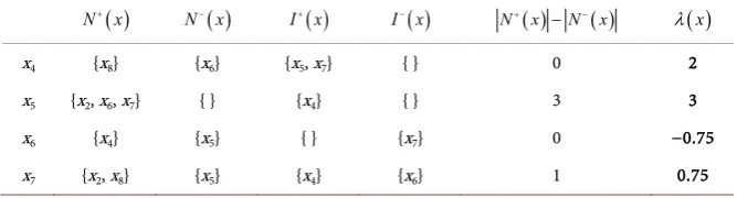
Figure 1. Example of a reduced kernel of a strongly connected component.

Table 1. Evaluating the performance of each real alternative of a strongly connected component {x4, x5, x6, x7}.

( )

N x+ _{N x}−

( )

_{I x}+

( )

_{I x}−

( )

_{N x}+( )₋_{N x}−( ) _λ

( )

_x

x4 {x8} {x6} {x5, x7} { } 0 2

x5 {x2, x6, x7} { } {x4} { } 3 3

x6 {x4} {x5} { } {x7} 0 −0.75

x7 {x2, x8} {x5} {x4} {x6} 1 0.75

subset

{

x x x x4, , ,5 6 7

}

is not a singleton whose performance (see Table 1) of

each alternative in the strongly connected component must be calculated. De-pending on the problem, one can either retain the best performer or retain only those who have a positive performance.

3.3. Using the Evolutionary Algorithm for the Problem

An evolutionary algorithm operates on a set of candidate solutions that is sub-sequently modified by two basic operators: selection and variation. Selection is used to model the reproduction mechanism among living beings, while variation mimics the natural capability of creating new living things by means of recom-bination and mutation [29]. In our proposed evolution algorithm, the selection consists in looking for the paths forming the reduced kernel of the outranking graph. This operation subdivides the current population into two subsets: the set of paths forming the reduced kernel of the outranking graph and the set of paths that do not belongs to the first subset. The crossing operator consists of selecting a path among those forming the kernel of the outranking graph and crossing it with another path. With a probability pr, this other path is chosen from the same

subset and chosen in another subset with the probability 1 − pr. The mutation

operation will consist in deleting or inserting an edge from a randomly selected kernel path. The algorithm is as follows:

1) Generate random initial population Pop with size N;

[image:8.595.206.540.292.382.2]

(9)

DOI: 10.4236/ajor.2019.93007 122 American Journal of Operations Research 3) Form a new population PopNew made up of Pop and the offspring result-ing from crossresult-ing and mutation;

4) Calculate the matrix performance of PopNew be MatPop; 5) Find the outranking graph;

6) Find the condensed outranking graph from the main outranking graph and look for its reduced kernel;

7) Form two subsets: KernelPop population from the kernel of condensed outranking graph and NotKernelPop population not belonging to KernelPop;

8) Assign Pop the population members of KernelPop or remove in Pop all population members of NotKernelPop;

9) Return Pop and stop if maximum number of generations is reached. Else consider go to Step 3.

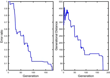
3.4. Convergence of the Algorithm

We used two performance indices [30] to measure the convergence of our mul-ti-attribute optimization method. The Error Ratio (ER) checks the proportion of non true Pareto points in the approximation front over the population size and the Generational Distance (GD) measures how far the evolved solution set is from the true Pareto front. We can observe the evolution of these two metrics in Figure 2. The algorithm is applied on a graph of 50 vertices having 734,455 paths.

4. Experiments and Results

4.1. Test Environment and Implementation

[image:9.595.173.538.449.706.2]

The programming environment used for implementation of the approach is

(10)

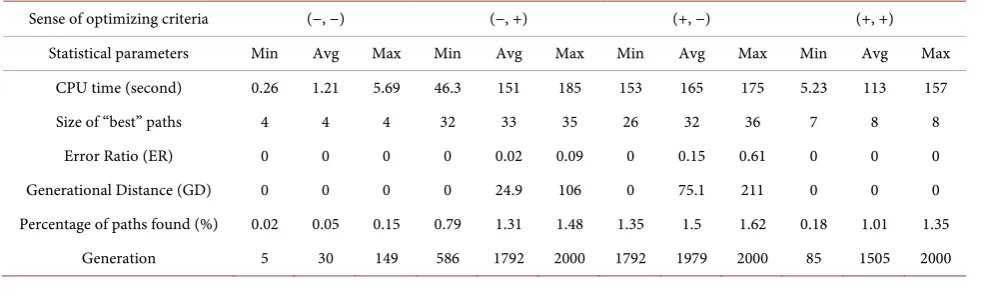
DOI:10.4236/ajor.2019.93007 123 American Journal of Operations Research MATLAB (Matrix Laboratry). All experiments were performed on a computer with a 2.3 GHz Intel(R) Core(TM) i3-2348M CPU and 4.00 GB of RAM. Three different outranking methods are implemented. Five parameters: CPU time (second), Size of “best” paths, Error Ratio (ER), Generational Distance (GD), Percentage of paths found (%) and Generation) were chosen to study the con-vergence of our method.

4.2. Tables of Results and Discussion

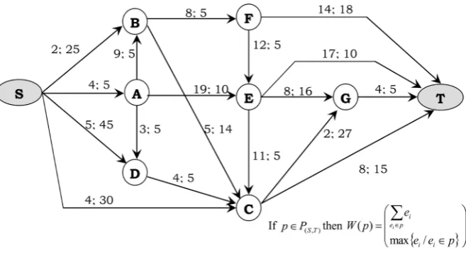
Example 1:Multi-attribute graph with nine vertices.

In Figure 3, we present a graph with two criteria to be minimized simulta-neously. The first is an additive criterion and the second is a non-additive, but a bottleneck criterion. In Figure 4, we can see the points representing the 24 paths of the graph, with the two criteria to be minimized. Among these paths, five form the reduced kernel of the outranking graph. These five paths are located on the Pareto front. The paths forming the reduced kernel are:

Path 1 (10; 30): S→_C→_G→_{T; Path 2 (15; 25): S}→_B→_C→_{T; Path 3 (13;} 27): S →_B→_C→_G→_T.

Path 4 (40; 10): S →_A→_E→_{T; Path 5 (20; 15): S}→_A→_D→_C→_T. Example 2:Multi-attribute graph with 50 vertices.

[image:10.595.211.540.531.711.2]

An acyclic graph with 50 vertices of 10% density and two attributes was ran-domly generated for simulation. The first criterion is additive, the second is a bottleneck criterion. At first, we generated all the paths in the graph. The ex-haustive search time was 9 h 20 m 10 s. The number of paths found is 734,455. The second step was the generation of Pareto-efficient paths. Table 2 shows the CPU time and size of Pareto-efficient paths. The symbol “−” (resp. “+”) means that the criterion must be minimized (resp. maximized). Thus for example (+, −) means that the first criterion is maximized while the second is minimized. Third, we ran our method and compared the “best solutions” obtained with the Pareto front. For each sense of optimizing criteria, we ran our method ten times. Tables 3-5 present the results obtained by applying our method respectively to PROMETHEE,

(11)

[image:11.595.209.541.66.416.2]

Figure 4. Different paths: the paths forming the reduced kernel located on pareto front.

Table 2. The set of Pareto solutions for exhaustive search.

Sense of optimizing criteria (−, −) (−, +) (+, −) (+, +) CPU time (m:s) 6 m 27 s 2 m 39 s 13 m 47 s 18 m 35 s Size of Pareto front 4 35 35 8

ELECTRE SPARTE methods.

In Table 3 to Table 5, we have on the first row the execution time of our al-gorithm; on the second row the number of the best solutions found; on the third and fourth rows the Error Ratio and Generational Distance performance me-trics. On the fifth row the percentage of distinct solutions found during the search for best solutions. And finally, the number of generations reached itera-tively by the genetic algorithm. On the columns, for the ten executions, we dis-play the minimum (min), the average (avg) and the maximum (max) value of each parameter.

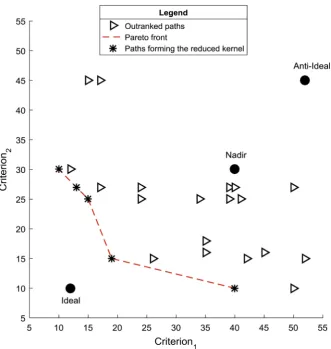
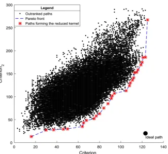
In Figure 5, we observe all the solutions forming the reduced kernel and the set of combinatorial alternatives. This is the case where the first criterion is maximized while the second criterion is minimized.

[image:11.595.206.540.464.516.2]

(12)

[image:12.595.57.543.250.388.2]

DOI:10.4236/ajor.2019.93007 125 American Journal of Operations Research (ER) and GD. However the number of solutions provided is not significant compared to the other two methods. The SPARTE and ELECTRE methods yielded similar results. In these two methods, the five observation parameters are very satisfactory. On the four senses of optimizing criteria, the SPARTE method is better in execution time. The time does not exceed 4 minutes and the error ra-tio is always very close to 0. The distance of the set of “best” solura-tions found in relation to the Pareto front is equal to 0 for the best execution cases. The per-centage of paths found never exceeded 2%. This shows that our method does not need to explore a very large number of alternatives to converge to the Pareto front.

Table 3. PROMETHEE method coupled with an evolutionary algorithm.

Sense of optimizing criteria (−, −) (−, +) (+, −) (+, +) Statistical parameters Min Avg Max Min Avg Max Min Avg Max Min Avg Max

CPU time (second) 51.7 53.1 55.5 88.5 89.5 91.2 95.3 97.4 98.9 137 144 153 Size of “best” paths 1 1 1 1 1 2 1 1 1 1 1 1

[image:12.595.57.546.418.556.2]

Error Ratio (ER) 0 0 0 0 0 0 0 0 0 0 0.4 1 Generational Distance (GD) 0 0 0 0 0 0 0 0 0 0 28.3 71.6 Percentage of paths found (%) 1.53 1.54 1.56 1 1.04 1.07 1.02 1.19 1.49 1.64 1.81 2.11 Generation 2000 2000 2000 2000 2000 2000 2000 2000 2000 2000 2000 2000

Table 4. Statistic ELECTRE1 method coupled with an evolutionary algorithm.

CPU time (second) 0.56 5.15 14.6 13.5 113 152 140 146 151 2.26 55.3 138 Size of “best” paths 4 4 4 32 34 35 28 33 35 7 8 8

Error Ratio (ER) 0 0 0 0 0.01 0.03 0 0.37 0.62 0 0.03 0.14 Generational Distance (GD) 0 0 0 0 7.4 37 0 138 210 0 14.3 71.6 Percentage of paths found (%) 0.03 0.08 0.13 0.43 1.21 1.57 1.33 1.45 1.68 0.11 0.75 1.31 Generation 16 65 137 243 1547 2000 2000 2000 2000 45 883 2000

Table 5. Statistic SPARTE method coupled with an evolutionary algorithm.

CPU time (second) 0.26 1.21 5.69 46.3 151 185 153 165 175 5.23 113 157 Size of “best” paths 4 4 4 32 33 35 26 32 36 7 8 8

Error Ratio (ER) 0 0 0 0 0.02 0.09 0 0.15 0.61 0 0 0 Generational Distance (GD) 0 0 0 0 24.9 106 0 75.1 211 0 0 0 Percentage of paths found (%) 0.02 0.05 0.15 0.79 1.31 1.48 1.35 1.5 1.62 0.18 1.01 1.35

[image:12.595.55.549.586.736.2]

(13)

[image:13.595.211.543.64.368.2]

Figure 5. Different paths: the paths forming the reduced kernel located on Pareto front.

5. Conclusions and Perspectives

In this paper, we have shown that it is possible to use the outranking methods for solving a multi-attribute combinatorial problem. This approach is based on searching for the reduced kernel of the outranking graph. Theorem 2, which we have established on the reduced kernel of induced subgraphs, has served us as an algorithmic basis. Thus, by iteratively searching for the reduced kernel of the induced subgraphs, it is possible to extract the solutions from a combinatorial optimization problem. Three outranking methods: PROMETHEE, SPARTE and ELECTRE were each coupled to an evolutionary algorithm. The resulting solu-tions were compared to the Pareto front. The results were very satisfactory for the SPARTE and ELECTRE methods compared to the PROMETHEE method.

As perspectives we intend to use this method with other metaheuristic such as simulated annealing and Taboo search, and apply it to other combinatorial op-timization problems like Minimum Spanning Tree Problem multi-attributes that have real applications in the network coverage domain.

Conflicts of Interest

The authors declare no conflicts of interest regarding the publication of this paper.

References

(14)

Opera-DOI:10.4236/ajor.2019.93007 127 American Journal of Operations Research tional Research, 45, 324-331.https://doi.org/10.1016/0377-2217(90)90196-I

[2] Valerie, B. (1990) Multiple Criteria Decision Analysis: Practically the Only Way to Choose. University of Strathclyde, Glasgow.

[3] Florent, J., Thériault, M. and Musy, A. (2001) Using GIS and Outranking Multicri-teria Analysis for Land-Use Suitability Assessment. International Journal of Geo-graphical Information Science, 15, 153-174.

https://doi.org/10.1080/13658810051030487

[4] Kepaptsoglou, K., Karlaftis, M.G. and Gkountis, J. (2013) A Fuzzy AHP Model for Assessing the Condition of Metro Stations. KSCE Journal of Civil Engineering, 17, 1109-1116.https://doi.org/10.1007/s12205-013-0411-0

[5] Marinoni, O. (2006) A Discussion on the Computational Limitations of Outranking Methods for Land-Use Suitability Assessment. International Journal of Geographi-cal Information Science, 20, 69-87.https://doi.org/10.1080/13658810500287040 [6] Eastman, J.R., Kyem, P.A.K. and Toledano, J. (1993) A Procedure for

Mul-ti-Objective Decision Making in GIS under Conditions of Conflicting Objectives. Proceedings of the 4th European Conference on Geographic Information Systems, EGIS’93 (Utrecht: EGIS Foundation), 438–448.

[7] jankowski, P., Nyerges, T.L., Smith, A., Moore, T.J. and Horvath, E. (1997) Spatial Group Choice: A SDSS Tool for Collaborative Spatial Decisionmaking. Internation-al JournInternation-al of GeographicInternation-al Information Science, 11, 577-602.

https://doi.org/10.1080/136588197242202

[8] Pereira, J.M.C. and Duckstein, L. (1993) A Multiple Criteria Decision-Making Ap-proach to GIS-Based Land Suitability Evaluation. International Journal of Geo-graphical Information Science, 7, 407-424.

https://doi.org/10.1080/02693799308901971

[9] Grabisch, M. (2005) Une approche constructive de la décision multicritère. Traite-ment du signal, 22, 321-337.

[10] Dammak, F., Baccour, L. and Alimi, A.M. (2016) Crisp Multi-Criteria Decision Making Methods: State of the Art. International Journal of Computer Science and Information Security, 14, 252.

[11] Hwang, C.-L. and Yoon, K. (1981) Methods for Multiple Attribute Decision Mak-ing. In: Multiple Attribute Decision MakMak-ing. Lecture Notes in Economics and Ma-thematical Systems, Springer, Berlin, Heidelberg, 58-191.

https://doi.org/10.1007/978-3-642-48318-9_3

[12] Benayoun, R., Roy, B. and Sussman, B. (1966) Electre: Une méthode pour guider le choix en présence de points de vue multiples. Note de travail, 49.

[13] Roy, Bernard. (1968) Classement et choix en présence de points de vue multiples. Revue française d’informatique et de recherche opérationnelle, 2, 57-75.

https://doi.org/10.1051/ro/196802V100571

[14] Brans, J.P., Mareschal, B. and Vincke, P. (1978) A New Family of Outranking Me-thods in Multi-Criteria Analysis. Cahiers du Centre d’études de Recherche Opéra-tionnelle, 3-24.

[15] Neumann, J.V.,Morgenstern, O., Kuhn, H.W. and Rubinstein, A. (2007) Theory of Games and Economic Behavior.Princeton University Press, Princeton, NJ.

[16] Kalyanmoy, D. (2014) Multi-Objective Optimization. In: Burke, E. and Kendall, G., Eds., Search Methodologies, Springer, Boston, MA, 403-449.

https://doi.org/10.1007/978-1-4614-6940-7_15

(15)

DOI: 10.4236/ajor.2019.93007 128 American Journal of Operations Research Np-Completeness. Revista Da Escola De Enfermagem Da USP, 44, 340.

[18] He, F., Huan, Q. and Qiong, F. (2007) An Evolutionary Algorithm for the Mul-ti-Objective Shortest Path Problem. Proceedings of the International Conference on Intelligent Systems and Knowledge Engineering (2007), ISKE 2007, Chengdu 15-16 October 2007. https://doi.org/10.2991/iske.2007.217

[19] Pangilinan, J.M.A. and Gerrit, J. (2007) Evolutionary Algorithms for the Mul-ti-Objective Shortest Path Problem.Int J Appl Sci Eng Technol, 4, 205-210.

[20] Greco, S., Figueira, J.R. and Ehrgott, M. (2016) Multiple Criteria Decision Analysis. Springer, New York.https://doi.org/10.1007/978-1-4939-3094-4

[21] Fustier, B. (1981) Une méthode d’analyse multicritère SPARTE. Diss. Institut de mathématiques économiques (IME).

[22] Jørgen, B.-J. and Gutin, G.Z. (2008) Digraphs: Theory, Algorithms and Applica-tions. Springer Science & Business Media, ‎Berlin‎/‎Heidelberg.

[23] Tzeng, G.-H. and Huang, J.-J. (2011) Multiple Attribute Decision Making: Methods and Applications.Springer-Verlag,New York.https://doi.org/10.1201/b11032 [24] Richardson, M. (1953) Solutions of Irreflexive Relations. Annals of Mathematics,

58, 573-590.https://doi.org/10.2307/1969755

[25] Fraenkel, A.S. (1981) Planar Kernel and Grundy with d≤ 3, dout≤ 2, din≤ 2 Are NP-Complete. Discrete Applied Mathematics, 3, 257-262.

https://doi.org/10.1016/0166-218X(81)90003-2

[26] Sharir, M. (1981) A Strong-Connectivity Algorithm and Its Applications in Data Flow Analysis. Computers & Mathematics with Applications, 7, 67-72.

https://doi.org/10.1016/0898-1221(81)90008-0

[27] Chen, R. and Jean-Jacques, L. (2017) Une preuve formelle de l’algorithme de Tar-jan-1972 pour trouver les composantes fortement connexes dans un graphe. JFLA 2017-Vingt-huitièmes Journées Francophones des Langages Applicatifs.

[28] Ruohonen, K. (2013) Graph Theory.

[29] Zhou, A., et al. (2011) Multiobjective Evolutionary Algorithms: A Survey of the State of the Art. Swarm and Evolutionary Computation, 1, 32-49.

https://doi.org/10.1016/j.swevo.2011.03.001

[30] Van Veldhuizen, D.A. and Lamont, G.B. (2000) Multiobjective Evolutionary Algo-rithms: Analyzing the State-of-the-Art. Evolutionary Computation, 8, 125-147.