Intelligent Evidence-Based Management for Data
Collection and Decision-Making Using Algorithmic
Randomness and Active Learning
Harry Wechsler1, Shen-Shyang Ho2
1George Mason University, Fairfax, USA
2University of Maryland, College Park, Maryland, USA
E-mail: [email protected], [email protected]
Received April 13, 2011; revised April 28, 2011; accepted May 10, 2011
Abstract
We describe here a comprehensive framework for intelligent information management (IIM) of data collec-tion and decision-making accollec-tions for reliable and robust event processing and recognicollec-tion. This is driven by algorithmic information theory (AIT), in general, and algorithmic randomness and Kolmogorov complexity (KC), in particular. The processing and recognition tasks addressed include data discrimination and multi-la- yer open set data categorization, change detection, data aggregation, clustering and data segmentation, data selection and link analysis, data cleaning and data revision, and prediction and identification of critical states. The unifying theme throughout the paper is that of “compression entails comprehension”, which is realized using the interrelated concepts of randomness vs. regularity and Kolmogorov complexity. The constructive and all encompassing active learning (AL) methodology, which mediates and supports the above theme, is context-driven and takes advantage of statistical learning, in general, and semi-supervised learning and transduction, in particular. Active learning employs explore and exploit actions characteristic of closed-loop control for evidence accumulation in order to revise its prediction models and to reduce uncertainty. The set-based similarity scores, driven by algorithmic randomness and Kolmogorov complexity, employ strangeness/typicality and p-values. We propose the application of the IIM framework to critical states pre-diction for complex physical systems; in particular, the prepre-diction of cyclone genesis and intensification.
Keywords:Active Learning, Algorithmic Information Theory, Algorithmic Randomness, Evidence-Based
Management, Kolmogorov Complexity, P-Values, Transduction, Critical States Prediction
1. Introduction
Information loaded with meaning and in context is an asset and is referred throughout this paper as evidence. Intelligent evidence-based management (EBM) of data concerns the value-added to raw data in order to trans-form it into (referential) intrans-formation and (meaningful) knowledge using purposeful action (DKA). The motiva-tion for EBM comes from Microsoft (MS) Cambridge (UK) Research manifesto Towards 2020 Science [1]. First and foremost the manifesto notes that what will most likely have a profound impact is “the leap from support to ‘do’ science, i.e., computational science, to the integration of computing into the very fabric of science” leading to science-based innovation. The MS report highlights that an immediate and important challenge is
fur-ther traced to the “schemata” (kind of meaningful knowledge) proposed by Neisser [2] to account for the perceptual cycle where available information modifies the schema, the schema then directing then exploration, and exploration then sampling information. The outcome of the explorations—the information picked up-modifies the original schema. The Perception-Control-Action-Lea- rning (PCAL) proposed by Wechsler [3] has expanded on the schema framework to include anticipation and learning driven by exploration and exploitation, which are mediated by control and action/manipulation.
This paper advances a comprehensive framework for EBM using DKA, which is concerned with data collec-tion and decision-making related accollec-tions for reliable and robust event prediction and recognition. Data collection includes among others data aggregation, data cleaning, data collection, data selection, and data segmentation. Reliability concerns consistency and stability of the pre-dictions made, while robustness is about coping with adversarial information, e.g., incomplete and corrupt information. The motivation for this paper comes from apparent synergies between information theory (IT) [4], algorithmic information theory [5,6], Kolmogorov Com-plexity [6,7] (see Section 6 and 7), statistical learning theory (SLT) [8], and algorithmic learning [9].
(Algo-rithmic information theory is a subfield of HHHHH
HHHHH and HHHHH
relationship between HHHHHHHHHHHHHHH.) The
unifying theme throughout is that of “compression en-tails comprehension”, which is realized using the inter-related concepts of randomness opposite regularity, Kolmogorov complexity, and minimum description length (MDL). The constructive active learning interface, which mediates and supports the above theme, is con-text-driven and takes advantage of semi-supervised learning [10] and transduction [8]. Active learning [11] is first and foremost about the choices made during data collection. It employs explore and exploit actions char-acteristic of closed-loop control for evidence accumula-tion in order to reduce uncertainty and to revise the pre-diction models. The event-recognition tasks addressed
i n c l u d e m u l t i -
layer data categorization, change detection, data cleaning and data revision, data fusion, data segmentation, data selection and link analysis, and prediction and identifica-tion of critical states.
The basic functionalities active learning supports in-clude decisions on where to explore and what (labeled and unlabeled) data to gainfully employ for further ad-aptation and modeling purposes; on how to process and fuse the information and knowledge acquired; on han-dling time-varying data streams, detecting change, and choosing when to revise the prediction models. Towards that end, set-based similarity scores are proposed. They
are motivated by KC and driven by strangeness/typicality and p-values. The scores take advantage of associations, context and relationships; cohorts and rankings; trans-formations, e.g., hints and perturbations, censoring and imputation (to account for missing information), and data cleaning and revision (for consistency, error correction, and stability). Note that the terminology used in this pa-per employs similarity scores to estimate proximity. The use of “metrics” and “distances” is avoided, and the con-text makes clear when strict definitions are used.
The outline for the paper is as follows. EBM and DKA are discussed in Section 2 Active Learning; Algorithmic Information Theory and Closed-Loop Control; discrimi-native methods and practical intelligence; Kolmogorov complexity; and algorithmic randomness are discussed in Sections 3 -7, respectively. Strangeness/typicality and p-values; transduction and semi-supervised learning; and multi-layer and multi-set open set categorization are dis-cussed in Sections 8 - 10 Active learning (see Section 3) using the explore and exploit paradigm motivates and supports functionalities related to data collection and evidence accumulation. The specific functionalities, concerning change detection; data aggregation/data fu-sion; data selection and link analysis; data cleaning and data revision; and prediction and identification of critical states, are described in Sections 11 - 16, respectively. New dimensions and requirements on EBM and DKA, e.g., for life sciences, are discussed in Section 17 The paper concludes in Section 18 with a brief summary and venues for future research.
2. Evidence-Based Management: From Data
to Knowledge to Action
Evidence is any data or information so given, whether collected or derived from any source. Management is meant here to denote (organizational) activities pursued to accomplish desired goals and objectives related to data collection and assimilation in an efficient and effective
fashion. For all purpose, management compHHHHH
HHHHH
purposes, surrounds recognition, where the primary task is that of multi-layered open set categorization to per-form (unlabelled) data annotation and revision. Knowl-edge amounts to the models learned and relearned (“re-vised”) in order to make consistent and stable predictions mostly on detection, classification, and discrimination.
Knowledge discovery is about modeling the environ-ment for the purpose of reliable and robust prediction. Reliability in terms of consistency (in the limit) and sta-bility of the predictions made, and robustness for dealing with incomplete and corrupt (adversarial) data sources and actions. The knowledge discovered is tasked to fa-cilitate, guide, and support decision-making. EBM and DKA expand first on intelligent information manage-ment (IIM) [12], with the latter limited to a life—cycle of data creation, acquisition, organization, storage, retrieval, dissemination and sharing, and use, but devoid of adap-tation and knowledge discovery. EBM and DKA expand also on knowledge management (KM) [13,14], with the latter assuming that much of knowledge already exists but devoid of the critical adaptive exploration and ex-ploitation cycles, which are geared to further knowledge discovery and knowledge betterment. KM merely com-prises a range of strategies and practices used (in an or-ganization) to identify, create, represent, distribute, and
enable adoption of HHHHHHHHHH and HHHHH
knowledge is already available and needs only to be em-bedded for practical uses.
EBM and DKA involve for all practical purposes suc-cessive hypothetical-deductive cycles of discovery, whe- re an initial predictive model learned from data guides the iterative collection of new data, model revision with new hypotheses/inferences (“labeling”) made on unla-beled data, and so on. Examples of such revisions for signal tracking and interpretation include Sequential Monte Carlo (SMC) methods/Sequential Importance Sampling (SIS) also known as particle filtering [15]. The more complex active learning process described later also includes (a) change and anomaly (outlier, surprise, large and extreme values) detection; (b) data perturba-tions, synthesis, and class membership revisions (caused by possible errors in annotation), with the latter including filling in for missing data using anticipation, censoring and imputation, and/or proactive learning; and (c) mixed modes of adaptation using co-training, transfer learning, and/or multi-task learning for optimal resource-bounded data collection. Towards that end, EBM and DKA have access to multi-set (of instances) similarity scores, which take further advantage of associations, context, and rela-tions.
3. Active Learning
One can approach EBM and DKA in terms of
(progres-sive) evidence accumulation from time-varying data streams for the purpose of data collection, reasoning (“prediction”), and adaptation. This view related to ac-tive learning is engaged in data compression while it filters, fills in, and summarizes data contents. Active learning seeks for the patterns most responsible to gener-ate and model the data, while always on look to detect when the data generation models change and to choose the means and ways to best process the data. Active learning is all encompassing, including autonomic com-puting [16] and W5+. Autonomic comcom-puting, also re-ferred to as self-management, is about closed-loop control. It provides basic functionalities, e.g., self-configureura- tion (for planning and organization), self-optimization (for efficacy), self-protection (for security purposes), and self-healing (to repair malfunctions).
W5+ answers questions related to What data to con-sider, When to get/capture the data and from Where, and How to best process the data. An additional Who (is) question about identity becomes relevant to biometrics and identity management. Consider now intelligence an- alysis where directed evidence accumulation should also consider and document the explanation Why dimension. The Why dimension interrelates observations and hy-potheses (models) duly ascribed (abducted possibly us-ing analogy reasonus-ing, Bayesian (belief) networks [17], and/or causality [18]) and expectations to be met. The Bayesian networks (for inference and validation pur-poses) assist with optimal and incremental/progressive intelligence data collection. In a fashion similar to signal processing and transmission, the “progressive” aspect signifies incremental access and/or display of crucial evidence, which at some point is enough to solve the puzzle and/or make recognition apparent.
bet-ter attention and selectivity, focus, anticipation, and im-proved forecasts.
Everything about active learning is data centric. It is also about on-line learning and prediction with the pur-pose of data analytics for streaming data. Active learning is further sensitive to change and drift, which suggests that a time-varying D(t)K(t)A(t) model, indexed by time t, needs to supplant DKA in support of EBM. Towards that end, active learning considers associations, context, granularity, relationship, and space x time domains; lev-erages local and global context, on one side, and central and distributed processing, on the other side; and last but not least it involves multi—strategy learning.
4. Algorithmic Information Theory and
Closed-Loop Control
The medium that facilitates EBM using DKA takes ad-vantage of Algorithmic Information Theory and Closed- Loop Control (CLC). The starting point for this medium is Information Theory, which is about storage and commu-nication, in general, and capacity, compression, accuracy, rate-distortion, and error correction, in particular. Algo-rithmic Information Theory provides for information processing, in general, and algorithmic issues related to the interrelated aspects of compression and prediction, in particular. Algorithmic Information Theory, throughout this paper, is about compressibility and generalization for the purpose of learning. The better some model or theory can compress training (“learning”) data, the better the generalization achieved is, and the more effective, reliable, and robust the prediction ability becomes. This conforms with the dictum enunciated by Leibniz that “comprehen-sion entails compres“comprehen-sion,” and is conceptually similar to the MDL inductive principle, which gives support to dis-criminative methods for recognition (see Section 5). AIT, in general, and KC, in particular (see Sections 6 and 7) are related to CLC in terms of “universal prediction” [5] using statistical learning and similarity scores. Solid relations, related to accuracy performance, can be further established between information theory and statistical learning theory [19] to enhance modeling and prediction.
Prediction requires adaptation and learning, with the latter denoting “changes in the system that are adaptive in the sense that they enable the system to do the same tasks drawn from the “same” population more efficiently the next time” [20]. Learning is by default incremental and on-line learning should be preferred to batch learn-ing (see Section 15). Note that learnlearn-ing plays a funda-mental role in facilitating “the balance between internal representations and external regularities” [21], with CLC responsible for purposeful and successful action and
be-havior. One can thus connect IT, AIT, and CLC in terms of technical performance (“efficacy”), meaning and se-mantics, and action and behavior (“effectiveness”).
CLC is also about causation, feedback, and change. Similar to cybernetics, which has been characterized by
HHHHH as “the art of ensuring the efficacy
of action”, CLC can be approached as the
interdiscipli-nary study of autonomous HHHHHHHHHH (see Section
3 for the self-management aspect of active learning). It comes to the fore when an action causes some change in the environment and that change becomes manifest to the system via information, or feedback, which then causes the system to adapt to new conditions. CLC participates HHHHH, which transition from action
to exploratory sensing (“data collection”); modeling (for exploitation), prediction and evaluation, and again to (sensory) action. This is the very epitome for DKA. Sen-sory action is much more than merely data collection. It also involves (internal) perturbations of the data available (both labels and representation) and subsequent revision of current models (see Section 15). The challenges CLC faces are twofold, behavior effectiveness subject to effi-ciency in terms of the resources used, and proper structure and organization for the control system responsible for the displayed behavior. This requires among others con-text and self-organization using clustering.
Action and adaptation are primordial and most impor-tant for CLC. They are interrelated using the observer, structural couplings, and “breaking down” and “throw-ness” aspects of behavior-based and grounded intelligence. These are mere reflections of feedback, context, and proper generalization, with practical understanding being more fundamental than detached theoretical understanding (see Section 5). Context includes intricate relationships between understanding and existing ontologies [22]. Along the same lines, Heidegger [22] “insists that it is meaningless to talk about the existence of objects [knowl-edge] and their properties in the absence of concernful activity, with its potential for breaking down” [wrong pre-dictions]. Closed-loop control supports both meaningful action and adaptation, and involves iterative explore and exploit cycles across the data landscape. Furthermore, the goal for predictive learning is behavior-based imitation (of the unknown data model) rather than its identification. The inductive principle, e.g., transduction (see Section 9), is responsible for the particular model selected and it directly affects the generalization ability in terms of prediction risk, i.e., the performance on unseen/future (unlabeled test) data. This is the main reason to prefer discriminative rather than (normative) generative (prescriptive) methods. Discrimi-native methods are discussed next.
Intelligence
Discriminative methods support practical intelligence, in general, and inference and prediction, in particular, for the purpose of discrimination. Progressive processing, (trans-formational and integrative) evidence accumulation, like-lihood ratios (LR) and odds, and fast decision-making are the hallmark of practical intelligence. There is no time for expensive density estimation and marginalization, which are characteristic of generative methods (see below). This together with apparent relationships between discrimina-tive methods and Kolmogorov complexity (see Section 6 and 7) are the motivation behind the similarity scores proposed throughout this paper for the purpose of catego-rization and recognition. Discriminative methods seek for non-accidental coincidences and take advantage of in-fomax and sparse codes for association [23].
Formally, “the goal of pattern classification can be approached from two points of view: informative [gen-erative]—where one learns the class densities, e.g., HMM, or discriminative—where the focus is on learning the class boundaries without regard to the underlying class densities, e.g., logistic regression and neural net-works” [24]. The generative methods, normative and prescriptive in nature, synthesize the classifier by learn-ing what appear to be the specific class distributions, and make their decisions using maximum a-posteriori prob-ability (MAP). The discriminative methods imitate and model only what it takes to make the classification effec-tive. The discriminative methods are in tune with both structural risk minimization [8] and transduction (see Section 9). They are aligned with structural risk minimi-zation (SRM) because they lock on what is essential for discrimination, and they are aligned with transduction because discrimination implements local (cohort) esti-mation. Jebara [25] has actually suggested that imitation should be added to the generative and discriminative methods as another model for learning and reasoning. Jebara recalls from Edmund Burke that “it is by imitation, far more than by percept, that we learn everything.” Dis-criminative methods make fewer assumptions and fewer assumptions mean less chance to make mistakes.
Discriminative methods avoid estimating how the data has been generated and instead focus on estimating the posteriors (for recognition) in a fashion similar to the use of likelihood ratios (LR) and odds. The informative ap-proach for 0/1 loss assigns some input x to the class k ε K for which the class posterior probability P (y = k | x) yields the maximum. The MAP decision used by genera-tive methods requires instead access to the log-likelihood Pθ(x, y). The optimal (hyper) parameters θare learned
using maximum likelihood (ML) and a decision bound-ary is then derived, which corresponds to a minimum
distance classifier. The discriminative approach models directly the conditional log-likelihood or posteriors Pθ(y |
x). The optimal parameters are estimated using ML leading to the discriminative function,
log
k
P y k x x
P y K x
which is similar in use to the Universal Background Model (UBM) for similarity score normalization and/or LR definition. The comparison takes place between some specific class membership k and a generic distribution
(over K) that describes everything known about the
population at large. The discriminative approach has been found [24] to be more flexible and robust compared to informative/generative methods because fewer as-sumptions need to be made.
6. Kolmogorov Complexity
The Kolmogorov complexity K (x) of a finite string x is the information in x defined by the length of the shortest program for a reference Universal Turing Machine (en-coded in binary bits) that outputs the string x [6]. Infor-mation distance d (x, y) is the length of the shortest pro-gram on the reference Universal Turing Machine com-puting y from x and x from y. It has been proven that up to an additive logarithmic term, d (x, y) = max {K (x | y), K (y | x)} [26] where K (x | y) is the conditional complex-ity of x given y. The normalized information distance (NID) between two strings x and y is formally defined as
, max
,
,
max ,
K x y K y x NID x y
K x K y
with K (x) (and K (y)) approximated by a real-life
com-pressor C such that C (x) is the length of the compressed version of x [6].
7. Algorithmic Randomness
Let x be a binary string belonging to set S. K (x | S) is the Kolmogorov complexity of x given S. The randomness deficiency D (x | S) for x given S is D (x | S) = log |S| – K
(x | S) [6]. The larger the randomness deficiency is the
more regular and more probable the string x is. Kolmo-gorov complexity and randomness are conceptually re-lated through the minimum description length. As an example, transduction (see Section 9), for the purpose of categorization (see Section 10), would choose from all possible labeling (“identities”) for (unlabeled) test data the one that yields the largest randomness deficiency, i.e., the most probable labeling. Randomness deficiency is, however, not computable [6]. One has to approximate it
instead, using a slightly modified Martin—Löf test for
randomness, and the values taken by such randomness tests are called p-values. The p-value construction used (see Section 8) has been proposed by Vovk et al. [9] and Predrou et al. [27]. This is discussed next.
8. Strangeness and P-Values
Strangeness and typicality [28] [29] are interchangeable.
Given a sequence of similarity distances from sample
(instance) j to other samples l, the strangeness αj (or
al-ternatively the typicality) of j with putative label y is defined as:
1 1
k y jl l j k y
jl l
d d
The strangeness measures the lack of typicality with respect to its true or putative (assumed) identity label y
U
andU the labels for all the other exemplar patterns.
For-mally, the strangeness αj is the (likelihood) ratio (LR) of
the sum of the k nearest neighbor (k-NN) similarity (Euclidean) distances d for sample j from the same class y divided by the sum of the k nearest neighbor similarity distances for sample j from UallU the other classes (¬y).
Note that other similarity distances, e.g., Mahalanobis, could readily and effectively substitute for the Euclidean distance. The smaller the strangeness, the larger its typi-cality and the more probable its (putative) label y is. The strangeness facilitates both feature selection (similar to Markov blankets) and variable selection (dimensionality reduction) for recognition purposes. An alternative (co-hort) definition for strangeness would tabulate distances only for the most prevalent class surrounding y given the putative assignment ¬y. One finds empirically that the strangeness, classification margin, sample and hypothesis margin, posteriors, and odds are all related via a mono-tonically non-decreasing function with a small strange-ness amounting to a large margin. The margin of a
hy-pothesis with respect to an instance is the distance be-tween the hypothesis and the closest hypothesis that as-signs an alternative label to that instance. An alternative definition [30] for the hypothesis margin, similar to the strangeness definition proposed above, is
x
x nearmiss x
x nearhit x
with nearhit (x) and nearmiss (x) being the nearest sam-ples of x that carry the same and a different label, respec-tively. The strangeness can also be defined using the Lagrange multipliers associated with (kernel) SVM clas-sifiers but this requires a significant increase in computa-tion.
The use of the strangeness gets further support from the Cover-Hart theorem [31], which proves that asymp-totically the generalization error for the nearest neighbor classifier exceeds by at most twice the generalization error of the Bayes optimal classification rule. The same theorem also shows that the k-NN error approaches the Bayes error (with factor 1) if k = O (log n). The optimal piecewise linear discrimination boundary includes those
samples for whom the strangeness α is constant, i.e., α =
1 for the case of two class (“binary”) discrimination. The advantage for the strangeness k-NN against standard lazy k-NN classification is most apparent for overlapping dis-tributions. One can empirically find that the boundaries induced by the strangeness k-NN are smoother and closer to the optimal boundary compared to the boundary in-duced by k-NN, while the corresponding errors and their standard deviations are also lower.
Additional relations that link the strangeness and the Bayesian approach using the likelihood ratio can be ob-served, e.g., the logit of the probability is the logarithm of the odds, logit (p) = log (p/(1 – p)), the difference be-tween the logits of two probabilities is the logarithm of the odds ratio, i.e.,
(1 )
log
(1 )
p p
q q
= logit (p) – logit (q)
(see also logistic regression and the Kullback-Leibler (KL) divergence). Note that the logit function is the in-verse of the “sigmoid” or “logistic” function. Another relevant observation that buttresses the use of the strangeness comes from the fact that unbiased learning of Bayes classifiers is impractical due to the large number of parameters that have to be estimated. The alternative to the unbiased Bayes classifier is logistic regression, which implements the equivalent of a discriminative classifier.
statistics but are not the same [32]. The p-values are de-termined according to the relative rankings of putative authentications made against each one of the identity classes known. The standard p-value construction shown below, where l is the cardinality of the training set T, constitutes a valid randomness (deficiency) test ap-proximation [33] for some putative label y hypothesis assigned to an unlabeled new sample
#
:
1
y j new y
j p e
l
The p-values are used to assess the extent to which data supports or discredits the null hypothesis H0 (for some specific classification attempt). When the null hy-pothesis is rejected for each of the classes known, one declares that the test (“query”) pattern is “unfamiliar” as it fails to “mate” against all the known classes. The query is thus answered with “none of the above.” This corre-sponds in the case of biometrics to forensic exclusion with rejection, and it is characteristic of open set recog-nition. This is different from closed set recognition where the top choice is the default answer.
9. Transduction
Transduction is different from inductive inference. It is local inference (“estimation”) that moves from particu-lar(s) to particuparticu-lar(s). In contrast to inductive inference, where one uses empirical data to approximate a func-tional dependency (the inductive step [that moves from particular to general] and then uses the dependency learned to evaluate the values of the function at points of interest (the deductive step [that moves from general to particular]), one now infers directly (using transduction) the values of the function only at points of interest [8]. Inference now takes place using both labeled and unla-beled data, which play complementary roles to each other. Transduction incorporates unlabeled data, charac-teristic of test (“unlabeled”) samples, in the decision-ma- king process responsible for their labeling (“prediction”), while seeking for a consistent and stable labeling across both (near-by) training (“labeled data”) and test (“unla-beled”) data [34]. Transduction “works because the test set provides a nontrivial factorization of the [discrimina-tion] function class” [10].
One key concept behind transduction (and consistency) is the symmetrization lemma [8], which replaces the true (inference) risk by an estimate computed on an inde-pendent set of data, e.g., unlabeled/test data, referred to as ‘virtual’ or ‘ghost samples’. We expand on the con-cept of ghost samples to include guided perturbations and hints in order to broaden the pool of data available for learning and improve on generalization (see Section
15). Revision of the putative class (“label”) assignments drives the process responsible with determining (“infer-ring”) the appropriate rejection threshold for multi-layer categorization, in general, and open set recognition, in particular (see Section 10).Transduction seeks consistent labels for both training and test data. It iterates to relabel the test data using local perturbations on the labels al-ready assigned. Poggio et al. [35], using similar reason-ing, suggest it is the stability of the learning process that leads to good predictions. In particular, the stability property says that “when the training set is perturbed by deleting one example, the learned hypothesis does not change much. This stability property stipulates condi-tions on the learning map rather than on the hypothesis space.” Integral to revision, the concept of stability is expanded to allow for both label changes and training samples deletion (see Section 15). This learning ap-proach can be further analyzed using regularization [36]. The goal for inductive learning is to generalize for any future test set, while the goal for transductive inference is to make predictions for some specific/given working set W. Test data is not merely a passive collection of data waiting for labeling but rather an active player ready to add its own contribution to that provided by the labeled training data. The working or test samples provide addi-tional information about the underlying data distribution and their explicit inclusion in the problem formulation yields better generalization on problems with insufficient labeled points [9]. Transductive inference therefore seeks to find, from all possible labeling L (classifications) L (W) for working (unlabeled) test data set W, the one that yields the largest randomness deficiency, i.e., the most probable labeling. This choice models the working (“test”) sample set W in a fashion similar to that used for the training set T. Towards that end, transduction has to minimally change the original model learned for T. “The difference between the classifications that induction and transduction yield for some working sample approxi-mates its randomness deficiency. As one disturbs a clas-sifier (driven by T) using working but putatively labeled samples to augment the training set, the magnitude of the disturbance estimates the classifier’s instability (unreli-ability) in a given region of its problem space. Similar and complementary to transduction is semi-supervised learning (SSL) [10] (see Section 14).
10. Multi-Layer and Multi-Set Open Set
Data Categorization
(“bin-inng”). Open set recognition operates under the assumption that some of the unlabeled patterns asking for recognition are unknown (unfamiliar) and can’t be recognized. This is addressed by making available a reject (“unknown”) answer. Given an unlabeled (pattern)
exemplar e, the corresponding p-values, for each
puta-tive label (class) drawn from training data, record the likelihood that the new pattern belongs to that putative class. If some p-value p is high enough and it signifi-cantly outscores the others, the new pattern can be mated to the corresponding class with credibility p. If the top ranked (highest p-values) choices are very close to each other but outscore the other choices, the top ranked label choice is credible but ambiguous in its classification, and should thus carry a low confidence during further processing. The confidence measures the difference between the first and second largest (or con-secutive) p-values. If all p-values are randomly distrib-uted and no p-value significantly outscores the other p-values, any choice of labels is questionable and the new exemplar can’t be recognized and should be thus rejected. The credibility and confidence indexes/simil- arity scores are useful for data fusion purposes (see Sec-tion 13).
The implementation details regarding open set deci-sion-making are generic as they apply to each categori-zation layer. One re-labels the training patterns, one at a time, with all possible putative labels except the ground truth originally assigned to it. As an example, detection involves just two labels. The peak-to-side (PSR) ratio, PSR = (pmax – pmin)/pstdev, traces the characteristics of the
resulting p-value distribution and determines, using cross validation, the [a priori] threshold needed for open-set recognition. The PSR values found for un-known patterns are low because they do not mate; their relative strangeness is high, and their p-values low. As an example, imagine unknown (unlabeled) exemplars as impostors when recognition concerns biometrics. Im-postors should be deemed as outliers and be thus re-jected as unknown (“none of the above”) vis-à-vis the labels (identities) known (enrolled) [37]. The open set recognition approach just described provides for both reliability and robustness. Reliability in terns of consis-tency and stability of learning, while robustness vis-à- vis incomplete and corrupt information. The same ap-proach renders itself suitable for both anomaly and/or outlier detection.
Training data consists of (x, y) patterns, where x stands for representation, and y stands for the pattern label (class). The similarity scores discussed so far assumed that each class (“set”) consists of only one pattern. This assumption does not hold in the general case when mul-tiple instances can account for variability, increase the
signal-to-noise ratio, and provide for better generaliza-tion. Towards that end, the Hausdorff distance substitutes for the Euclidean distance d used to define the
strange-ness (see Section 8) leading to the multi-set distance dH
for sets A and B
,
max sup inf
, ,sup inf
,
u b B a A
a A b B
d A B d a b d a b
There are other ways to define multi-set similarity scores. As an example, similarity can be defined by the
angle between the subspace SB of unlabeled patterns (set
B) and the subspace SAof reference (labeled) training
pattern (set A). The subspaces SA and SB are estimated
(learned) possibly as eigenspaces. Alternatively, one can learn the subspaces on Grassman manifolds and employ principal angles, Binet-Cauchy and Procrustes metrics for similarity distances [38]. The assumption still holds that both sets A and B are multi-sets consisting of in-stances coming from only one class. We relax this as-sumption (see Section 14) when we allow multi-sets A
and B whose instances can come from more than one
class. The scope for categorization expands using boost-ing and transduction for data aggregation (see Section 13) and both qualitative and quantitative similarity scores (see Section 18).
Active learning (see Section 3) is context-driven and takes advantage of statistical learning, in general, and transduction and semi-supervised learning, in particular, to provide for additional event-recognition functionalities. Active learning employs explore and exploit actions characteristic of closed-loop control for evidence accu-mulation in order to revise its prediction models and to reduce uncertainty. Continuous interactions with the en-vironment provide the feedback necessary to iterate on EBM and DKA. Towards that end, algorithmic informa-tion theory, algorithmic randomness, and closed-loop control collaborate to advance intelligent data collection, knowledge (“model”) discovery (“extraction”), and pur-poseful behavior (“action”). This is discussed over the next sections (see Sections 11 - 16). It is helpful to note that, according to Maturana, “learning is not [merely] a process of accumulation of representations of the envi-ronment; it is a continuous process of transformation of behavior through continuous change in the capacity of the nervous system to synthesize [and incorporate] it’ [22].
The multi-set based similarity scores proposed are all driven by algorithmic randomness and Kolmogorov complexity. Additional similarity scores are described in order to expand on strangeness/typicality and p-values, while taking advantage of associations, context and rela-tionships for the purpose of link analysis and selection (see Section 14). Metrics are also made available for data cleaning and data revision, e.g., label editing (to account for annotation errors) and censoring and imputation (to fill in for missing data), on one side, and appearance perturbations and synthesis (for consistency and stability) (see Section 15). Finally, we address yet another func-tionality, that of criticality identification and prediction, which belongs to complex system identification and pre-diction (see Section 16). The latter functionality is an example where the interplay between similarity scores (see Section 8) and change detection (see Section 12) shows how more complex behavior can emerge.
11. Data Collection and Evidence
Accumulation
Active learning is concerned with evidence accumulation (“data sampling and collection”) towards choosing the most (functionally) relevant examples to improve the classification (“margin”) for both effectiveness (“accu-racy”) and efficiency (“number of examples needed”). The active learning solution proposed here is driven by transduction and it is realized using strangeness and p-values [32]. The p-values provide a measure of diver-sity and disagreement in opinion regarding the true label of an unlabeled example when it is assigned all possible putative labels. Let pi be the p-values obtained for a
par-ticular example xn+1 using all possible labels i = 1, ,
M. Sort the sequence of p-values in descending order such that the first two p-values, say, pjand pk are the two
highest p-values found with corresponding labels j and k, respectively. The label assigned to the unknown example
is therefore j while its p-value is pj. This value defines
the credibility of the classification. If the credibility for pj
is not high enough (using a priori thresholds found using cross-validation) the prediction is rejected. The differ-ence between the two p-values can be further used as a confidence value, if any, of the prediction. Note that, the smaller the confidence, the larger the ambiguity regard-ing the proposed label.
One considers now three possible cases of p-values, pj
and pk, assuming pj > pk: Case 1: pj is “high” and pk is
“low.” Prediction “j” has high credibility and high-confi- dence value; Case 2: Both pj and pkare “high.” Prediction
“j” has high credibility but low-confidence value; and
Case 3: both pj and pk are “low.” Prediction “j” has low
credibility and low-confidence. High uncertainty in
pre-diction occurs for both Case 2 and Case 3. Note that
un-certainty of prediction occurs when pj ≈ pk. Define as
information “closeness” the quantity I (xn+1) = pj – pk to
indicate the quality/relevance of the information contents
possessed by the example xn+1. As I (xn+1) approaches 0,
the more uncertain we are about classifying the example
xn+1, and the larger the information gain when one is told
about its label. Active learning will add this example, with its (true) label, to the training set because it provides new information about the learning map for classification. Evidence accumulation corresponds to on-line learning. It allows for unlabeled samples to progressively augment the training set T using for their assigned labels the clas-sifications made by some classifier C trained on T. One should be aware that the annotations made on each itera-tion can be in error and that their propagaitera-tion could con-tribute to future annotation errors. The explanation comes from the obvious fact that the classifiers C are updated using the annotations made with some of them being in error. Performance evaluation now includes the temporal dimension; rather than using one-shot cross validation, learning curves need to be graphed over time. Learning consistency/stability implies that after some initialization time the error rate for the learning curve, error(t), is rela-tively small, its slope is also relarela-tively small, and the overall appearance is that of a smooth curve [9]. The annotations made can be edited as part of some revision process to ensure better consistency and stability for learning (see Section 15).
12. Change Detection Using Martingale
Change detection addresses yet another basic functional-ity for active learning, that of identifying those time in-stances when the underlying distribution for time-varying data streams undergoes change or drift. The approach sketched below employs similarity scores driven by strangeness and p-value, and it makes use of martingale [39]. Assume time-varying multi-dimensional data
(stream) matrix R = { R (j) = xj} where R (j) are
“col-umns” and stand for time-varying (data stream) pattern
vectors. Assume that seeding provides some initial R (j)
with j = 1, , 10. K-means clustering finds (in an
it-erative fashion) center “prototypes” Q (k) for the data
stream (seen so far). Define the strangeness α
corre-sponding to R (j) using the cluster model (with R = {xj}
as summary for the data stream and c standing for cluster center) and the Euclidean distance d (j) between R (j) and Q (k) for j > = 10 and k = j – 9 as
, j
js R x x c
1 1
# : # :
, , , , j i i j i
i i i i
j s s j s s
p x y x y
i
>
where α j is the strangeness measure for (xj, yj), j = 1, 2, , I and θi is randomly chosen from [0, 1] at instance i.
Define a family of martingale starting with Mε(0) = 1 and
continuing with Mε(j) indexed by ε in [0, 1]
1
1
M j j i
i
p
Similar to the Neyman-Pearson test, the martingale test
M j
0< <
rejects the null hypothesis H0 “no change in the data stream” for H1 (“change detected in data stream”) when Mε(j) > = λ with the value for λ (empirically chosen to be
greater than 2) determined by the false accept rate (FA)
one is ready to accept, i.e., 1/λ = FAR. An alternative
(parametric) test, e.g., SPRT, will employ the likelihood ratio (LR) with B < LR < A and decide for H0 as soon as LR(j) < B, decide for the alternative H1 (“change”) when LR(j) > A, with B ≈ β (1 – α) and A ≈ (1 – β)/α using α for the test significance (“size”) and (1 – β) for the test power. The changes (“spikes”) found correspond to tran-sition states.
The martingale method is incremental and single - pass, does not require a sliding window on the data stream, does not require monitoring the explicit per-formance of the classification or clustering model as data points are streaming, and it works well for high-dimen- sional data streams. Furthermore, the change detection method is non-parametric and it works on both labeled and unlabeled data. The proposed method has a theoreti-cal false positive error bound given a specific threshold, and the delay time between the true change point and the detected change point can be approximated.
13. Data Aggregation
DKA goes beyond data collection to include data aggre-gation. The knowledge component and the actions pur-sued come from building up the knowledge blocks using data aggregation. The Gestalt whole, i.e., the knowledge, is more than the sum of its parts, which aggregates as a result of data collection. Data aggregation is widely re-ferred to as data fusion. It covers for multi-level and multi-layer fusion (in terms of functionality and granu-larity), voting methods, mixture of experts, ensemble methods, and/or gating networks. As an example, the visual cortex in charge of human vision, is nothing more than a feed-forward architecture (supplemented by ap-propriate feedback) where data aggregation takes for its
raw input fine retinal representations and sequentially fuses them into more elaborate but coarse representations suitable for recognition and action. Successive field of views (FOV) get larger with categorical Gestalts emerg-ing to trigger recognition and action. Data aggregation employs the same similarity scores we have used so far, i.e., the strangeness and p-values.
One method for data aggregation is based on (spa-tial-temporal) data segmentation using similarity and clustering. Strangeness-based (unsupervised K-Means) clustering has two intuitive assumptions. First, well-sep- arated groups of data should aggregate as different clus-ters. The “well-separated” or “purity” assumption says that the samples (from those groups) have strangeness value less than some threshold γ with γ < 1. This defines the minimal margin for groups that can be characterized by different labels. The second assumption says that when different groups of samples are not (well) sepa-rated but instead represent different clusters, there should be a minimal number of samples whose strangeness is
greater than γ. Those samples are close to the separating
boundary.
Data aggregation can also employ boosting and trans-duction for decision-making, in a fashion similar to cas-cade recognition [40]. Boosting amounts to multi-level fusion when it involves feature/parts, score (“match”), and detection (“decision”), or alternatively amounts to multi-layer fusion when it involves modality, informa-tion quality, and method (algorithm) used. The compo-nents are iteratively realized as weak learners (see below) whose relative performance are driven by strangeness and p-value (see Section 8), transduction (see Section 9) and open set recognition using transduction (see Section 10). Strong inference, characteristic of boosting, takes advantage of both localization and specialization to combine expertise. The substance of boosting is sketched next.
and iteratively re-sampling the data to focus its learning on samples that the previous weak (learner) classifier could not master, with the relative weights of misclassi-fied samples increased (“refocused”) after each iteration.
AdaBoost involves choosing v effective components hvto
serve as weak (learners) classifiers and using them to construct separating hyper-planes. The mixture of ex-perts or final boosted (stump) strong classifier H is
1 1
1 2
v v
v v v
v v
H x h x
>
with r denoting the reliability or strength of the weak learner. The constant 1/2 comes in because the boundary is located mid-point between labels 0 and 1. If the nega-tive and posinega-tive examples are labeled as –1 and +1 the constant used is 0 rather than 1/2. The goal for AdaBoost is margin optimization with the margin viewed as a measure of confidence or predictive ability. The weights associated with data samples are related to their location relative to the margin and affect AdaBoost’s generaliza-tion ability. AdaBoost minimizes (using greed-
y optimization) a risk functional whose minimum defines logistic regression. AdaBoost converges to the posterior distribution of y conditioned on x, and the strong but greedy classifier H in the limit becomes the log-likelihood ratio test.
The multi-class extensions for AdaBoost are AdaBoost. M1 and .M2, the latter one used to learn strong classifi-ers with the focus now on both difficult samples to rec-ognize and labels hard to discriminate. The possible use of appearance features for weak learners is justified by their apparent simplicity. One drawback for AdaBoost. M1 comes from the expectation that the performance for the weak learners selected is better than chance. When the number of classes is k > 2, the condition on error is, however, hard to be met in practice. The expected error for random guessing is 1 – 1/k; for k = 2 the weak learn-ers need to be just slightly better than chance. AdaBoost.M2 addresses this problem by allowing the weak learner to generate instead a set of labels together
with their plausibility (not probability), i.e., [0, 1]k.
AdaBoost.M2 focuses on the incorrect labels that are hard to discriminate. Towards that end, AdaBoost.M2 introduces a pseudo-loss evfor hypotheses hvsuch that
for a given distributionDvone seeks hv: x × y [0, 1] that
is better than chance. “The pseudo-loss is computed with respect to a distribution over the set of all pairs of exam-ples and incorrect labels. By manipulating this distribu-tion, the boosting algorithm can focus the weak learner not only on hard-to-classify examples, but more specifi-cally, on the incorrect labels y that are hardest to dis-criminate” [41].
The strangeness is the thread to implement both (1) representation and (2) decision-making, the latter using boosting (learning, inference, and prediction for the pur-pose of classification). The strangeness, which imple-ments the interface between the components describing the representation, e.g., attributes and/or components/pa- rts, and boosting, combines the merits of filter and wrapper classification methods. The coefficients and thresholds for the weak learners, including the thresholds needed for open set recognition and rejection are learned using validation patterns [44]. The best feature corre-spondence for each component is sought between valida-tion and training patterns over existing components. The strangeness of the best component found during training is computed for each validation pattern under all its
puta-tive class labels c (c = 1, , C). Assuming M validation
pattern from each class, one derives M positive
strange-ness values for each class c, and M (C - 1) negative
strangeness values. The positive and negative strange-ness values correspond to the case when the putative label of the validation and training pattern are the same or not, respectively. The strangeness values are ranked for all the components available, and the best weak
learner hv is the one that maximizes the recognition rate
over the whole set of validation patterns V for some component i and threshold θi. Boosting is similar to
cas-cade classification as on each iteration a weak learner component is chosen.
The level of significance α (not to be confused with
strangeness notation α) determines the scope for the null
hypothesis H0. Different but specific alternatives can be used to minimize Type II error or equivalently to
maxi-mize the power (1 – β) of the weak learner. During
cas-cade learning each weak learner (“classifier”) is trained
to achieve some (minimum acceptable) hit rate h = (1 – β)
and (maximum acceptable) false alarm rate α. Upon
completion, boosting yields the strong classifier H (x), which is a collection of discriminative components play-ing the role of weak learners. The hit rate after V itera-tions is hV, while the false alarm is α V.
14. Data Selection and Link Analysis
time-varying video sequence(s) of crowds and consisting of both foreground faces and background structured noise are then captured during surveillance. The goal is to identify the subset of CCTV frames, if any, where wanted subjects show up or alternatively to locate sub-jects (of unknown identity) across the video whose be-havior is suspicious. Subjects can appear and disappear as time progresses and the presence of any face is not necessarily continuous across (video) frames. Faces be-longing to different subjects appear in a sporadic fashion across the video sequence. Some of the CCTV frames could actually be void of any face, while other frames could include occluded or disguised faces from different subjects. Kernel K-means and/or spectral clustering [45] using biometric image patches, parts, and multi-sets similarity scores driven by strangeness and p-values for typicality and ranking, are suitable for link analysis, face selection, and tracking.
Spectral clustering [46] is a recent methodology for data segmentation and data aggregation/clustering. The inspiration for spectral clustering comes from graph the-ory (minimum spanning trees (MST) and normalized cuts) and the spectral (eigen decomposition) of the adja-cency/proximity (“similarity”) matrix and its subsequent projection to a lower dimensional space, which describes in a succinct fashion the graph induced by the set of data samples (“patterns”). Minimizing the “cut” (over the set of edges connecting K clusters) yields “pure” (homoge-neous) clusters. Similarity is again defined using strange- ness/typicality, p-values, and rankings.
Similar to decision trees, where information gain is replaced by gain ratio to prevent spurious fragmentation, one substitutes the “normalized cut” (that minimizes the cut while keeping the size of the clusters large) for “cut.” To minimize the normal cut (for K = 2) is equivalent to minimize the Raleigh quotient of the normalized graph
Laplace matrix L* where L* = D-1/2LD-1/2 with L = D – W;
W is the proximity (“similarity”) matrix and the (diago-nal) degree matrix D is the “index” matrix that measures the “significance” for each node. The Raleigh quotient
(for K = 2) is minimized for the eigenvector z
corre-sponding to the second smallest eigenvalue of L*. Given n data samples and the number of clusters expected K, spectral clustering (for K > 2) employs the Raleigh-Ritz theorem and describes among others algorithms such as Ng, Jordan, and Weiss [47] where one (i) computes W, D, L, and L*; (ii) derives the largest K eigenvectors zi of L*;
(iii) forms the matrix U ε R n x kby normalizing the row
sums of zi to have norm 1; and (iv) cluster the samples xi
corresponding to zi using K-means.
An expanded framework that integrates graph-based semi-supervised learning [48] and spectral clustering for the purpose of iterative grouping and classification, i.e.,
label propagation, can be developed. One takes advan-tage of both labeled and mostly unlabeled (biometric) patterns. The graphs reflect domain knowledge charac-teristics over nodes (and sets of nodes) to define their proximity (“similarity”) across links (“edges”). The solu-tion proposed is built around label propagasolu-tion and re-laxation. The graph and the corresponding Laplacian,
weight, and diagonal matrices L, W, and D are defined
over both labeled and unlabeled (biometric) patterns. The harmonic function solution [48] finds (and iterates) on the (cluster) assignment for the unlabeled biometric pat-terns Yu as Y = –(Luu)-1LulYl with Luu the sub-matrix of L
on unlabeled nodes and Yl the group indicator over the
labeled nodes. Each row of Yu reports on the posteriors
for the Cartesian product between K clusters and n bio-metric samples. Class proportions for the labeled patterns can be estimated and used to scale the posteriors for the unlabeled biometric patterns. The harmonic solution is in sync with a random (gradient) walk on the graph that makes predictions on the unlabeled (biometric) patterns according to the weighted average of their labeled neighbors.
15. Data Cleaning and Data Revision
DKA is all encompassing. The derivation of knowledge from data amounts to searching for regularities, on one side, and model construction for prediction purposes, on the other side. This is usually referred to as data mining. Data is not only subject to collection (using active learn-ing) but it is also subject to aggregation, on one side, and cleaning and revision, on the other side. Data cleaning also referred to as data cleansing and/or preparation, concerns itself with data quality. It plays a major role in supporting data mining, in general, and exploration and exploitation bound closed-loop control, in particular. Traditionally, “data cleaning has taken a backseat to the more alluring question of how best to extract meaningful knowledge.” Dorian Pyle is very convincing in dispelling such misconceptions and strongly supports data cleaning [49].
Learning is first and foremost about generalization. Towards that end, one is interested to control to what extent learning behavior is consistent and stable. Consis-tency is about the asymptotic analysis regarding the rate of convergence, while stability is about sensitivity to changes, e.g., the deviations in learning performance experienced when data collection is subject to perturba-tions. For the specific case of transduction this takes place using the apparent complementary between train-ing and test patterns. Both consistency and stability are measured over time, as it is the case for on-line learning. This allows for annotation errors to accrue and for ro-bustness (vis-à-vis incomplete and corrupt information) to play out. Errors and/or perturbations can naturally occur or be artificially induced. Data revision is risk driven and includes editing, e.g., insertion, deletion, sub-stitution, and transposition; perturbations and synthesis; and censoring and imputation to fill in for missing in-formation.
Perturbation and synthesis are data driven, take ad-vantage of existing models, and serve as constraints and hints for better discrimination and generalization. The constraints are usually about distances, while the hints involve both appearance and class membership (“label”). This is characteristic of semi-supervised learning and is sometimes referred to as “hallucinations.” Hints and/or assumptions that underlie semi-supervised learning in-clude (a) smoothness, i.e., if two sample patterns are close so should be their outputs; (b1) cluster, i.e., sam-ples in same cluster are likely to share the same label; or alternatively (b2) low-density, i.e., the decision boundary should lie in a low-density region; and (c) manifold, i.e., the high dimensional data lie (roughly) on a low-dimen- sional manifold [10]. Yet another example for hints, i.e., prior semi-supervised learning knowledge, comes from binary inference using the Universum [51]. “Unlabeled examples known not to belong to either class but be-longing to the same pattern domain implicitly specify a prior distribution. Supplying such examples, rather than defining explicitly the underlying distribution, can be a far easier task.” The disturbances created regarding the classifications made when adding new data, which takes the form of hints, virtual examples, noise injection, ex-pands on data collection and facilitates sensitivity analy-sis (see below). It leverages priors to provide an alterna-tive capacity concept (using the VC dimension) to the large margin approach embedded in structural risk mini-mization [52].
Censoring often consists of conducting a test on an item (under specified conditions) to determine the time it takes for a “failure” to occur, i.e., time-to-event out-comes. Censored data occurs (a) when the value of an observation is only partially known; and/or (b) when a
value of interest occurs outside the range of a measuring instrument. Examples for censoring include clinical trials related to survival rates, disease progression, and times to recovery. “Systematic reviews of published time-to- event outcomes commonly relay on calculating odds-rat- ios (OR) at fixed points in time and where actual num-bers at risk are not present” [53]. Meta-analysis using strangeness driven likelihood ratios can estimate OR and, similar to risk analysis, can estimate proposed hazard ratio (HR) as well. The problem of censored data, in which the observed value of some variable is partially known, is closely related to the problem of missing data, where the value of some variable is unknown (see below the case for imputation).
Imputation is the substitution of some value for miss-ing pattern and/or missmiss-ing component (“feature”). This becomes relevant for clinical / longitudinal studies due to random drops-out and withdrawals caused by lack of efficacy, with the latter responsible for bias. The SSL smoothness and cluster assumptions suggest using clus-ter membership and clusclus-ter prototypes for making suit-able substitutions. Preeminent among clustering methods are self-organizing map (SOM [54]) and hybrid (unsu-pervised-supervised) label-vector-quantization (LVQ) [54]. Alternatively, one can use multiple imputations (possibly augmented by jackknife stratification including variance estimation) and combine their outcomes to produce unbiased estimates. Throughout the strangeness and p-values estimate similarity and ranking among al-ternative substitutions.
16. Criticality Identification and Prediction
solar flares in the solar atmosphere, cyclones in the ter-restrial atmosphere, and earthquakes in the geological system.
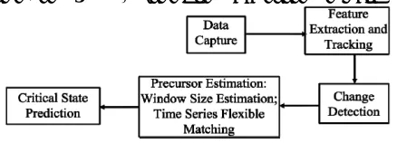
[image:14.595.62.281.148.227.2]A novel architecture and methodology for predicting critical states for complex physical systems is proposed here (see Figure 1). The conceptual architecture, main
Figure 1. An IIM Framework for Predicting Critical States in Complex Physical Systems.
processing stages, and flow of control are built around novel methods for modeling and prediction using statis-tical learning, in general, and semi-supervised learning and transduction, in particular. The architecture proposed approaches complex physical systems as a time evolving system; it parses and translates data streams into knowl-edge regarding the emergence of critical states. Towards that end, the specific methodology proposed here takes advantage of better sensor technology to employ ad-vanced computational methods for both data representa-tion and predicrepresenta-tion of critical states. While the method-ology proposed to map data into knowledge is generic, we apply the methods for predicting the genesis and in-tensification of cyclones.
The main processing stages are as follows:
1) Data capture: Archived Data and Near Real-Time (NRT) data are available for weather forecasting and modeling. Archived data are used for system training and validation, while NRT data are used for testing and op-erational purpose. These data are the inputs to the
proc-essing pipeline outlined in Figure. 1. To ensure rapid
data availability, the technique for NRT satellite data processing is different from science data product proc-essing. While NRT satellite data and related science products are not identical, the NRT data should be accu-rate enough for operational use. The data needed for pre-dicting cyclones are available from various NASA data archives.
2) Feature extraction and tracking: It produces the necessary high-dimensional feature vector and its time variation in order to find the change in the state of the physical system of interest. The feature extraction ap-proach is either an image data processing apap-proach or a dimensionality reduction approach, or a combination of both. Based on domain knowledge and predictive power, one decides on the features to use. Tracking and moni-toring of physical systems can be achieved using a Kal-man Filter approach or a particle filter approach. These
approaches have been shown to work robustly for tropi-cal cyclone tracking using multiple satellite observations [56,60].
3) Change detection using martingale: See Section 12. 4) Precursor estimation: The input from the change detection stage provides the temporal extent of signifi-cant events with only some of them preceding critical states. The events referred to as precursors are subject to classification using time-series flexible matching. The two step process is discussed next.
a) Window size estimation: The online martingale change detection approach is used to identify a data sub-sequence (time series) that behaves anomalously. First, two threshold values, θL and θR, are selected such that θL
< θR. As the system is monitoring the data (vector)
time-series sequence t (k), k = 1, 2, , martingale
val-ues M(i) at time instance i = 1, 2, , are computed.
When the first M (i) > θLis detected, one seeks for the
next time instance j when M (j) > θR. The window size
for this time series is j – i + 1, and the time series “win-dow” t = [t (i), t (i + 1), , t (j)] is extracted and re-corded as [T1, T2]. Note that the window is merely a
can-didate to serve as a PRECURSOR for a future critical
state. Hence, the θL and θR values are empirically
se-lected using Doob’s inequality [39] at a lower value, maybe less than 10, e.g. θL= 3 and θR= 4, which yields a
FAR of 25% to 33 1/3% (considered high). θL< θR
en-sures that a change is more likely to take place at the more recent time instance T2. This leads to a collection of
training sets where the sets differ by how far in time T2 is
away from the true critical state. As long as the martin-gale at (T2 + n) is greater than θL, the window [T1, T2] is
widen to [T1, T2 + n] to augment the set of potential
pre-cursors. The same process iterates until the martingale M (T2 + n) becomes less than θL. The next candidate
win-dow starts when the martingale M is again greater than θL.
The candidate precursors are subject to time-series flexi-ble matching to yield the similarity scores required for predicting critical states.
b) Time-series flexible matching and classification: In the time series classification problem, one assigns a label to an unlabeled time series based on training examples. The main research task for this problem involves similar-ity measures. Many similarsimilar-ity measures for data se-quences have been proposed [57]. The two main
catego-ries of similarity measures are the Lp-norm based
simi-larity measures and the elastic simisimi-larity measures. The Lp similarity measures are metric, but they assume fixed
length data sequences and do not support local time shifting; the elastic similarity can be used to compare arbitrary length data sequences and support local time shifting but they are not metric. The classical elastic
measure to overcome the weakness of Lp norms is the