Finite Elements Approaches in the Solution of Field Functions in Multidimensional Space: A Case of Boundary Value Problems

929

Finite Elements Approaches in the Solution of Field Functions in

Multidimensional Space: A Case of Boundary Value Problems

Chukwutoo Christopher Ihueze*1, Okafor Emeka Christian1, Edelugo Sylvester Onyemaechi2

1_{Department of Industrial ⁄ Production Engineering, Nnamdi Azikiwe University Awka.} 2_{Department of Mechanical Engineering University of Nigeria}

*Corresponding Author: ihuezechukwutoo @yahoo.com

ABSTRACT

An idealized two dimensional continuum region of GRP composite was used to develop an efficient method for solving continuum problems formulated for space domains. The continuum problem is solved by minimization of a functional formulated through a finite element procedure employing triangular elements and assumption of linear approximation polynomial. The assemblage of elements functional derivatives system of equations through FEM assembly procedure made possible the definition of a unique and parametrically defined model from which the solution of continuum configuration with an arbitrary number of scales is solved. The finite element method(FEM )developed is recommended to be applied in the evaluation of the function of functions in irregular shaped continuum whose boundary conditions are specified such as in the evaluation of displacement in structures and solid mechanics problems, evaluation of temperature distribution in heat conduction problems, evaluation of displacement potential in acoustic fluids evaluation of pressure in potential flows, evaluation of velocity in general flows, evaluation of electric potential in electrostatics, evaluation of magnetic potential in magnetostatics and in the solution of time dependent field problems. A unified computational model with standard error of 0.15 and correlation coefficient of 0.72 was developed to aid analysis and easy prediction of regional function with which the continuum function was successfully modeled and optimized through gradient search and Lagrange multipliers approach. Above all the optimization schemes of gradient search and Lagrangian multiplier confirmed local minimum of function as 0.006-0.00847 to confirm the predictions of FEM and constraint conditions.

1. INTRODUCTION

In calculus of variations, instead of attempting to locate points that extremize function of one or more variables that extremize quantities called functional, functions of functions that extremize the functional are found [1]. Also in the finite element process an approximate solution is sought to the problem of minimizing a functional. The concept of the finite element approach to elasticity as a process in which the total potential energy is minimized with respect to nodal displacements can obviously be extended to a variety of physical problems in which an extremum principle exists. The two concepts are combined in this study. Zienkiewicz and Cheung [2] applied similar approach to solve continuum problem expressed in derivative format employing the concept of functional minimization with FEM.

Above all, there are many problems encountered in engineering and physics where the minimization of the integrated quantity usually referred as functional and subject to some boundary conditions results in the exact solution.This functional may represent a physical recognizable variable in some instances, for many purposes it is simply a mathematically defined entity.

The geometry of field quantities or continuum may be a problem to close form solution of field functions encountered in engineering and science that appropriate algorithm becomes necessary to obtain optimum solution, it is then necessary to employ calculus of variation principles and FEM to obtain optimum continuum field functions whose boundary conditions are specified. The engineering field continuum problems can be basically in form of wave phenomenon, diffusion phenomenon and potential phenomenon usually represented by hyperbolic, parabolic and elliptic differential equations respectively [3].

The objective of this study is therefore to present a methodical approach to solve multiple dimensional field problems using integrated variational and FEM approach to establish relations for all elements functional of continuum where the minimization of the elements functionals system and solution are expected to give the stationary values of the function which extremize the functional.

2. THEORETICAL BACKGROUND

A finite element model of a two dimensional quadratic function is expected to present a methodical approach to employ for solution of multidimensional field functions that may have regular or irregular field regions. Zienkiewicz and Cheung [2] presented Euler theorem to approximate field functions if the integral or functional of the form

.

is to be minimized. The necessary and sufficient condition for this minimum to be reached is that the unknown function u (x, y, z) should satisfy the following differential equation

∂ ∂x [

∂f

∂(∂u/∂x) ] + ∂ ∂y [

∂f

∂(∂u/∂y) ] + ∂ ∂z [

∂f

∂(∂u/∂z) ] - ∂f

∂u = 0 (2)

within the same region, provided u satisfies the same boundary conditions in both cases,while the equation governing the behaviour of unknown physical quantity u can generally be expressed as

∂

∂x (kx∂_∂u_{x ) + ∂}∂_{y (k}y_∂∂u_{y ) + ∂}∂_z ( kz∂_∂u_{z ) + Q = 0} (3)

where

u = unknown function assumed to be single valued within the region kx, ky, kz , Q = specified functions of x, y, z

x, y, z = space variables

The equivalent formulation to that of equation (3) is the requirement that the volume integral given below and taken over the whole region, should be

χ =

∫∫∫

{1_{2 [k}x (∂_∂u_{x )} 2 + ky(∂_∂u_{y )}2 + kz(∂_∂u_{z )}2] - Q u}dxdydz (4)

subject to u obeying the same boundary conditions.

For two dimensional differential equation representing some physical quantities then

χ =

∫∫

{1_{2 [k}x (∂_∂u_{x )} 2 + ky(∂_∂u_{y )}2] - Q u}dxdy (5)

For the case of our interest, the equivalent functional to be minimized for 2-D Laplace model reduces to

χ =

∫∫

{1_{2 [k}x (∂_{∂x )}u 2 + ky(∂_∂u_{y )}2] }dxdy (6)

3. FINITE ELEMENT METHOD (FEM)

Euler variational minimum integral theorem was applied with the procedure of [4] on the general equation governing the behavior of field functions presented by [2] to develop a finite element version of elements functions functionals. The elements function functionals are minimized with respect to degrees of freedoms in the finite element method of assembly are applied to obtain the system model that is solved for the field of function . Basic approaches to achieve finite element solouttion of continuum are also available in [5-8}.

3.1 Formulation of Finite Elements Equations

The elements functional of the study are derived for each element and minimized using equation (6). Minimization of element functional entails finding the partial derivatives of the element functional at its nodes. The contributions of each element nodes are established and added for all continuum nodes to obtain the finite element model of the system. The formulation of finite element model starts by choosing the element type and then choosing the approximation polynomial coefficients are determined for establishing the element equations from where the interpolation functions for u are established for all elements. This function u is used then employed in finding the finite element model of the elements functionals from where the sought functions are found.

3.1.1 Discritization and element topology description

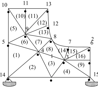
The region is discretized into 16 triangular elements with 26 degrees of freedom and assuming displacement in the global system of coordinate (horizontal direction only) only as in Figure 1 elements topologies are described in Table 1 for the establishment of element interpolation functions for the functional equations for the finite element minimization scheme.

[image:4.612.116.321.495.677.2]

Figure 1: Idealized Finite element Model of two Dimensional Composite Body.

.

.

.

.

.

.

.

.

.

.

.

.

.

.

.

(1)

(2) (3)

(4) (9) (6) (7)

(8) (14)(15) (16) (13)

(12) (11) (10)

(5)

10 11 13

5

14 15

3

6 7

8 12

4 9

1

[image:5.612.101.427.508.616.2]

Table 1: Element Topology Description.

Element Number

Active degrees of freedom of elements

Element coordinates Element nodes 1 u5, u4, u14, v5, v4, v14 (0,0), (0,21), (16,16) 14, 5, 4 2 u1, u4, u14, v1, v4, v14 (0,0), (16,16), (21, 0) 14, 4, 1 3 u1, u4, u3, v1, v4, v3 (21, 0), (16, 16), (25, 10) 1, 4, 3 4 u1, u3, u15, v1, v3, v15 (21, 0), (21, 0), (25, 10) 1, 3, 15 5 u5, u10, u9, v5, v10, v9 (0, 21), (0, 37), (10, 25) 5, 10, 9 6 u5, u9, u4, v5, v9, v4 (0, 21), (0, 25), (16, 16) 5, 9, 4 7 u9, u4, u8, v9, v4, v8 (16, 16), (10, 25), (22, 13) 4, 9, 8 8 u8, u4, u3, v8, v4, v3 (16, 16), (22, 23), (25, 10) 4, 8, 3 9 u15, u3, u2, v15, v3, v2 (25, 10), (35, 10), (35, 0) 15, 3, 2 10 u9, u10, u11, v9, v10, v11 (0, 37), (10, 37), (10, 25) 9, 10, 11 11 u9, u11, u13, v9, v11, v13 (10, 25), (10, 37), (18, 37) 9, 11, 13 12 u9, u13, u12, v9, v13, v12 (10, 25), (18, 37), (19, 29) 9, 13, 12 13 u9, u12, u8, v9, v12, v8 (10, 25), (19, 29), (22, 23) 9, 12, 8 14 u3, u8, u7, v3, v8, v7 (25, 10), (22, 23), (29, 19) 3, 8, 7 15 u3, u7, u6, v3, v7, v6 (25, 11), (29, 19), (35, 18) 3, 7, 6 16 u3, u6, u12, v3, v6, v12 (25, 10), (35, 18), (35, 10) 3, 6, 2

3.2Determination of FEM Characteristics

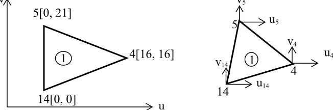
3.2.1 Element 1 interpolation and functional equation formulation

By assuming a linear approximation polynomial of the form

y

a

x

a

a

y

x

u

(

,

)



₀



₁



₂ (1)

and following the method of Ihueze etal (2009) and Asterly (1992) 5[0, 21]

4[16, 16]

14[0, 0] 1

u v

u4

v5

1 5

v14

u14

v4

u5

Where a0, a1, a2 are called polynomial coefficients or shape constants so that by passing (1) through the nodes of element1the system of unknown function of the element becomes:

14 2 14

1 0

14

a

a

x

a

y

u







4 2 4

1 0

4

a

a

x

a

y

u







5 2 5

1 0

5

a

a

x

a

y

u







Putting the above polynomial function in matrix form then                                5 4 14 2 1 0 5 5 4 4 14 14 1 1 1 u u u a a a y x y x y x

By applying Crammers rule















14 4 5 5 4 4 5 14 14 5 5 14 4 4 14



21

0 u x y x y u x y x y u x y x y

a  _A     

(2)







14 4 5 4



5 14



5



14 4



21

1 u y y u y y u y y

a  _A     







14 5 4 4



14 5



5



4 14



21

2 u x x u x x u x x

a  _A     

Substituting (2) in (1) then

y a x a a

u₁  ₀  ₁  ₂





































u x x u



x x



u



x x



y x y y u y y u y y u y x y x u y x y x u y x y x u u A A A 14 4 5 5 14 4 4 5 14 21 4 14 5 14 5 4 5 4 14 2 1 14 4 4 14 5 5 14 14 5 4 4 5 5 4 14 21 1                   (3)

Recall that the approximation function is given as

5 5 4 4 14

14u N u N u

N

u    (4)

 

x

y





x

y

x

y

 

y

y

 

x

x

x





y

N

₁₄

,



₂1_{A 4 5}



_{5 4}



₄



₅



₅



₄ (5)

 

x

y





x

y

x

y





y

y

 

x

x

x



y

N

₄

,



₂1_{A 5 14}



_{14 5}



₅



₁₄



₁₄



₅

 

x

y





x

y

x

y





y

y

 

x

x

x



y

N

₅

,



₂1_{A 14 4}



_{4 14}



₁₄



₄



₄



₁₄

But A = 12





x4y5 x5y4

 

 x5y14x14y5

 

 x14y4 x4y14





_{= 168mm}2 ₍₆₎

where A= area of triangular element so that



x y



N ₁₄  ₃₃₆1 336  5  16



x



N 4  ₃₃₆1 21



x y



N 5  ₃₃₆1  16 16

Substituting (7) in (4)





14 3361





4 3361





5

3361 336 5x 16y u 21x u 16x 16y u

u       

336 16 336 21 336

5u₁₄ u₄ u₅ x

u _  _{ } 



336 16 336

16u₁₄ u₅ y

u _  _

 

By assuming a two dimensional Laplace function for the continuum function of the form

∂2u ∂x2 +

∂2u

∂y2 = 0 (10)

The minimum function integral called functional to be minimized becomes in which case

kx = ky = kz = 1 and Q = 0 (11)

So that (4 ) reduces to

 

 







_





_





_





_dxdy

x

u_y

x

u 2 2

2

1

(9) (8)

By substitutingg the first partial derivatives of the element 4 interpolation functions in ( 12) with

dxdy = A = 168

2 5 2 4 5 4 14 5 14 4 2

14 0.313 0.524 _0.656 0.762

418 .

0 u u u u u u u u u

x     

(13)

By differentiating w.r.t.u14,u4,and u5



0.836 ₁₄ 0.313 ₄ 0.524 ₅



*0.5

14

u u

u u

x _{  }

 



1.312 ₄ 0.313 _{14 5}



*0.5

4

u u u

u

x _{  }

 



1.524 ₅ 0.524 _{14 4}



*0.5

5

u u u

u

x _{  }

 

3.2.2 Element 2 interpolation and functional equation formulation

By assuming a linear approximation polynomial of the form

y a x a a y x

u ( _, )  ₀  ₁  ₂ (15)

Passing (15) through the nodes then

14 2 14

1 0

14 a a x a y

u   

1 2 1

1 0

1 a a x a y

u   

4 2 4

1 0

4 a a x a y

u   

Putting the system in matrix form then

By applying Crammers rule,















14 1 4 4 1 14 1 4 14 4 1



21

0 u x y x y u y y u x x

a  _A     







1 4 14 14 4 1



4 14



1



14 4

 

2 1

1 u x y x y u y y u x x

a  _A     







4 14 1 1 14 4



14



4



1 14



2 1

2 u x y x y u y y u x x

a  _A      (16)

Substituting (16) in (15)

































₂1

_u

₁₄

_x

₁

_y

₄

_x

₄

_y

₁

_u

₁₄

_y

₁

_y

₄

_u

₁₄

_x

₄

_x

₁

u

_A







u

₁

x

₄

y

₁₄



x

₁₄

y

₄



u

₁



y

₄



y

₁₄





u

₁



x

₁₄



x

₄





(17)







u

4

x

14

y

1



x

1

y

14



u

4



y

14



y

1





u

4



x

1



x

14





Recalling that the approximation function is

4 4 1 1 14

14u N u N u

N

u    (18)

Comparing (18) and (17) then



 

 





x y x y y y x x x



y

N₁₄  ₂1_{A 1 4}  _{4 1}  ₁  ₄  ₄  ₁







x y x y



y y

 

x x x



y

N1  21_A 4 14  14 4  4  14  14  4







x y x y



y y

 

x x x



y

N₄  ₂1_{A 14 1}  _{1 14}  ₁₄  ₁  ₁  ₁₄ (19)

But A = 12





x1y4  x4y1

 

 x4y14  x14y4

 

 x14y1 x1y14





_=168mm2 ₍₂₀₎

so that















x x y

N₁₄  ₃₃₆1 336  0 16  16  21  ₃₃₆1 336 16  5

 



x



 

y



x y



N₁  ₃₃₆1 0 16  0  016  ₃₃₆1 16 16

   

 

y



y



N4  ₃₃₆1 0 0  21  0  ₃₃₆1 21 (21)

Substituting (22) into (18)





14 3361





1 3361





4

3361 336 16x 5y u 16 16y u 21y u

u      

21 21

336 16 336

16u₁₄ u₁ u₁₄ u₁ x

u _  _{ }  _   16 21 336 5 336 21 336 16 336

5u₁₄ u₁ u₁₄ u₁₄ u₁ u₄

y

u _  _{  }  _{ }

 

(23)

By substitutingg the first partial derivatives of the element 4 interpolarion functions in ( 12) with dxdy = A = 168mm2



2



4 4 1 14 4 2 1 14 1 2

14 0.3611 0.38 0.156 0.5 0.328

190 .

0 u u u u u u u u u

x       ₍₂₄₎

By differentiating w.r.t.u14,u1,and u4

4 1 14 14 156 . 0 261 . 0 418 .

0 u u u

u x      5 14 1 1 5 . 0 261 . 0 76 .

0 u u u

u x      1 14 4 4 5 . 0 156 . 0 656 .

1 u u u

u

x _{  }

 

(25)

3.2.3 Element 3 interpolation and functional equation formulation

By assuming a linear approximation polynomial of the form



x y



a a x a y

u ,  ₀  ₁  ₂ (26)

and passing (26) through the nodes then

1 2 1

1 0

1 a a x a y

u   

3 2 3

1 0

3 a a x a y

u   

4 2 4

1 0

4 a a x a y

u   

v

[16, 16] 4

3 [25, 10]

Putting the above equations in matrix form then,

  

 

  

     

 

  

 

  

 

  

 

4 3 1

2 1 0

4 4

3 3

1 1

1 1 1

u u u

a a a

y x

y x

y x

(27)

By applying Crammers rule,















1 3 4 4 3 1 3 4 1 4 3



21

0 u x y x y u y y u x x

a  _A     







3 4 1 1 4 3



4 1



3



1 4



21

1 u x y x y u y y u x x

a  _A     







4 1 3 3 1 4



1 3



4



3 1



21

2 u x y x y u y y u x x

a  _A     

(28) Substituting (28) into (26)

































₂1

_u

₁

_x

₃

_y

₄

_x

₄

_y

₃

_u

₁

_y

₃

_y

₄

_u

₁

_x

₄

_x

₃

u

_A







u

₃

x

₄

y

₁



x

₁

y

₄



u

₃



y

₄



y

₁





u

₃



x

₁



x

₄











u

₄

x

₁

y

₃



x

₃

y

₁



u

₁



y

₁



y

₃





u

₄



x

₃



x

₁





(29)

Recall that the approximation function or interpolation function is expressed as:

4 4 3

3 1

1u N u N u

N

u    (30)

Comparing (29) and (30) then,



 

 





x y x y y y x x x



y

N₁  ₂1_{A 3 4}  _{4 3}  ₃  ₄  ₄  ₃







x y x y



y y

 

x x x



y

N₃  ₂1_{A 4 1}  _{1 4}  ₄  ₁  ₁  ₄







x y x y



y y

 

x x x



y

N₄  ₂1_{A 1 3}  _{3 1}  ₁  ₃  ₃  ₁

(31)

But A = 1₂





_{x1y4  x4y3}

 

_{ x4y1 x1y4}

 

_{ x1y3  x3y1}





= 57mm2 ₍₃₂₎

then



 

 

x



y



x y



N₁ ₁₁₄1 400160  1016  1625 ₁₁₄1 2406 9



 

 

x



y



x y



N₃ ₁₁₄1 0336  160  2116 ₁₁₄1 33616 5



 

 

x



y



x y



N₄ ₁₁₄1 5250  010  2521 ₁₁₄1 52510 4

Substituting (30) into (31)





1 1141





3 1141





4

1141 240 6x 9y u 336 16x 5y u 525 10x 4yu

u         

114 10 114

16 114

6u1 u3 u₁₄

x

u _  _{ } 

  114 4 114 5 114

9u₁ u₃ u₄ y

u _  _{ }

 

(34)

By substitutingg the first partial derivatives of the element 4 interpolarion functions in ( 12) with dxdy = A = 57

2 4 4 3 2 3 4 1 3 1 2

1 0.224 0.105 0.616 0.789 0.254

257 .

0 u uu uu u uu u

x      ₍₃₅₎

By differentiating w.r.t.u1,u3, and u4

4 3 1 1 105 . 0 224 . 0 514 .

0 u u u

u x      4 1 3 3 789 . 0 224 . 0 232 .

0 u u u

u

x _{  }

  3 1 4 4 789 . 0 105 . 0 508 .

1 u u u

u

x _{  }

 

(36)

3.2.4 Element 4 interpolation and functional equation formulation

By substitutingg the first partial derivatives of the element 4 interpolarion function in (12)

2 3 15 3 3 1 2 15 15 1 2

1 0.214 0.207 0.5 0.2 0.35

357 .

0 u uu u uu uu u

x     

(37) By differentiating w.r.t.u1,u15, and u3

3 15 1 1 5 . 0 2144 . 0 714 .

0 u u u

du dx    3 1 15 15 2 . 0 214 . 0 414 .

0 u u u

du

dx _{  }

15 1 3 3 2 . 0 5 . 0 7 .

0 u u u

du

dx _{  }

3.2.5 Element 5 interpolation and functional equation formulation

By substitutingg the first partial derivatives of the element 4 interpolarion functions in (12) with dxdy = A =57mm2

2 10 10 9 2 9 10 5 9 5 2

5 0.6 0.163 0.4 0.2 0.181

35 .

0 u uu uu u uu u

x      ₍₃₉₎

By differentiating w.r.t.u5,u9,and u10

10 9 5 5 163 . 0 6 . 0 70 .

0 u u u

u x      10 5 9 9 2 . 0 6 . 0 80 .

0 u u u

u x      9 5 10 10 2 . 0 163 . 0 362 .

0 u u u

u x      (40)

3.2.6 Element 6 interpolation and functional equation formulation By similar procedures as above,

2 5 9 5 2 9 9 4 5 4 2

4 0.105 0.614 0.616 0.618 0.257

254 .

0 u u u uu u u u u

x     

(41) By differentiating w.r.t.u4,u9,and u5

10 9 5 4 508 .

0 u u u

u x      5 5 9 9 618 . 0 614 . 0 232 .

1 u u u

u x      9 4 5 5 618 . 0 105 . 0 514 .

0 u u u

u

x _{  }

 

(42)

3.2.7 Element 7 interpolation and functional equation formulation By similar procedures as above,

2 9 9 8 2 8 9 4 8 4 2

4 0.469 0.302 0.305 0.141 0.221

385 .

0 u u u u u u u u u

x     

9 8 4 4 302 . 0 469 . 0 77 .

0 u u u

u x      9 4 8 8 141 . 0 469 . 0 61 .

1 u u u

u

x _{  }

  9 4 9 9 141 . 0 302 . 0 442 .

0 u u u

u

x _{  }

 

(44)

3.2.8 Element 8 interpolation and functional equation formulation By similar procedures as above,

2 4 8 4 2 8 4 3 8 3 2

3 0.61 0.369 0.295 0.530 0.450

215 .

0 u uu uu u u u u

x     

(45) By differentiating w.r.t.u3,u8,and u4

4 8 3 3 369 . 0 061 . 0 430 .

0 u u u

u x      4 3 8 8 530 . 0 061 . 0 590 .

0 u u u

u x      9 3 4 4 530 . 0 369 . 0 90 .

0 u u u

u x      (46)

3.2.9 Element 9 interpolation and functional equation formulation By similar procedures as above,

15 2 2 15 2 3 3 2 2

2 0.5 0.25 0.25 0.5

5 .

0 u uu u u uu

x    

(47) By differentiating w.r.t.u2,u3,and u15

15 3 2 2 5 . 0 5 .

0 u u

u u x      2 3 3 5 . 0 5 .

0 u u

u x     2 15 15 5 . 0 5 .

0 u u

u

x _{ }

 

(48)

11 9 2 9 2 10 11 10 2

11 0.61 0.3 0.208 0.417

508 .

0 u u u u u uu

x    

(49) By differentiating w.r.t.u11,u10, and u9

9 10 11 11 417 . 0 6 . 0 016 .

1 u u u

u

x _{  }

  11 10 10 6 . 0 6 .

0 u u

u

x _{ }

  11 9 9 417 . 0 416 .

0 u u

u

x _{ }

 

(50)

3.2.11 Element 11 interpolation and functional equation formulation By similar procedures as above,

11 9 2 9 2 11 13 11 2

13 0.75 0.542 0.167 0.333

375 .

0 u u u u u uu

x    

(51) By differentiating w.r.t.u9,u13, and u1

11 9 9 333 . 0 334 .

0 u u

u x     11 13 13 75 . 0 75 .

0 u u

u x     9 13 11 11 333 . 0 75 . 0 084 .

1 u u u

u x      (52)

3.2.12 Element 12 interpolation and functional equation formulation By similar procedures as above,

2 13 13 12 2 12 13 9 12 9 2

9 0.68 0.151 0.68 0.158 0.319

214 .

0 u u u uu u u u u

x     

By differentiating w.r.t.u9,u12, and u13

13 12 9 9 151 . 0 684 . 0 428 .

0 u u u

u

x _{  }

  3 9 12 12 158 . 0 684 . 0 368 .

1 u u u

u

x _{  }

  12 9 13 13 158 . 0 151 . 0 638 .

0 u u u

u

x _{  }

 

3.2.13 Element 13 interpolation and functional equation formulation By similar procedures as above,

2 9 12 9 2 12 9 8 12 8 2

8 0.758 0.386 0.561 0.182 0.170

367 .

0 u u u u u u u u u

x     

(54) By differentiating w.r.t.u8, u12, and u9

9 12 8 8 386 . 0 758 . 0 734 .

0 u u u

u

x _{  }

  9 8 12 12 182 . 0 758 . 0 122 .

1 u u u

u

x _{  }

  12 8 9 9 182 . 0 386 . 0 34 .

0 u u u

u

x _{  }

 

(55)

3.2.14 Element 14 interpolation and functional equation formulation By similar procedures as above,

2 8 8 7 2 7 8 3 7 3 2

3 0.462 0.051 0.563 0.665 0.307

206 .

0 u uu uu u uu u

x     

(56) By differentiating w.r.t.u3,u7, and u8

8 7 3 3 051 . 0 462 . 0 412 .

0 u u u

u x      8 3 7 7 665 . 0 462 . 0 126 .

1 u u u

u x      7 3 8 8 665 . 0 51 . 0 614 .

0 u u u

u x      (57)

3.2.15 Element 15 interpolation and functional equation formulation By similar procedures as above,

2 7 7 6 2 6 7 3 6 3 2

3 0.154 0.51 0.385 0.923 0.716

178 .

0 u uu uu u uu u

x     

7 6 3 3 51 . 0 154 . 0 356 .

0 u u u

u x      7 6 3 3 51 . 0 154 . 0 356 .

0 u u u

u

x _{  }

  6 3 7 7 923 . 0 51 . 0 432 .

1 u u u

u

x _{  }

 

(58)

3.2.16 Element 16 interpolation and functional equation formulation By similar procedures as above,

2 6 6 2 2 2 3 2 2

3 0.4 0.513 0.625 0.313

2 .

0 u u u u u u u

x    

By differentiating w.r.t.u3, u2 and u6

2 3 3 4 . 0 4 .

0 u u

u x     6 3 2 2 625 . 0 4 . 0 026 .

0 u u u

u

x _{  }

  2 6 6 625 . 0 626 .

0 u u

u

x _{ }

 

(59)

4. SYSTEM ELEMENTS ASSEMBLY ALGORITHMS

The algorithms for element assembly involves the addition of all elements contributing to

minimization dX

e

du , this leads to system of equations that equals the degrees of freedoms in the

continuum, the derivatives are then added in a special format called assembly. There are 15 effective degrees of freedoms for the assembly of 16 elements

dX_ e

ui = 0, i = 1, 2, 3,……, 16

For

i = 1, X

e

u1 = 0 (60)

i = 2, X

e

u2

i = 3, X

e

u3 = 0 (62)

i = 4, X

e

u4 = 0 (63)

i = 5, X

e

u5 = 0 (64)

i = 6, X

e

u6 = 0 (65)

i = 7, X

e

u7 = 0 (66)

i = 8, X

e

u8 = 0 (67)

i = 9, X

e

u9 = 0 (68)

i = 10, X

e

u10

= 0 (69)

i = 11, X

e

u11

= 0 (70)

i = 12, X

e

u12 = 0 (71)

i = 13, X

e

u13 = 0 (72)

i = 14, X

e

u14 = 0 (73)

i = 15, X

e

u15 = 0 (74)

5. ELEMENTS EQUATIONS ASSEMBLY

All the partial derivatives resulting from the minimization scheme with respect to the fifteen (15) active degrees of freedom (DOF) are added as follows the superscripts on these equations denote element sources:

X

u1

= _Xe

u1

= 0 = X

2

u1

+ X

3

u1

+ X

4

u1

= 1.988u1 – 0.724u3 - 0.105u4 – 0.5u5 – 0.261u14 – 0.214u15 (75)

X

u2 = 

Xe

u2 = 0 =

X9

u2 +

X16

u2

X

u3 = 

Xe

u3 = 0 =

X16

u3 +

X15

u3 +

X14

u3 +

X9

u3 +

X4

u3 +

X3

u3 +

X8

u3

= - 0.724u1 – 0.9u2 + 3.03u3 – 1.158u4 + 0.154u6 – 0.972u7 – 0.001u8 - 0.2u15 (77)

X

u4

= _Xe

u4

= 0 = X

1

u4

+ X

2

u4

+ X

3

u4

+ X

6

u4

+ X

7

u4

+ X

8

u4

= -1.158u3 + 5.49u4 – 0.395u1 + 0.008u5 – 0.469u8 – 1.832u9 – u10 – 0.001u14 (78)

X

u5 = 

Xe

u5 = 0 =

X1

u5 +

X5

u5 +

X6

u5

= - 0.409u4 + 1.979u5 – 1.218u9 – 0.163u10 – 0.262u14 (79)

X

u6

= _Xe

u6

= 0 = X

15

u6

+ X

16

u6

= 1.396u6 – 0.625u2 + 0.154u3 – 0.923u7 (80)

X

u7 = 

Xe

u7 = 0 =

X15

u7 +

X14

u7

= 2.549u7 – 0.972u3 – 0.923u6 – 0.665u9 (81)

X

u8

= _Xe

u8

= 0 = X

7

u8

+ X

8

u8

+ X

13

u8

+ X

14

u8

= 0.449u3 – 0.999u4 – 0.665u7 + 3.548u8 + 0.245u9 – 0.758u12 (82)

X

u9 = 

Xe

u9 = 0 =

X13

u9 +

X12

u9 +

X11

u9 +

X10

u9 +

X7

u9 +

X6

u9 +

X5

u9

= - 0.302u4 – 1.832u5 + 0.386u8 + 3.851u9 – 0.20u10 – 0.75u11 + 0.502u12 + 0.151u13 (83)

X

u10

= _Xe

u10

= 0 = X

5

u10

+ X

10

u10

= - 0.163u5 – 0.2u9 + 0.962u10 – 0.6u11 (84)

X

u11 = 

Xe

u11 = 0 =

X11

u11 +

X10

u11

= - 0.75u9 – 0.6u10 + 2.1u11 - 0.75u13 (85)

X

u12

= _Xe

u12

= 0 = X

13

u12

+ X

12

u12

X

u13 = 

Xe

u13 = 0 =

X11

u13 +

X12

u13

= - 0.151u9 – 0.75u11 – 0.158u12 + 1.388u13 (87)

X

u14

= _Xe

u14

= 0 = X

2

u14

+ X

1

u14

= - 0.261u1 – 0.313u4 – 0.262u5 + 0.836u14 (88)

X

u15 = 

Xe

u15 = 0 =

X4

u15 +

X9

u15

= - 0.214u1 – 0.5u2 – 0.2u3 + 0.914u15 (89)

6. APPLICATION OF BOUNDARY CONDITION

In this work a special case where displacements at the boundaries are limited to 0.5mm for an irregular continuum is considered to predict continuum displacement, strain and stress functions, while the constrained conditions are taken as zero so that by equating u14 = u15 = 0 and u2 = u5= u6 = u8 = u10= u13 = 0.50 , (75 - 89) transform to the following:

1.988u1 – 0.724u3 – 0.105u4 = 0.25 (90)

0.900u3 = 0.201 (91)

- 0.724u1 + 3.03u3 – 0.158u4 – 0.972u7 = 0.374 (92)

- 1.158u3 + 5.490u4 – 0.395u1 = 0.731 (93)

- 0.409u4 – 1.218u9 = - 0.907 (94)

0.154u3 – 0.923u7 = - 0.386 (95)

2.549u7 – 0.972u3 – 0.665u9 = 0.462 (96)

0.449u3 – 0.999u4 – 0.665u7 + 0.245u9 – 0.758u12 = - 1.774 (97)

3.851u9 – 0.302u4 – 0.75u11 + 0.502u12 = 0.748 (98)

2.100u11 – 0.750u9 = 0.675 (100)

- 0.153u3 + 0.502u9 + 2.490u12 = - 0.379 (101)

- 0.151u9 – 0.750u11 – 0.158u12 = - 0.694 (102)

- 0.261u1 – 0.313u4 = 0.131 (103)

- 0.214u1 – 0.200u3 = 0.250 (104)

7. SOLUTION AND POST PROCESSING FOR CONTINUUM FUNCTION

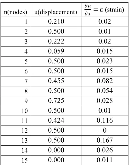
[image:21.612.199.413.433.706.2]

The following nodal displacements in mm are further evaluated by first evaluating u3 = 0.222 from (91) so that other nodal values of the displacement function is as presented in Table 2. The first partial derivatives of the interpolation function evaluated with active degree of freedom in of element with respect to the x axis gives the slope of the function and also gives the value of the strain as presented in Table 2. The computations are achieved with sixteen elements interpolation functions associated with the elements global coordinate axis. The strains so computed may be used with Hooke’s law of elasticity to predict the stress distribution function at the respective nodes when the elastic modulus is known from literature.

Table 2: FEM Results.

n(nodes) u(displacement)  (strain)

1 0.210 0.02

2 0.500 0.01

3 0.222 0.02

4 0.059 0.015

5 0.500 0.023

6 0.500 0.015

7 0.455 0.082

8 0.500 0.054

9 0.725 0.028

10 0.500 0.01

11 0.424 0.116

12 0.500 0

13 0.500 0.167

14 0.000 0.026

The stress prediction model of a material within the elastic limit is expressed as

σ = Е (105)

where Е = modulus of elasticity

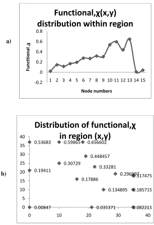
The excel graphics of FEM result using Table 2 of Figure 2 shows a serious indication that the minimum value of the function is between node 14 and 15 hence another extremization method is needed to point at which point of the region is this extremum.

Figure 2: Distribution of Function within the Region.

8. DISCUSSION AND VALIDATION OF RESULTS

Regression analysis was carried out on FEM results to obtain a unified model for elements function interpolation. The regression model so obtained is further used to transform the element functional equation to aid extremization of FEM results.

8.1 Regression Analysis

Multiple linear regression analysis was carried out on finite element results to obtain the

following model for the region. By employing the classical multiple linear regression equation of the form

u(x, y) = ao + a1 x+ a2y (106) ‐0.2

0 0.2 0.4 0.6 0.8

1 2 3 4 5 6 7 8 9 10 11 12 13 14 15

Function,u(x,y)

Nodal Points

Distribution

 

of

  

function,u(x,y)

 

within

 

a regression model for the FEM is obtained with Table 3 and expressed as (107).

u(x,y) = 0.065 + 0.0036x + 0.0130y (107)

The goodness of fit of regression was evaluated to obtain: Coefficient of determination, r2 = 0.52, correlation coefficient, r = 0.72, standard error, se = 0.1

where u = field function evaluated through FEM u1 = average of FEM function

up = field function predicted with regression model

Table 2 and Figure 2 show the variation of the function within the region. Continuum fluid elements in heat and mass transfer operations associated with pipeline transportation can elegantly be analyzed following the procedure of this work. The FEM developed can be applied in the evaluation of the stress distribution in irregular shaped continuum whose boundary conditions are specified such as in the evaluation of displacement in structures and solid mechanics problems, evaluation of temperature distribution in heat conduction problems, evaluation of displacement potential in acoustic fluids ,evaluation of pressure in potential flows ,evaluation of velocity in general flows, evaluation of electric potential in electrostatics and in evaluation of magnetic potential in magnetostatics.

8.2 Extremization of Functional: Extremization by Lagrange Multipliers Approach

In order to further analyse the FEM results, the functional, of any element is transformed to a function of (x, y) using the regression model of (107) to obtain:

χ f x, y 0.000042x 0.0017y 0.000059x 0.00034y 0.00015xy 0.00847 108

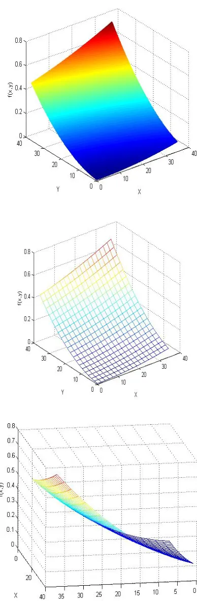
Figure 4a,b and c show versions of 3D plots of function using Matlab for (108) The objective function

f x, y 0.000042x 0.0017y 0.000059x 0.00034y 0.00015xy 0.00847

subject to the constraint relations

u x, y 0.5 0.0225x 0.5 109

u x, y 0.0201x 0.0238y 0 110

[image:24.612.70.548.132.666.2]

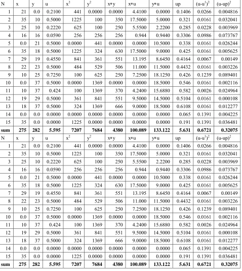
Table 3 Computations For Regression and Error Analysis of FEM Results.

N x y u x2 _y2 _{xy xu yu up (u-u}1₎2 _(u-up)2

1 21 0.0 0.2100 441 0.0000 0.0000 4.4100 0.0000 0.1406 0.0266 0.004816 2 35 10 0.5000 1225 100 350 17.5000 5.0000 0.321 0.0161 0.032041 3 25 10 0.2220 625 100 250 5.5500 2.2200 0.285 0.0228 0.003969 4 16 16 0.0590 256 256 256 0.944 0.9440 0.3306 0.0986 0.073767 5 0.0 21 0.5000 0.0000 441 0.0000 0.0000 10.5000 0.338 0.0161 0.026244 6 35 18 0.5000 1225 324 630 17.5000 9.0000 0.425 0.0161 0.005625 7 29 19 0.4550 841 361 551 13.195 8.6450 0.4164 0.0067 0.00149 8 22 23 0.5000 484 529 506 11.000 11.5000 0.4432 0.0161 0.003226 9 10 25 0.7250 100 625 250 7.2500 18.1250 0.426 0.1239 0.089401 10 0.0 37 0.5000 0.0000 1369 0.0000 0.0000 18.5000 0.546 0.0161 0.002116 11 10 37 0.424 100 1369 370 4.2400 15.6880 0.582 0.0026 0.024964 12 19 29 0.5000 361 841 551 9.5000 14.5000 0.5104 0.0161 0.000108 13 18 37 0.5000 324 1369 666 9.0000 18.5000 0.6108 0.0161 0.012277 14 0.0 0.0 0.0000 0.0000 0.0000 0.0000 0.0000 0.0000 0.065 0.1391 0.004225 15 35 0.0 0.0000 1225 0.0000 0.0000 0.0000 0.0000 0.191 0.1391 0.036481

sum 275 282 5.595 7207 7684 4380 100.089 133.122 5.631 0.6721 0.32075

N x y u x2 _y2 _{xy xu yu up (u-u}1₎2 _(u-up)2

1 21 0.0 0.2100 441 0.0000 0.0000 4.4100 0.0000 0.1406 0.0266 0.004816 2 35 10 0.5000 1225 100 350 17.5000 5.0000 0.321 0.0161 0.032041 3 25 10 0.2220 625 100 250 5.5500 2.2200 0.285 0.0228 0.003969 4 16 16 0.0590 256 256 256 0.944 0.9440 0.3306 0.0986 0.073767 5 0.0 21 0.5000 0.0000 441 0.0000 0.0000 10.5000 0.338 0.0161 0.026244 6 35 18 0.5000 1225 324 630 17.5000 9.0000 0.425 0.0161 0.005625 7 29 19 0.4550 841 361 551 13.195 8.6450 0.4164 0.0067 0.00149 8 22 23 0.5000 484 529 506 11.000 11.5000 0.4432 0.0161 0.003226 9 10 25 0.7250 100 625 250 7.2500 18.1250 0.426 0.1239 0.089401 10 0.0 37 0.5000 0.0000 1369 0.0000 0.0000 18.5000 0.546 0.0161 0.002116 11 10 37 0.424 100 1369 370 4.2400 15.6880 0.582 0.0026 0.024964 12 19 29 0.5000 361 841 551 9.5000 14.5000 0.5104 0.0161 0.000108 13 18 37 0.5000 324 1369 666 9.0000 18.5000 0.6108 0.0161 0.012277 14 0.0 0.0 0.0000 0.0000 0.0000 0.0000 0.0000 0.0000 0.065 0.1391 0.004225 15 35 0.0 0.0000 1225 0.0000 0.0000 0.0000 0.0000 0.191 0.1391 0.036481

By taking partial derivatives of Lagrange expression

L x, y, λ ,λ f x, y λ g x, y λ g x, y 111

0.000042x 0.0017y 0.000059x 0.00034y 0.00015xy 0.00847

λ 0.0225x λ 0.0201x 0.0238y

to obtain the following relations

∂L

∂x 0.000042 0.0001x 0.00015y 0.0225λ 0.0201λ 0 112

∂L

∂y 0.0017 0.0068y 0.00015x 0.0225λ 0.0238λ 0 113

∂L

∂λ 0.0225x 0 114

∂L

∂λ 0.0201x 0.0238y 0 115

By solving (107)- (110) from(109)

0, λ 0.0356, λ 0.0378

By substituting the variables in (108) the optimum value of the function is obtained as

u(x,y) = f(x,y) = 0.00847

χ f x, y 0.000042x 0.0017y 0.000059x 0.00034y 0.00015xy 0.00847 108

The prediction of functional, χ with (108) are presented in Table 4 using excel package to draw conclusion with the FEM and multiple linear regression results of Table 3.

Table 4: Prediction of Functional with Equation (108).

N x Y Χ

1 21 0 0.035371

2 35 10 0.185715

3 25 10 0.134895

4 16 16 0.176886

5 0 21 0.19411

6 35 18 0.317475

7 29 19 0.296997

8 22 23 0.33281

9 10 25 0.30729

10 0 37 0.53683

11 10 37 0.59865

12 19 29 0.448457

13 18 37 0.656602

14 0 0 0.00847

15 35 0 0.082215

Tables 3 and 4 are compared for u , up and their functional, χ are found approximate.

8.2.1 Extremization by Lagrange gradient search approach

The extremum conditions for continuous and differentiable functions are defined [1] as follows:

f _{. . .} f _{. . .}

f . f .

Since fxx and fyy > 0  minimum extremum or local extremum exists.

8.2.2 Extremization by Lagrange multipliers approach By expressing (108) in the form

f x, y 0.000042x 0.0017y 0.000059x 0.00034y 0.00015xy 0.00847

Subject to the constraint relations

u x, y 0.5 0.0225x 0.5 120

u x, y 0.0201x 0.0238y 0 121   derived for nodes 14 and 10 of elements 1 and 5 at the boundaries.

By taking partial derivatives of Lagrange expression

L x, y, λ ,λ x, y λ g x, y λ g x, y 122

0.000042x 0.0017y 0.000059x 0.00034y 0.00015xy 0.00847  λ 0.0225x λ 0.0201x 0.0238y

to obtain the following relations

∂L

∂x 0.000042 0.0001x 0.00015y 0.0225λ 0.0201λ 0 123

∂L

∂y 0.0017 0.0068y 0.00015x 0.0225λ 0.0238λ 0 124

∂L

∂λ 0.0225x 0 125

∂L

∂λ 0.0201x 0.0238y 0 126

By solving (123)- (126) starting from(125)

0, λ 0.0356, λ 0.0378

[image:28.612.137.443.66.513.2]

Figure 3a, b Distribution of function within the Region.

‐0.2 0 0.2 0.4 0.6 0.8

1 2 3 4 5 6 7 8 9 10 11 12 13 14 15

Functtional

 

,

χ

Node numbers

Functional,

χ

(x,y)

 

distribution

 

within

 

region

0.035371

0.185715 0.134895

0.17886 0.19411

0.317475 0.296997 0.33281

0.30729 0.53683 0.59865

0.448457 0.656602

0.00847 0.082215

0 5 10 15 20 25 30 35 40

0 10 20 30 40

Distribution

 

of

 

functional,

χ

in

 

region

 

(x,y)

[image:29.612.205.399.80.670.2]

9. CONCLUSSIONS

The methods of this article apply to:

1. Solution of boundary value engineering phenomena whose function can be expressed as partial differential equation.

2. Solution of of displacement in structures and solid mechanics problems, temperature distribution in heat conduction problems, displacement potential in acoustic fluids , pressure in potential flows , velocity in general flows, electric potential in electrostatics magnetic potential in magnetostatics , torsion of non – homogenous shaft, flow through an anisotropic porous foundation, axi – symmetric heat flow, hydrodynamic pressures on moving surfaces

3. Solution of time dependent field problems such as creep, fracture and fatigue.

4. Equations (97) and (98) are recommended for the prediction of possible values of the displacement function of GRP composites region from where other properties of the region could be evaluated.

5. A unified computational model with standard error of 0.15 and correlation coefficient of 0.72 was developed to aid analysis and easy prediction of regional function with which the continuum function was successfully modeled and optimized through gradient search and Lagrange multipliers approach.

6. The MatLab 3-D graphics of Figure 4 show potential trend of function within the regionwith minimum and maximum at the boundaries.

REFERENCES

[1] Amazigo, J.C and Rubenfield, L.A (1980). Advanced Calculus and its application to the

Engineering and Physical Sciences, John Wiley and sons Publishing, New York, pp.130 [2] Zienkiewicz,O.C., and Cheung, Y.K,(1967). The Finite Element in Structural and

Continuum Mechanics, McGraw-Hill Publishing Coy Ltd, London, pp.148 [3] Sundaram,V.,Balasubramanian,R.,Lakshminarayanan,K.A.,(2003) Engineering

Mathematics, Vol.3,VIKAS Publishing House LTD, New Delhi,pp.173.

[4] Ihueze, C. C,Umenwaliri,S.Nand Dara,J.E (2009) Finite Element Approach to Solution of Multidimensional Field Functions, African Research Review: An International

Multi-Disciplinary Journal, Vol.3 (5), October, 2009, pp.437-457.

[5] Astley, R.J., (1992), Finite Elements in Solids and Structures, Chapman and Hall Publishers, UK, pp.77

[7] Ihueze, Chukwutoo. C., (2010). Finite Elements in the Solution of Continuum Field Problems, Journal of Minerals and Materials Characterization and Engineering (JMMCE), Vol.9, No.5.pp.427-452