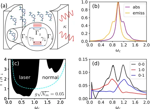
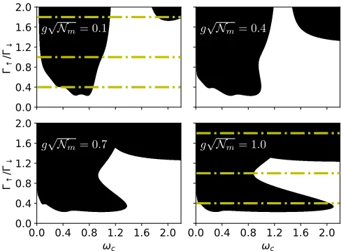
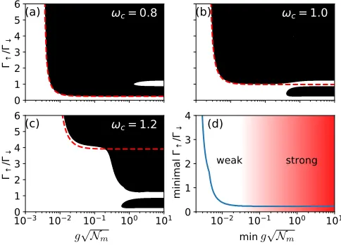
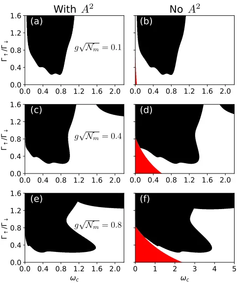
Artem Strashko,1 Peter Kirton,2 and Jonathan Keeling1
1SUPA, School of Physics and Astronomy, University of St Andrews, St Andrews, KY16 9SS, United Kingdom 2
Vienna Center for Quantum Science and Technology, Atominstitut, TU Wien, 1040 Vienna, Austria (Dated: October 22, 2018)
Following experimental realizations of room temperature polariton lasing with organic molecules, we present a microscopic model that allows us to explore the crossover from weak to strong matter-light coupling. We consider a non-equilibrium Dicke-Holstein model, including both strong coupling to vibrational modes and strong matter-light coupling, providing the phase diagram of this model in the thermodynamic limit. We discuss the mechanism of polariton lasing, uncovering a process of self-tuning, and identify the relation and distinction between regular dye lasers and organic polariton lasers.
Bose-Einstein statistics underpin both the thermal equilibrium phenomenon of Bose-Einstein condensation, and the non-equilibrium phenomenon of lasing. Lying be-tween these two extremes, there now exist several experi-mental platforms; in particular exciton-polaritons (quasi-particles resulting from strong coupling between photons and excitons) in semiconductor microcavities at cryo-genic temperatures [1–3], and photons in dye-filled micro-cavities at room temperature [4]. Since these microcavi-ties are imperfect, they are sources of coherent light (as is a laser), but differ in mechanism from photon lasing [5, 6]. Indeed, polariton lasing does not need electronic inver-sion, and so it is often stated that it can provide coherent light sources with ultra-low thresholds. Polariton lasing can also occur at room temperature in appropriate ma-terials: inorganic materials such as wide bandgap semi-conductors [7–9] and two-dimensional materials [10], and the focus of this Letter, organic materials [11–13].
Polariton condensation in organic materials prompts interesting questions regarding the mechanisms of po-lariton relaxation and lasing. Excitons in organic ma-terials are Frenkel excitons — electronic excitations of a molecule or chromophore delocalized by hopping [14]. Excitons in organic materials typically show complex ab-sorption and emission spectra, due to strong coupling be-tween the electronic state and the nuclear configuration, leading to rovibrational dressing. This causes a Stokes shift, so that emission is at longer wavelengths than ab-sorption. Spectral separation of emission and absorption underpins the operation of dye lasers [15], allowing gain without electronic inversion. Since both strong matter-light coupling and large Stokes shifts are expected to re-duce the lasing threshold, how they act in concert is of both fundamental interest and practical relevance.
Theoretical modeling of polariton condensates can fol-low a number of approaches. To describe the macro-scopic pattern formation and superfluid hydrodynam-ics it mostly suffices to use the phenomenological com-plex Gross-Pitaevskii equation [6, 16]. However, similar equations also apply for a photon laser [17, 18], so such approaches cannot be used to understand the relation between polariton and photon lasing, or the particular
properties of organic polaritons. To answer such ques-tions, a more relevant approach is to use kinetic equa-tions for the population of polaritons and excitonic reser-voir, with decay rates accounting for vibronically assisted processes [19–22] relevant in organic materials. This ap-proach has been used to understand the onset of lasing in anthracene microcavities [23] and J-aggregated dyes [24]. It however assumes polariton modes are well defined, so cannot access the weak- to strong-coupling crossover. In this Letter we will work from a microscopic Hamilto-nian which can, in the appropriate limit, recover both the physics described in such a kinetic model, as well as that of a dye laser in weak coupling.
We consider the non-equilibrium Dicke-Holstein model, presented below, which describes many molecules (with vibrationally dressed electronic transitions) cou-pled to a common photon mode. The equilibrium phase diagram of this model has been presented elsewhere [25]. Similar models have been used to understand the absorp-tion and photoluminescence spectra of organic polari-tons [26–29], and to explore whether strong matter-light coupling affects chemical reactions [30–32]. Despite this, the non-equilibrium dynamics of this model, when both photons and vibrations couple strongly to the electronic state, has not been explored. If coupling to vibrations is weak, one can eliminate these using Bloch-Redfield-Wangsness theory [33, 34] to capture the relaxation dy-namics. For weak coupling to light, rate equations are available [35–38], describing photon condensation. For a few molecules, one can use exact numerical methods, treating the vibrational modes as a non-Markovian dis-sipation process [39, 40]. However, the thermodynamic limit with many molecules and strong coupling remains a challenge, which we address here.
the practically significant question of whether strong cou-pling reduces lasing threshold, and the optimal parame-ters to realize polariton lasing.
0.0 0.4 0.8 1.2 1.6 2.0
c
0.00 0.05 0.10 0.15
(d) 0-0
1-0 0-1
0.0 0.5 1.0 1.5 2.0 0
1 2 3 4
Figure 1. (a) Cartoon illustrating our model: many molecules (N-level systems) are coupled to a cavity mode. (b-d) Weak coupling behavior. (b) Emission and absorption spectra of the molecules. (c) Weak coupling phase diagram. The cyan dashed line marks the phase boundary without vibrational dressing (S= 0). (d) Dominant molecular transitions coupled into the lasing mode at threshold. All energies are measured in units of ε ≡ 1, other parameters are S = 0.1, ωv = 0.2,
Γ↓=κ= 10−4, Γz= 0.03,γv= 0.02,kBTv= 0.025,Nv= 4.
We consider a single cavity mode, with frequency
ωc, coupled to Nm organic molecules as illustrated in Fig. 1(a). We model each molecule as two electronic states (HOMO and LUMO levels), dressed by a bosonic mode (describing a well-defined vibrational mode of the molecule) which is strongly coupled to the electronic state. This yields the Dicke-Holstein model:
H =X
n
n
εσnz+ωv
h b†nbn+
√
Sσzn(b†n+bn)io
+ωca†a+g a†+a
X
n
σxn+
g2Nm
ε (a
†+a)2, (1)
where σnα=x,y,z are Pauli matrices describing the elec-tronic state of molecule n,b†n creates a vibrational exci-tation on moleculen, anda†creates a photon. To explore the ultrastrong matter-light coupling regime we do not make a rotating-wave approximation and we include a diamagneticA2 term, which prevents a ground state su-perradiant transition (see [41–45]). We note the diamag-netic term could be eliminated by a Bogoliubov trans-form, yielding a model without theA2 term, but with a modified photon frequency ωeff
c =
p
ωc(ωc+ 4g2Nm/ε), and matter-light coupling geff = gp
ωc/ωceff. We char-acterize matter-light coupling by the “bare” polariton splitting g√Nm, which would be the splitting between the upper and lower polariton in the limitS→0.
To include incoherent pumping and decay processes, we use a Lindblad master equation [46] of the form:
˙
ρ(t) =−i[H, ρ] +κL[a] +X n
Γ↓L[σ−n] + Γ↑L[σn+]
+ ΓzL[σzn] +γ↑L[b†n−
√
Sσnz] +γ↓L[bn−
√ Sσzn]
, (2)
whereL[X] =XρX†−{X†X, ρ}/2. We include excitonic pumping and decay with rates Γ↑,Γ↓ respectively, and photon loss with rateκ. We also include dephasing of the electronic transition at rate Γz. The main source of this dephasing is the other molecular vibrational and rota-tional modes, weakly coupled to the electronic transition (in contrast to the strongly coupled mode included in the Hamiltonian). The final two terms describe relaxation of the vibrational mode to thermal equilibrium at tempera-tureTv, accounting for the electronic-state-dependent vi-brational displacement. These rates are thusγ↑=γvnB,
γ↓ = γv(nB + 1) where nB = [exp(ωv/kBTv)−1]−1. Throughout this Letter we measure energies in units of the electronic transition energy, so ε ≡ 1 by definition — typical physical values are ε ' 1–2eV — other pa-rameters are given in the caption of Fig. 1. We choose parameters that are physical and demonstrate side-peaks in the molecular spectra, Fig. 1(b). The resulting weak coupling phase diagram, Fig. 1(c), is straightforward to understand. The threshold Γth
↑ is reduced compared to the case without vibrational dressing (cyan line in Fig. 1(c)), and shows local mimima when the cavity fre-quency matches the emission side-peaks atωc < 1. In contrast Γth
↑ increases when the cavity matches the ab-sorption side-peaks forωc >1.
Our aim is to consider the large Nm limit of this model exactly, allowing both for strong matter-light cou-pling and strong coucou-pling between vibrational and elec-tronic states. In the large Nm limit, a mean-field (i.e. Maxwell-Bloch) treatment of the Dicke model becomes exact [47, 48]. There is however no decoupling between electronic and vibrational degrees of freedom. Instead we define generalized molecular operators, describing an
N-level system as a whole, with N = 2Nv forNv vibra-tional levels, where the choice ofNvdepends on the value ofS. We write the operators for thisN-level system us-ing a basis of generalized Gell Mann matrices λi [49], satisfying Tr(λiλj) = 2δij. This enables us to write any operator asO= (λi/2)Tr (Oλi) [50]. We may then write the Hamiltonian as:
H=ωca†a+
X
n
Ai+Bi(a†+a)
λ(in)+g 2N
m
ε (a
†+a)2,
[image:2.612.57.297.100.275.2]master equation can be rewritten in the same way:
˙
ρ(t) =−i[H, ρ] +κL[a] +X µn
Lhcµiλ(in)i. (4)
The sum over µ is over the five molecular dissipative channels in Eq. (2). If these terms are written as
P
µΓµL[Jµ] then we havecµi =
p
ΓµTr(Jµλi)/2.
The mean-field decoupling is realized by deriving the equations of motion for variables α = hai, `i = hλii, wherehOi= Tr(ρO), and thenassuminghaλii=haihλii
to give the coupled differential equations:
∂tα=−
iωc+
κ
2
α−4ig
2N m
ε Re[α]−iNmBi`i, (5) ∂t`i=
ξik+ 4fijkBjRe[α]
`k+
4i Nc
µ jc
µ∗
k fijk, (6)
where ξik = 2fijkAj+ic µ
lcµ∗m(filpζmpk+fmipζplk) with
ζijk≡Tr(λiλjλk)/2, andfijk≡Tr([λi, λj]λk)/4i. Mean-field theory shows a phase transition between a normal state with α= 0, and a state withα6= 0 which we denote as a laser but which may be either photon or polariton lasing. The phase boundary can be found by considering when fluctuations about the normal state are unstable. We thus write linearized equations of motion for fluctuationsα=δα,`i=`i,ns+δ`i, where`i,nsis the normal state solution. Definingυ= (δα, δα∗, δ`)|we can write∂tυ=Mυ, and find the eigenmodes,Mvk =ξkvk. The real part ofξk gives the growth (positive) or decay (negative) rate of a mode, while the imaginary part gives its oscillation frequency.
From the eigenvectorυk we can also find the contribu-tions of different molecular transicontribu-tions to the given un-stable mode (see [45] for details.) As an example of this, Fig. 1(d) shows the composition of the unstable mode precisely at the lasing threshold, i.e. along the phase boundary shown in Fig. 1(c). We see that where the threshold is low, the (1–0) transition contributes most, while where the threshold is high, the (0–1) transition dominates. In this Letter we show results with up to three vibrational excitations, i.e.N= 8. Our results are converged for this choice as shown in [45].
Using the methods above, we now explore how strong coupling to light modifies the phase diagram, and un-derstand the physics responsible for this modification. Figure 2 shows the evolution of theωc,Γ↑ phase diagram as matter-light coupling increases, focusing on the low pumping regime. At moderate coupling, g√Nm = 0.1, we see the same form as for weak coupling, with a min-imum (maxmin-imum) threshold atωc 'ε∓ωv. Asg
√ Nm increases, the most striking feature is that the lobe at
ωc ≈ ε−ωv bends and, at weak pumping, extends to significantly higher cavity frequencies. This eventually leads to a re-entrant phase diagram.
To understand the origin of this extension of the lobe to high cavity frequencies, we explore the nature of the
un-Figure 2. Evolution of phase diagrams with increasing cou-pling,g√Nm (values as shown). Dash-dotted (yellow) lines indicate the cuts shown in Fig. 3. Parameters as in Fig. 1.
stable mode. Figure 3 shows the composition of the un-stable mode, and the frequency of all modes for three cuts across the phase diagram at fixed pump power at weaker and stronger coupling. For orientation, we first summa-rize the more straightforward behavior seen at weaker coupling, g√Nm = 0.1. In Fig. 3(a), for low pumping Γ↑ = 0.4Γ↓, the frequencies of the normal modes show a small polaritonic splitting where the effective photon frequency [51] crosses molecular transitions, most clearly the zero phonon line at Im[ξ] =ε≡1, i.e the (0–0) tran-sition. Lasing occurs when the bare photon frequency is close to the (1-0) or (2-0) transitions (but with differ-ent strengths for these two transitions). Indeed, as seen in Fig. 3(d), the unstable mode predominantly involves the (1–0) transition, crossing over to the (0–0) transi-tion asωc approaches the zero phonon line. As pumping increases to Γ↑ = Γ↓, Fig. 3(b,e), saturation suppresses the polariton splitting, and lasing is possible over a wider range of frequencies. Finally, at Γ↑= 1.8Γ↓, Fig. 3(c,f), excitonic pumping exceeds decay, so we have electronic inversion, and can achieve lasing even where the absorp-tion spectrum exceeds emission. Here we have two lasing regions at low and high frequencies. At yet higher pump strengths, these regions join.
[image:3.612.317.561.50.230.2]Figure 3. Nature of lasing instability. Top (a–c,g–i): Real (right, solid cyan) and imaginary (left, grayscale) parts of linearized eigenvaluesξ. The grayscale indicates the photon component of that mode. The yellow dashed line highlights which imaginary part corresponds to the mode that is unstable (i.e has a positive real part). The pink dotted line shows the effective photon frequency,ωeffc . Bottom (d–f, j–l): Vibrational composition of unstable mode. Parameters as in Fig. 1.
As pumping increases to Γ↑ = Γ↓, the polaritonic self-tuning effect reduces and we no longer have lasing over such a wide range of cavity frequencies. As noted above, stronger pumping suppresses the polaritonic split-ting, and this prevents the self-tuning effect(similar sup-pression of effective matter-light coupling is caused by increasing the dephasing rate Γz, see [45]). We nonethe-less still have notable polaritonic splitting at low cavity frequencies. The molecular transitions involved in las-ing in Fig. 3(k) is similar to that in Fig. 3(e), but now (0–1) and (1–1) transitions play a larger role, as strong coupling admixes more electronic transitions into the po-lariton. As we further increase pumping to Γ↑ = 1.8Γ↓ we now have two distinct lasing regimes: at low cavity frequency, there is polariton lasing, but at high cavity frequencies, lasing is at the bare cavity photon frequency (see [45] for an extended figure).
Having analyzed the structure of the phase diagram, we next consider whether strong matter-light coupling is a direct route to reduce the lasing threshold. In Fig. 4(a– c) we plot phase diagrams vs Γ↑andg
√
Nmat three dif-ferent bare photon frequencies, and we compare these to the phase boundary predicted by weak coupling theory, see [45] for details. In all cases, we see the threshold reduce with increasing coupling. For cavity frequencies near the (1-0) transition, Fig. 4(a), the weak coupling prediction of the phase boundary matches the full re-sults well. For this optimal frequency, while threshold pumping does reduce with increasing coupling, it satu-rates as the system enters the strong coupling regime (where g√Nm is larger than the linewidth Γz).
How-ever, for cavity frequencies near theabsorption side-peak at the (0-1) transition, Fig. 4(c), one sees the full cal-culation predicts a dramatically lower threshold than is predicted by weak coupling, and the threshold continues to reduce even after entering the strong coupling regime. In Fig. 4(d) we summarize the data by plotting the minimal pumping strength (optimized over cavity
fre-Figure 4. (a-c) Phase diagrams at various cavity frequencies. Red dashed line shows the weak-coupling theory phase bound-ary, see [45]. (d) Minimal critical pump strength (optimized over cavity frequency) as a function of matter-light coupling. Red shading indicates weak- to strong-coupling crossover.
[image:4.612.317.559.269.443.2]Further, considering a multimode Dicke model, one can study thermalization of mode populations, analogous to that seen for weak-coupling photon BEC [4, 35–38, 55]. Finally, one may consider more complex models, combin-ing multiple vibrational modes in the system, or uscombin-ing Redfield theory with the true system eigenstates to bet-ter capture the physics of structured baths, leading to a more realistic master equation [56, 57]. This may allow one to capture physics otherwise requiring numerically intensive non-Markovian simulations [39, 40]. Together, these provide an efficient route to understand the full range of weak and strong matter-light coupling for po-lariton condensation and lasing.
AS acknowledges support from the EPSRC CM-CDT (EP/L015110/1). JK and PK acknowledges financial support from EPSRC program ”Hybrid Polaritonics” (EP/M025330/1). PK acknowledges support from the Austrian Academy of Sciences ( ¨OAW).
[1] H. Deng, G. Weihs, C. Santori, J. Bloch, and Y. Ya-mamoto, Condensation of Semiconductor Microcavity Exciton Polaritons, Science298, 199 (2002).
[2] J. Kasprzak, M. Richard, S. Kundermann, A. Baas, P. Jeambrun, J. Keeling, F. Marchetti, M. Szyma´nska, R. Andre, J. Staehli, et al.,Bose–Einstein condensation of exciton polaritons, Nature443, 409 (2006).
[3] R. Balili, V. Hartwell, D. Snoke, L. Pfeiffer, and K. West, Bose-Einstein Condensation of Microcavity Polaritons in a Trap, Science316, 1007 (2007).
[4] J. Klaers, J. Schmitt, F. Vewinger, and M. Weitz,Bose– Einstein condensation of photons in an optical microcav-ity, Nature468, 545 (2010).
[5] H. Deng, H. Haug, and Y. Yamamoto,Exciton-polariton Bose-Einstein condensation, Rev. Mod. Phys. 82, 1489 (2010).
[6] I. Carusotto and C. Ciuti,Quantum fluids of light, Rev. Mod. Phys.85, 299 (2013).
[7] S. Christopoulos, G. B. H. von H¨ogersthal, A. J. D. Grundy, P. G. Lagoudakis, A. V. Kavokin, J. J. Baum-berg, G. Christmann, R. Butt´e, E. Feltin, J.-F. Carlin, and N. Grandjean, Room-Temperature Polariton Lasing in Semiconductor Microcavities, Phys. Rev. Lett. 98, 126405 (2007).
[8] T. Guillet, M. Mexis, J. Levrat, G. Rossbach, C. Bri-mont, T. Bretagnon, B. Gil, R. Butt´e, N. Grandjean, L. Orosz, et al., Polariton lasing in a hybrid bulk ZnO microcavity, Appl. Phys. Lett.99, 161104 (2011). [9] F. Li, L. Orosz, O. Kamoun, S. Bouchoule, C.
Bri-mont, P. Disseix, T. Guillet, X. Lafosse, M. Ler-oux, J. Leymarie, M. Mexis, M. Mihailovic, G. Patri-arche, F. R´everet, D. Solnyshkov, J. Zuniga-Perez, and G. Malpuech,From Excitonic to Photonic Polariton Con-densate in a ZnO-Based Microcavity, Phys. Rev. Lett. 110, 196406 (2013).
[10] M. Waldherr, N. Lundt, M. Klaas, S. Betzold, M. Wurdack, V. Baumann, E. Estrecho, A. Nalitov, E. Cherotchenko, H. Cai, E. A. Ostrovskaya, A. V. Ka-vokin, S. Tongay, S. Klembt, S. Hfling, and C. Schneider,
Observation of bosonic condensation in a hybrid mono-layer MoSe2-GaAs microcavity, (2018), 1805.03630. [11] S. K´ena-Cohen and S. Forrest,Room-temperature
polari-ton lasing in an organic single-crystal microcavity, Nat. Photon.4, 371 (2010).
[12] J. D. Plumhof, T. St¨oferle, L. Mai, U. Scherf, and R. F. Mahrt, Room-temperature Bose–Einstein conden-sation of cavity exciton–polaritons in a polymer, Nature materials13, 247 (2014).
[13] K. Daskalakis, S. Maier, R. Murray, S. K´ena-Cohen, et al.,Nonlinear interactions in an organic polariton con-densate, Nat. Mater13, 271 (2014).
[14] V. M. Agranovich,Excitations in organic solids(Oxford University Press, Oxford, 2009).
[15] F. P. Sch¨afer, ed.,Dye Lasers, 3rd ed. (Springer-Verlag, Berlin, 1990).
[16] I. S. Aranson and L. Kramer, The world of the com-plex Ginzburg-Landau equation, Rev. Mod. Phys. 74, 99 (2002).
[17] K. Staliunas and V. J. Sanchez-Morcillo,Transverse pat-terns in nonlinear optical resonators, Vol. 183 (Springer-Verlag, Berlin, 2003).
[18] N. G. Berloff and J. Keeling, Universality in Modelling Non-equilibrium Pattern Formation in Polariton Con-densates, in Physics of Quantum Fluids: New Trends and Hot Topics in Atomic and Polariton Condensates, edited by A. Bramati and M. Modugno (Springer Berlin Heidelberg, Berlin, Heidelberg, 2013) pp. 19–38. [19] P. Michetti and G. C. La Rocca,Exciton-phonon
scatter-ing and photoexcitation dynamics in J-aggregate micro-cavities, Phys. Rev. B79, 035325 (2009).
[20] L. Fontanesi and G. C. La Rocca,Organic-based micro-cavities with vibronic progressions: Linear spectroscopy, Phys. Rev. B80, 235313 (2009).
[21] L. Mazza and G. C. La Rocca,Organic-based microcavi-ties with vibronic progressions: Photoluminescence, Phys. Rev. B80, 235314 (2009).
[22] P. Michetti, L. Mazza, and G. C. La Rocca, Organic Nanophotonics, Nano-Optics and Nanophotonics, edited by Y. S. Zhao (Springer, Berlin, 2015).
[23] L. Mazza, S. K´ena-Cohen, P. Michetti, and G. C. La Rocca, Microscopic theory of polariton lasing via vi-bronically assisted scattering, Phys. Rev. B 88, 075321 (2013).
[24] D. M. Coles, P. Michetti, C. Clark, W. C. Tsoi, A. M. Adawi, J.-S. Kim, and D. G. Lidzey, Vibrationally As-sisted Polariton-Relaxation Processes in Strongly Cou-pled Organic-Semiconductor Microcavities, Adv. Funct. Mater.21, 3691 (2011).
[25] J. A. ´Cwik, S. Reja, P. B. Littlewood, and J. Keeling, Polariton condensation with saturable molecules dressed by vibrational modes, Europhys. Lett.105, 47009 (2014). [26] J. A. ´Cwik, P. Kirton, S. De Liberato, and J. Keeling, Excitonic spectral features in strongly coupled organic po-laritons, Phys. Rev. A93, 033840 (2016).
[27] F. Herrera and F. C. Spano, Dark Vibronic Polaritons and the Spectroscopy of Organic Microcavities, Phys. Rev. Lett.118, 223601 (2017).
[28] F. Herrera and F. C. Spano,Theory of nanoscale organic cavities: The essential role of vibration-photon dressed states, ACS Photonics5, 65 (2017).
5, 249 (2017).
[30] F. Herrera and F. C. Spano,Cavity-Controlled Chemistry in Molecular Ensembles, Phys. Rev. Lett. 116, 238301 (2016).
[31] J. Feist, J. Galego, and F. J. Garcia-Vidal, Polaritonic chemistry with organic molecules, ACS Photonics5, 205 (2017).
[32] R. F. Ribeiro, L. A. Mart´ınez-Mart´ınez, M. Du, J. Campos-Gonzalez-Angulo, and J. Y. Zhou,Polariton Chemistry: controlling molecular dynamics with optical cavities, Chem. Sci.9, 6325 (2018).
[33] R. K. Wangsness and F. Bloch,The Dynamical Theory of Nuclear Induction, Phys. Rev.89, 728 (1953). [34] A. G. Redfield,Nuclear Magnetic Resonance Saturation
and Rotary Saturation in Solids, Phys. Rev. 98, 1787 (1955).
[35] P. Kirton and J. Keeling,Nonequilibrium Model of Pho-ton Condensation, Phys. Rev. Lett.111, 100404 (2013). [36] P. Kirton and J. Keeling,Thermalization and breakdown of thermalization in photon condensates, Phys. Rev. A 91, 033826 (2015).
[37] H. J. Hesten, R. A. Nyman, and F. Mintert, Deconden-sation in Nonequilibrium Photonic Condensates: When Less Is More, Phys. Rev. Lett.120, 040601 (2018). [38] M. Radonji´c, W. Kopylov, A. Balaˇz, and A. Pelster,
Interplay of coherent and dissipative dynamics in con-densates of light, New J. Phys.20, 055014 (2018). [39] J. del Pino, F. A. Schr¨oder, A. W. Chin, J. Feist,
and F. J. Garcia-Vidal, Tensor network simulation of non-Markovian dynamics in organic polaritons, (2018), 1804.04511.
[40] J. del Pino, F. A. Schr¨oder, A. W. Chin, J. Feist, and F. J. Garcia-Vidal, Tensor Network simulation of polaron-polaritons in organic microcavities, (2018), 1807.00586.
[41] K. Hepp and E. H. Lieb,Equilibrium statistical mechan-ics of matter interacting with the quantized radiation field, Phys. Rev. A8, 2517 (1973).
[42] K. Rza˙zewski, K. W´odkiewicz, and W. ˙Zakowicz,Phase transitions, two-level atoms, and the A 2 term, Phys. Rev. Lett. 35, 432 (1975).
[43] T. Grießer, A. Vukics, and P. Domokos,Depolarization shift of the superradiant phase transition, Phys. Rev. A
94, 033815 (2016).
[44] D. De Bernardis, T. Jaako, and P. Rabl,Cavity quan-tum electrodynamics in the nonperturbative regime, Phys. Rev. A97, 043820 (2018).
[45] See Supplemental Material for discussion of theA2term, further details of the linear stability calculation, con-vergence with number of vibrational states, dependence on vibrational frequency and damping rates,and further analysis of the phase diagrams presented.
[46] H.-P. Breuer and F. Petruccione, The Theory of Open Quantum Systems (Oxford University Press, Oxford, 2002).
[47] H. Haken,The semiclassical and quantum theory of the laser, inQuantum Opt., edited by S. M. Kay and A. Mait-land (1970) p. 201.
[48] P. Kirton and J. Keeling,Suppressing and Restoring the Dicke Superradiance Transition by Dephasing and Decay, Phys. Rev. Lett.118, 123602 (2017).
[49] M. Stone and P. Goldbart,Mathematics for physics: a guided tour for graduate students(Cambridge University Press, Cambridge, 2009).
[50] In writing this, we have definedλ0= (2/N)1N.
[51] i.e. this line plots the quantity pωc(ωc+ 4g2Nm/ε),
hence its nonlinear dependence onωcat strong coupling.
[52] D. Meiser, J. Ye, D. R. Carlson, and M. J. Holland, Prospects for a Millihertz-Linewidth Laser, Phys. Rev. Lett.102, 163601 (2009).
[53] D. Meiser and M. J. Holland, Intensity fluctuations in steady-state superradiance, Phys. Rev. A 81, 063827 (2010).
[54] P. Kirton and J. Keeling,Superradiant and lasing states in driven-dissipative Dicke models, New J. Phys. 20, 015009 (2018).
[55] J. Marelic and R. A. Nyman,Experimental evidence for inhomogeneous pumping and energy-dependent effects in photon Bose-Einstein condensation, Phys. Rev. A 91, 033813 (2015).
[56] C. Ciuti, G. Bastard, and I. Carusotto,Quantum vacuum properties of the intersubband cavity polariton field, Phys. Rev. B72, 115303 (2005).
SUPPLEMENTARY MATERIAL FOR: ”ORGANIC POLARITON LASING AND THE WEAK- TO STRONG-COUPLING CROSSOVER”
ROLE OF DIAMAGNETICA2 TERM
This section discusses the role of the diamagnetic A2 term, allowing one to disentangle the effects of this term vs other effects of strong coupling on the form of the phase diagram.
As noted in the text, thisA2 term is included in order to avoid a ground-state superradiant transition, following the results of Rza˙zewskiet al.[42]. Without the diamag-netic term, the ground state of the Dicke model at strong coupling is a state with a macroscopic occupation of the photon [41], even in the absence of pumping. The inclu-sion of theA2 term, with a coefficient determined by the oscillator strength sum rule prevents this transition oc-curring [42], so the ground state remains stable at all cou-pling strengths. Recently the question of whether a phase transition is in fact possible in the ground state has been re-opened, with a consensus developing that a transition is possible, but driven by dipole-dipole interactions be-tween atoms when in the appropriate geometry [43, 44]. We neglect the possibility of this ferromagnetic transition here, and include anA2term so that only the transition induced by incoherent pumping is present.
[image:7.612.55.297.381.668.2]With No
Figure S1. Role of A2 term, fixed coupling, parameters as in Fig. 1. White region denotes normal state, black denotes lasing, and red the superradiant phase. Note the different x-axis scale in panel (f).
Figure S1 compares the phase diagrams (vs bare cavity frequency and pumping) with (left) and without (right) the diamagneticA2 term. In the phase diagrams with-out the A2-term a superradiant phase is present at low photon frequencies and low pumping. As discussed else-where [54], this superradiant state can be distinguished from the lasing state by the nature of the instability and the spectrum of the emission: ground state superradi-ance is a stationary steady state, while the lasing state is at finite frequency, and thus is time dependent in the lab frame. As a consequence, the superradiant state instability involves a single unstable frequency (regions marked red on Fig. S1), while the lasing state instabil-ity involves a complex conjugate pair of unstable modes (regions marked black on Fig. S1).
Regarding the effect of the A2 term on the shape of the polariton lasing region, we see from Fig. S1 that the lasing phase remains a similar shape, although the char-acteristic frequency ranges are significantly rescaled at strong coupling. As pointed out in the Letter, the A2 term has a twofold effect. Firstly, it leads to renormal-ization of the effective photon frequencyωeff
c , which leads to ag-dependent effective detuning. Secondly, it reduces the effective exciton-photon coupling. In the ultrastrong coupling shown in Fig. S1(e,f), the combination of these effects results in the effective decoupling of the photon from the molecular excitations, causing the lasing region to shrink to a significantly lower frequency range. As the shape is similar, we can be clear the bending of the lasing lobe is not associated with theA2 term.
EFFECT OF VIBRATIONAL TRUNCATION
In Fig. S2 we show the dependence of the phase dia-gram on the number of vibrational statesN. We show results for S = 0.1 and for two values of matter-light coupling, g√Nm = 0.1 and g
√
Nm = 1.0, correspond-ing to the top left and bottom right panels of Fig. 2 in which we used Nv = 4. For the weaker coupling,
g√Nm= 0.1, asNv increases the phase diagram retains a similar structure, but one can see the appearance of new peaks at ωc ≈0.6,0.4,0.2 corresponding to (2-0), (3-0) and (4-0) transitions respectively. For stronger coupling,
g√Nm= 1.0, we see a similar emergence of extra peaks, and a slight evolution of the extended lasing lobe. In both cases we see that the results do not differ signifi-cantly between Nv = 4 and Nv = 5, confirming we can safely useNv= 4 in our Letter.
Figure S2. Dependence of phase diagrams on the number of vibrational levels retained,Nv. Other parameters as in Fig. 1.
isPn =e−SSn/n!, thus forS= 0.1, we would expect re-sults to be dominated byn= 0,1. The behavior shown in Fig. S2 shows that despite this, higher vibrational states do play some role even for these small values ofS.
EFFECT OF VIBRATIONAL PROPERTIES ON PHASE DIAGRAM
In this section we show how the frequency and deco-herence rates of the vibrational mode affect the phase diagram at strong matter-light coupling
Effect of vibrational damping rate
Since the self-tuning that leads to the extension of the lasing region to high cavity frequencies requires strong coupling, we expect that incoherent processes (which suppress strong coupling) will reduce the self tuning. To check this, in Fig. S3 we show phase diagrams for very
Figure S3. Dependence of phase diagram atg√Nm= 1.0 on
varying vibrational dampingγvand excitonic dephasing rate
Γz.
strong couplingg√Nm= 1.0, varying the relaxation rate of the vibrational mode γv and the excitonic dephasing Γz. Increasing either of these quantities leads to a similar effect on the phase diagram: The size of the entrant re-gion, associated with the self-tuning effect, reduces. Both of these quantities lead to extra dephasing of the molecu-lar states, this reduces the effective matter-light coupling and hence suppresses the self-tuning effect.
Effect of vibrational frequency
In Fig. S4 we explore the effect of changing the fre-quency of the vibrational mode. We plot the phase dia-grams and spectrum at the pump strengths correspond-ing to the maximal range of self-tuncorrespond-ing, in the strong cou-pling regime,g√Nm = 1.0, for ωv = 0.1,0.2,0.3. From these figures we can observe that the bending of the low pumping lasing peak and re-entrant behavior is present at allωv. We thus see that the existence of the self-tuning effect is independent of the mode frequency. However, as expected, the self-tuned lower polariton frequency moves to follow the vibrational sideband.
The shape and extent of the lasing peak does however change with vibrational frequency. Notably, the peak extends to the highest cavity frequencies at small ωv, but extends to the lowest pump strength at large ωv. The behavior at small ωv can be understood as a re-sult of the vibrational sidebands becoming less well de-fined as the vibrational frequency approaches the inco-herent linewidth. At largeωv, there is a reduction in the effective matter-light coupling strength, due to polaron formation [29, 30], however the parameters chosen here are always in the regime where the re-organization en-ergy ωvS is smaller than the Rabi splitting g
√
[image:8.612.54.298.51.423.2]Figure S4. Phase diagrams and spectrum atg√Nm= 1.0 for
different vibrational frequencies.
as discussed in Ref. [29], polaron formation is strongly suppressed.
NATURE OF THE LASING INSTABILITY
In this section we provide further details on the calcu-lation of the vibrational composition of the lasing mode, and present figures illustrating the evolution of the spec-trum.
Composition of linear stability eigenmodes
To determine the molecular transitions corresponding to a given unstable mode, we note that from the eigen-vector υ = (δα, δα∗, δ`)| of the stability matrix M, we can extract the matter part δ`i and so construct the corresponding molecular density matrix, ρ(t) = ρns + A(δ`ieξt+δ`∗ieξ
∗t
)λi/2 where A is an arbitrary ampli-tude and ρns is the normal state density matrix. (For simplicity of notation, we neglect the superscripts onδ`
and ξ labeling eigenmodes.) The complex conjugates appearing here are required in order to guarantee Her-miticity (given the Gell Mann matrices are defined to be Hermitian). This step is crucial since the equations of motion mix `i and `∗i. To find the amplitude of the oscillatory component of a given element of the density matrix ρij, we first define the matrix r = δ`iλi/2 and then note the oscillatory component ofρijtakes the form
δρij =rijeξt+r∗jieξ ∗t
.
While the diagonal components of a density matrix give the molecular state populations, nondiagonal ones correspond to coherences. In particular, the block of the density matrix which is off-diagonal in terms of electronic states gives the weights of molecular transi-tions involved in lasing. For the diagonal components of the density matrix we can immediately write δρii = 2|rii|cos ξ00t+ Arg(rii)eξ
0t
whereξ0, ξ00denote real and imaginary parts of the eigenvalue respectively. For the off diagonal components, the behavior is more complex
as in general|rij| 6=|rji|; we thus expect that the quan-tity δρij traces an elliptical spiral in the Argand plane,
δρij = [rAcos(ξ00t+φ) +irBsin(ξ00t+φ)]eiθ+ξ 0t
. One may readily show that the semi-major and semi-minor axes of this ellipse are given byrA,B=|rij| ± |rji|, while
φ, θ= [Arg(rij)±Arg(rji)]/2. Given this behavior, we define the amplitude of a given component by the semi-major axis. The contribution of a given molecular tran-sition (n−m) to the lasing mode thus corresponds to the amplitude|rn↓,m↑|+|rm↑,n↓|.
Evolution of spectrum with coupling
In Fig. 3 we showed the evolution of the spectrum with increasing pumping. Here, in Fig. S5, we complement this by showing how the spectrum evolves with increas-ing matter-light couplincreas-ing at weak pumpincreas-ing. We clearly see how the polariton splitting increases and self-tuning develops with increasing coupling. We may also note that the real part of the unstable eigenvalue increases, so the lasing instability will develop on a shorter timescale.
Figure S5. Evolution of spectrum as coupling g√Nm in-creases, for weak pumping Γ↑= 0.4Γ↓. Line colors and styles
as in Fig. 3, parameters as in Fig. 1.
Transition from polariton to photon lasing
In Fig. S6 we show the spectrum for the same parame-ters as in Fig. 3(i) (strong coupling and strong pumping), but over an extended axis range.This figure illustrates the transition between the two different lasing states which occurs in this regime. For low cavity frequencies (around
ωc . 1.5) the system supports self-tuning and we get polariton lasing. However at larger cavity frequencies, the larger detuning in combination with strong pumping suppresses strong coupling leading to “normal” lasing at effective photon frequencyωeff
[image:9.612.317.560.326.486.2]rate for this second lasing instability is much slower than in the polariton lasing regime.
We note that in this figure, because we use Nv = 4, we see only a limited range of vibrational sidebands. A calculation with largeNvwould show a sequence of side-bands up to higher frequency (but with a weight that decreases as one goes to higher frequencies).
Figure S6. Spectrum for g√Nm = 1.0, Γ↑ = 1.8Γ↓ on an
enlarged axis. Line colors and styles as in Fig. 3, parameters as in Fig. 1.
PHASE BOUNDARY VS COUPLING STRENGTH
In this section we discuss further the phase boundaries and minimum lasing threshold shown in Fig. 4. We pro-vide further cuts of the phase diagram at different cavity frequencies, present the optimal cavity frequency at a given coupling strength, and provide details of the weak coupling calculation that is shown in Fig. 4(a-c).
Evolution of phase boundary with cavity frequency
We first provide further detail on the how the phase boundary evolves with cavity frequency. Figure 4(a-c) presents the phase diagrams at three specific frequencies; to show more clearly how the phase boundary evolves with frequency, the top panel of Fig. S7 shows a sequence of curves, giving the evolution of the phase boundary with bare photon frequency. Note that the phase bound-ary has different topology forωc ≤0.9 andωc ≥1. For low frequency, there is a single lasing region (but with a hole appearing at large coupling around Γ↑ ' Γ↓). Around ωc = 1, this hole reaches the phase boundary, dividing the lasing region into two: a large region at high pumping, and a smaller region, below inversion and at strong coupling.
0.6 0.7 0.8 0.9 1.0 1.1 1.2 0
1 2 3 4 5
critical
[image:10.612.318.560.49.295.2]/
Figure S7. Top: Critical pump strength as a function of cou-pling strength for various bare cavity frequenciesωc. Bottom:
The cavity frequenciesωc at which the threshold has a local
minimum as a function of couplingg√Nm. The thick gray line highlights which frequency corresponds to the global min-imum. Parameters as in Fig. 1.
Optimal cavity frequency
The lower panel of Fig. S7 shows the cavity frequen-cies at which the threshold has local minima. As could already be seen in Fig. 2, the threshold shows multiple local minima at vibronic replicasωc =ε−nωv. At the lowest coupling, the minimal threshold is nearωc=ε be-cause this corresponds to the peak emission — for very low coupling, the critical condition is for emission to beat cavity loss. Note that the threshold lasing power diverges aroundg√Nm'0.0024, i.e. for the parameters we use, there is no lasing at weaker coupling than this. When coupling increases to g√Nm ≈ 0.0035, we get another local minimum emerging atωc≈ε−ωv corresponding to the (1-0) transition. For g√Nm &0.004 this new min-imum becomes the global minmin-imum, i.e. it leads to the lowest threshold pumping as shown in Fig. 4(d). As we enter strong coupling regime g &0.03 we get one more local minimum driven by (2-0) transition and then an-other one due to (3-0) transition. All these local minima of pumping can be seen in Fig. 2.
[image:10.612.55.295.147.328.2]cou-pling, i.e. self-tuning allows the lasing threshold for this transition to move out to high cavity frequencies. In contrast, the (2-0) and (3-0) transitions do not show any strong-coupling self-tuning effect — the lasing transitions at these frequencies appear similar to weak coupling las-ing. The reason these lasing frequencies shift to lower frequencies is the renormalization of effective photon fre-quency by theA2 term. i.e., the resonance condition is in fact ωeff
c ' ε−nωv, and the dependence of ωceff on
g√Nm means the resonance moves to lower bare cavity frequencies as coupling increases.
In the ultrastrong coupling regime, the (1-0) and (2-0) branches give almost the same threshold pumping around Γth↑ ≈ 0.22Γ↑, while the (3-0) transition has Γth
↑ ≈0.38Γ↑, as can also be seen in Fig. 2.
Comparison to weak coupling theory
In Fig. 4, we compared the strong coupling phase dia-gram to a weak coupling prediction of the phase bound-ary. Here we provide details of this weak coupling pre-diction. The weak coupling theory of the Dicke-Holstein model has been discussed in Ref. [35, 36]. In those works, it is shown that treating matter-light coupling perturba-tively, one can derive a weak coupling master equation:
˙
ρ(t) =−ihH˜0, ρ
i
+κL[a] +X n
Γ↓L[σn−] + Γ↑L[σ+n]
+ ΓEL[a†σ−] + ΓAL[aσ+]
ρ, (S1)
where the free Hamiltonian is ˜H0= (ωc−ε)a†aand the rates of emission and absorption processes are given by
ΓA,E =g2
Z ∞
−∞
dte±iωcthσ−(t)σ+(0)i0. (S2)
The two-time correlation functionh. . .i0is calculated for free molecules, neglecting the matter-light coupling. In
Refs. [35, 36], a different form of dissipation was assumed for the vibrational modes, allowing an explicit form for ΓA,E through a Keldysh path integral. The form of dis-sipation considered here and written in Eq. (2) does not allow such a form, however the integrals in ΓA,E can be numerically calculated from the master equation using the quantum regression theorem [46].
From this equation, we can use the same mean-field decoupling discussed earlier, i.e. haσ±i = haihσ±i and ha†ai=|hai|2 to yield a set of non-linear coupled equa-tions:
∂thai= Nm
4
h
ΓA(1− hσzi)−ΓE(1 +hσzi)
i
hai
−hi(ωc−ε) +
κ
2
i
hai, (S3)
∂thσzi=
1− hσziΓ↑+ ΓA|hai|2
−1 +hσziΓ↓+ ΓE|hai|2
. (S4)
We can then again consider linear stability of the normal state, by considering fluctuations hai = α and hσzi = hσzins+z as in the Letter. One may see that α and
z are uncoupled, so the corresponding equations can be solved trivially, and the linearized eigenvalue is given by
ξ=−i(ωc−)−
κ
2+ Nm
4 (ΓE−ΓA)+ Nm
4 (ΓE+ΓA)hσ z
ins,
(S5) where hσzi
ns = (Γ↑−Γ↓)/(Γ↑+ Γ↓). One can extract threshold pumping as a function of couplingg, by solving Re[ξ] = 0, which gives:
Γth↑ = NmΓA+κ NmΓE−κ