Level set Cox processes
Anders Hildeman1, David Bolin1, Jonas Wallin2, and Janine B. Illian3 1Department of Mathematical Sciences, Chalmers University of Technology and
University of Gothenburg, Sweden
2Department of Statistics, Lund University, Sweden
3School of Mathematics and Statistics, University of St Andrews, Scotland, UK
Abstract
An extension of the popular log-Gaussian Cox process (LGCP) model for spatial point patterns is proposed for data exhibiting fundamentally dierent behaviors in dierent sub-regions of the spatial domain. The aim of the analyst might be either to identify and classify these regions, to perform kriging, or to derive some properties of the parameters driving the random eld in one or several of the subregions. The extension is based on replacing the latent Gaussian random eld in the LGCP by a latent spatial mixture model specied us-ing a categorically valued random eld specied through level set operations on a Gaussian random eld. This allows for standard stationary covariance structures, such as the Matérn family, to be used to model random elds with some degree of general smoothness but also occasional and structured sharp discontinuities.
A computationally ecient MCMC method is proposed for Bayesian inference and we show consistency of nite dimensional approximations of the model. Finally, the model is tted to point pattern data derived from a tropical rainforest on Barro Colorado island, Panama. We show that the proposed model is able to capture behavior for which inference based on the standard LGCP is biased.
1 Introduction
Cox processes, and in particular log-Gaussian Cox processes (LGCP), have been used extensively as exible models of spatial point pattern data [39, 38, 31, 20]. These are hierachical point process models where the point locations are assumed to be independent given a random intensity function
λ(s) = exp{B(s)β+ X(s)}, (1)
where B(s) is a, possibly multivariate, function of covariates and X(s) is a Gaussian random
eld, which is typically assumed to be stationary. The random eld captures spatial structure in the point pattern that the given covariates cannot capture. In this work, we relax the assumption that a single stationary Gaussian eld can account for those remaining spatial structures and develop a mixture model based on level set inversion.
To motivate the relevance of the approach we consider a point pattern data set formed by the locations of the tree species Beilschmiedia Pendula, one of the species in the tropical rainforest plot on Barro Colorado Island [12, 14, 10, 28]. The point pattern comprises2461point locations
in a rectangular observation window (500 m ×1000 m), see Figure 1a. This pattern has been
(a) (b) (c)
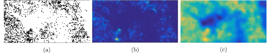
Figure 1: Spatial point pattern formed by the locations of trees of the species Beilschmiedia pendula in a 500 m×1000 m rainforest plot on Barro Colorado Island (a), a gridded version of
the data (b), and posterior mean of log intensity using a log-Gaussian Cox process model (c).
data sets to draw conclusions on the association of habitat preferences based on a number of spatial covariates reecting local soil chemistry and topography [38, 31].
On close inspection, the pattern shows large areas of very low point intensity where hardly any trees can be found. Anecdotal knowledge reveals that these regions are covered by a swamp, where the tree species is known to be very unlikely to grow, independent of local soil covariates and topography. However, data on the exact extent of the swamp is not available. We initially tted a log Gaussian Cox process to the data, with an intensity function as in (1) using 11
covariates, and the estimated posterior mean of the model also predicts large regions of low intensity, as plotted in Figure 1c. However, when a LGCP model that ignores the presence of swamp is tted to this pattern, the swamp is likely to act as a confounding factor and this is likely to impact on inference. Hence, any conclusions on habitat preferences of the species will be heavily biased. Covariates associated with the presence of the swamp may appear to have a signicant correlation with the intensity of the tree growth, or important covariates might appear non-signicant as they vary indepedently of the presence of the swamp.
The approach we take here is designed to capture sharp discontinuities in the intensity surface that result from qualitative yet unavailable covariates or environmental conditions as the one seen in this example. Further examples where this approach could be important is ecological data with several distinct types of habitat, spatial regions with dierent treatment regimes in medical data, or nding regions of interest in biology [23]. Specically, we consider a Cox process model where the intensity surface is modeled using a Bayesian level set approach. The proposed model is an extension of the log-Gaussian Cox process with increased exibility resulting from a random segmentation of the spatial region intoK classes. The intensity surfaces of the regions associated with theK dierent classes can be modeled separately of each other by log-Gaussian random elds with simple covariance structures, while still maintaining exibility. We refer to the proposed model as the level set Cox process (LSCP).
Finding sharp discontinuities in the intensity surface is similar to the level set inversion problem [49, 9] in the inverse problems literature, where the main objective is to nd inter-faces between geometrical regions based on observed data. Level set inversion has been used extensively for segmentation [11, 36, 50], for multiphase ow modeling [7, 19], and for statistical modeling of porous materials [40]. The interfaces in the level set inversion approach are mod-eled as level sets of an unknown level set function. Higgs and Hoeting [24] modmod-eled spatially correlated categorical data using a Bayesian level set approach, where the level set function was modeled as a Gaussian random eld. This probabilistic approach, which Iglesias et al. [29] and Dunlop et al. [21] extended to more general inverse problems, has the advantage that the level sets can be estimated through the posterior distribution of the level set function given the observed data. The LSCP model could be viewed as an extension of these approaches to point pattern data.
The LSCP is, like the LGCP, a process dened on a continuous domain. In order to use the model in practical inference some nite dimensional approximations are required. We show that the classical lattice approximation that is often used for LGCP models converges, in total variation distance, to the continuous model as the grid gets ner also for the LSCP models. We further propose a computationally ecient Markov chain Monte-Carlo (MCMC) algorithm for Bayesian inference on the model parameters, based on preconditioned Crank-Nicholson Langevin proposals [16].
This paper is structured as follows. A detailed model description is given in Section 2. In Section 3, we derive the MCMC algorithm for the Bayesian inference. Section 4 analyses the Beilschmiedia Pendula point pattern of rainforest trees with the new approach. Finally, Section 5 discusses the presented material and possible future extensions of it. The theoretical results and proofs are given in two appendices.
2 The LSCP model and its properties
In this section, we rst introduce the LSCP model in Section 2.1. Some examples of the model are presented in Section 2.2 and basic properties of the model are presented in Section 2.3. Finally, Section 2.4 introduces nite dimensional approximations necessary for inference.
2.1 Model denition
The Bayesian level set inversion problem of Iglesias et al. [29] corresponds to reconstructing a latent eld of the form
X(s) =
K
X
k=1
XkI(s∈ Ek), (2)
on a bounded domainD ⊂R2given noisy data. HereE
k⊂ Dis the spatial region associated with segmentation classk, andXkare xed values. If the constants{Xk}Kk=1are known, the partition
{Ek}K
k=1characterizesX. Iglesias et al. [29] denedEkas an excursion set of an unknown random continuous level set function, X0, such asEk ={s: ck−1 <X0(s)≤ck}. Hereck are constants such that {−∞ = c0 < c1 < ... < cK+1 = ∞} and X0 is assumed to be a realization of a
Gaussian random eld. Thus, this model corresponds to the level set problem for categorical data by Higgs and Hoeting [24]. The level set model using a latent Gaussian random eld is not identiable with regards to the parameter triplet threshold values, mean, and marginal variance of the level set eld, X0. Hence, we dene X0 to have standard normal marginal distributions
in order to make the model identiable.
We extend the level set function of (2) by replacing the xed constants Xk by Gaussian random elds and denote these byXk(s) +µk(s), whereµkis a deterministic mean function and
Xk is a centered Gaussian random eld with covariance function Ck.
X(s) =
K
X
k=1
(Xk(s) +µk(s))I(ck−1 < X0(s) +µ0(s)≤ck). (3)
realization ofX, i.e.
Y(E)∼Pois
Z
E
λ(s)ds
,
where the intensity surface is λ(s) = exp{X(s)}. For ease of notation we dene Zk(s) =
I(ck−1<X0(s) +µ0(s)≤ck).
A common usage of point process models is to study the eect of covariates on observed point patterns. A simple way of doing this is through a standard Poisson regression, where the log-intensity of the point process is of the formlogλ(s) = B(s)β, where B(s) are the covariates
of interest. This can easily be incorporated into the LSCP model by lettingµk(s) = B(s)βk or
µk(s) =µ(s) = B(s)β. To avoid identiability issues with the threshold parameters, one should
not use an intercept term in the xed eects for the mean ofX0.
2.2 Specic cases
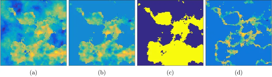
Poisson regression and LGCPs are special cases of the LSCP model. For an illustration of the exibility of the model, Figure 2 shows the log-intensity for four special cases simulated on the unit square. In these gures, all Gaussian random elds are assumed to have constant meansµ and Matérn covariance functions [37],
C(h) = σ
2
2ν−1Γ(ν)(κh)
νK ν(κh),
whereσ2 = Var(Xk(s)),κ=
√
8ν
r , andν is a smoothness parameter. Further,ris the correlation
range approximately corresponding to the value ofhwhere the correlation is0.1,Kν is a modied Bessel function of the second kind, andΓ is the Gamma function.
The patterns were generated using the same random seed such that the level set function is the same for all cases, yielding comparable results. A realization oflogλ(s)using two classes is
shown in panel (a). The log-intensity surface of the rst class has µ= 2 and r = 0.1, whereas
the second class hasµ= 0 and r= 0.2. Both elds haveσ =ν = 1. The level set eld,X0, has
a threshold value at the origin, c1 = 0, and range r = 0.4. In the gure, the regions belonging
to the two classes, and the dierence in spatial correlation range is clearly visible.
A simplication of the model is obtained by assuming that the intensity for one of the two classes is constant (change X1(s) to a constant X1, for instance). A realization of such
a log-intensity surface can be seen in Panel (b). This model might be relevant in applications where some unknown factor makes it unlikely to observe points in certain subregions and may be regarded as spatially varying zero-ination [33]. If a standard LGCP is tted to data of this type some overdispersion will be unexplained and the estimated mean eld and covariance parameters will be biased; this is not the case for the LSCP model. We discuss an example of this in Section 4. The two-class model can of course be simplied further by assuming a constant intensity for both classes, and logλ(s) is then of the form (2). This is identical to the
model of [41] and corresponds to a special case of the Random-set-generated Cox process [30]. A realization of this model is shown in Panel (c).
The last model example uses the structure of the level set formulation to capture eects on the boundary between two regions. For a model with three classes, the second class takes on the role of an interface layer between the rst and third class as can be seen in Panel (d). The log-intensity is in this case logλ(s) = P3
i=1(Xi(s) +µi(s)) Zi(s). This can be used to model
eects present on the boundary between two regions. Examples of potential applications are activity on shore lines between water and land or mixing regions between uids.
(a) (b) (c) (d)
Figure 2: Realization of the log-intensity surface, logλ(s), for the four models presented in
Section 2.2. Panel a) corresponds to the model with two random classes, Panel b) with one constant and one random, panel c) with two constant, and Panel d) is the model with two constant and a third random boundary class.
2.3 Model properties
The intensity measure Λ ={Λ(E) =R
Eλ(s)ds;E ⊆ D} for a Cox process is well-dened if λis
almost surely nite and integrable. The LSCP model with K = 1 is just the standard LGCP
model, which has a well-dened random intensity measure if realizations of the Gaussian eld are identied with their continuous modications [39]. For K > 1, a continuous modication
does not need to exist but almost sure integrability follows ifX0 is a.s. continuous which ensures
that the sets{s:ck−1<X0(s)≤ck}are a.s. Lebesgue measurable for all k∈ {1, ..., K}. Hence the LSCP model is well-dened when the realizations of all Gaussian elds are identied with their continuous modication with respect to the Lebesgue measure. By the same argument as in Theorem 3 of Møller et al. [39], ergodicity of the LSCP model follows from ergodicity oflogλ. Thus, the LSCP model is ergodic if all latent Gaussian elds are ergodic.
The following proposition gives semi-explicit formulas for the rst and second order product densities.
Proposition 2.1. For an LSCP with log-intensity (3), where{Xk}Kk=1 are zero-mean stationary
random elds with covariance functions {Ck}K
k=1, the rst moment of the intensity function
equals
ρ1(s) =E[λ(s)] =
K
X
k=1
exp
µk(s) +
Ck(0) 2
(Φ (ck−µ0(s))−Φ (ck−1−µ0(s))),
where Φ is the CDF of a standard normal distribution. Further, the second moment of λ, ρ2(s1,s2), corresponding to the second order product density equals
ρ2(s1,s2) =
K
X
k=1
exp (µk(s1) +µk(s2) +Ck(0) +Ck(|s1−s2|))pkk
+
K
X
k=1
X
l6=k
exp
µl(s1) +µk(s2) +
Ck(0) +Cl(0)
2
plk.
Here
plk= Φd(ck−µ0(s1),cl−µ0(s2))−Φd(ck−1−µ0(s1),cl−µ0(s2))
where Φd is a CDF of a standard bivariate Gaussian distribution with correlation d =
C0(|s1−s2|).
The proof is given in Appendix B. Both Φ and Φd can be evaluated using software for scientic computations. The pair-correlation function is dened asg(s1,s2) = ρ1ρ(2s(1s)1ρ,1s(2s)2), and
can hence be expressed using rst and second product densities as given in Proposition 2.1. Finally, the inhomogeneous empty space function [6, 17],F(r), for the general model is given
in the following proposition.
Proposition 2.2. For an LSCP with log-intensity (3) where Xk are zero-mean stationary ran-dom elds with covariance functions Ck, the inhomogeneous empty space function is given by
F(s0, r) = 1−E
"K Y
k=1
exp −
Z
Dk∩B(s0,r)
eµk(s)eXk(s)ds !#
,
where for a given realization of X0, Dk is the region classied ask. The proof is given in Appendix B.
2.4 Finite dimensional approximation
As for standard LGCP models, some nite dimensional approximation of the LSCP model is needed if it is to be used for inference. The discretization we use here is a classical lattice approximation. The observational domain is discretized into N subregions Di of a regular
lattice over the domain, and the point locations are replaced by counts Yi of the number of observations within each subregion Di. This yields the discretized model Yi ∼Pois(λi), where λi =
R
Djλ(s)ds and the information on the ne-scale behaviour of the point pattern behavior
is lost. The stochastic integral in the denition of λi is not Gaussian and generally dicult to handle. Therefore, a common approximation is to use λj ≈ | Dj|λ(sj), for some location (usually the center) sj ∈ Dj [39].
For any xed lattice approximation there is a positive probability that the level set eld takes values in several of the intervals{ck, ck+1}in any xed lattice cell. Since the spatial information
about the level set eld on a ner scale than the lattice discretization are lost we propose adding a nugget eect, ξj, for each lattice cell Dj. The nugget eect will model the within-cell
classication uncertainty. This gives the discretization λj ≈ | Dj|λ˜(sj), where
log ˜λ(sj) = K
X
k=1
I ck−1< X0(sj) +µ0(sj) +ξj < ck
(Xk(sj) +µk(sj)),
andξj ∼N(0, σξ2). The nugget variance,σξ2, controls the amount of mixing between the classes for a given realization of X0. This classication mechanism is equivalent to the ordered probit
model discussed in Dunlop et al. [21]. In practice, it is typically dicult to objectively discern an appropriate value forσξand hence we therefore letσξbe a regular parameter to be estimated for a xed discretization.
In Appendix A, we show consistency of this nite dimensional approximation of the likelihood for the LSCP model. More precisely, we show that the posterior distribution for the latent elds
{Xk}k computed using the lattice approximation converges, in total variation distance, to the posterior distribution of the continuous process.
3 Inference
A popular approach for Bayesian inference is through Markov chain Monte Carlo (MCMC) methodology, for instance using the Metropolis adjusted Langevin algorithm (MALA) [46] which was suggested for LGCP models by Møller et al. [39]. Another approach is through integrated nested Laplace approximation (INLA) [31, 48, 52], which when applicable can have benecial computational properties. Unfortunately the level set construction cannot be handled by INLA. In this work we propose an MCMC algorithm for tting the LSCP model and perform predictions. Specically, we propose a method based on the preconditioned Crank-Nicholson Langevin (pCNL) algorithm [16]. The algorithm is developed for the case when the target distribution (the posterior) has a Gaussian prior and a non-Gaussian likelihood, as is the case for the LSCP model. An important property of the pCNL algorithm is that it is discretization invariant [8]. This implies that as the nite dimensional approximation is made ner the mixing of the Markov Chain does not deteriorate. This is important since we utilize a rather ne discretization and thus one should expect poor mixing for an algorithm without this property, like for instance MALA.
We now present in more detail how we implement the MCMC algorithm for the LSCP model. Denote the set of parameters associated with class k asθk. For the level set eld, X0, we also
include the nugget variance, σξ, and the thresholds, {ck}k in the set θ0. By introducing an
auxiliary eldZdened such that P(Z(sj) =k) = Φ
c
k−X0(sj)
σξ
−Φck−1−X0(sj)
σξ
, we have
log ˜λ(s)=d
K
X
k=1
I(Z(s) =k) (Xk(s) +µk(s)).
This means that parameters and latent elds of dierent classes, {Xk, θk}, are conditionally independent given Z. We use this to construct a Metropolis-within-Gibbs algorithm [45] to
sample from the joint posterior. In the ith iteration of the algorithm, the following three steps are performed
1. Sample from Z|{Xk, θk}k,Y. The sampling can be performed exactly since Z(si) ⊥
Z(sj),∀i6=j given{Xk, θk}k,Y and P(Z(si) =k) is known.
2. Sample fromθk|Z,Xk using the MALA algorithm. Since parameters from dierent classes are conditionally independent, the sampling for eachθk can be performed in parallell. 3. Sample from Xk|Z, θk,Y using the pCNL algorithm. Also here, the updates for dierent
kcan be done in parallel since the elds, {Xk}Kk=0, are conditionally independent.
The computational bottleneck of the algorithm is the third step, where the latent Gaussian elds are sampled. This is computationally expensive since the spatial discretization in two dimensions will correspond to a high dimensional distribution. However, since we are using a spatial lattice discretization withN subregions, ecient sampling from the prior Gaussian eld is possible with a computational complexity of O(NlogN) using spectral methods [34] (that
4 Application
To further illustrate our approach we return to the tropical rainforest data example in Section 1 to compare the eect of considering LSCP models instead of simple Poisson regression or the LGCP model.
4.1 Data
The dataset consists of 2461 locations of trees of the species Beilschmiedia pendula in a 50
ha rectangular study plot (500 x 1000 meter) on the island of Barro Colorado in Panama,
Figure 1a. The data were acquired from the rst census of a major ongoing ecological study that started in the 1980s, designed to understand the mechanisms maintaining species richness, consisting of the observed positions of a large number of tree species ([28, 27, 13]). The study deliberately considers a spatially mapped rainforest community, arguing that population and community dynamics occur in a spatial context [26]. In addition to the spatial pattern formed by the tree locations, measurements of topographical variables and soil nutrients that potentially inuence the spatial distribution of the trees are available [32, 51, 18], with the aim of linking spatial patterns to spatial environmental variations, reected by observed topography and soil nutrients. Some of the point patterns derived from this material has been studied in, for instance, [38, 52, 31, 44] and the Beilschmiedia pendula data are available in the spatstat package [5] for the R project [1].
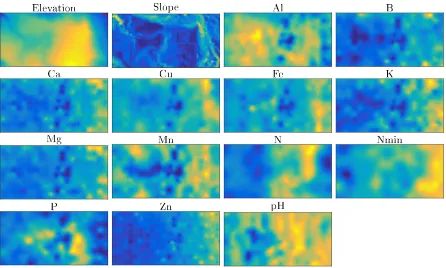
Elevation was measured and sampled on a 5x5 meter grid, and based on this an approximation of the slope at each of these grid points was calculated using a Sobel lter [54]. Soil samples were taken at 300 locations, for which the amount of 12 soil constituents (Al, B, Ca, Cu, Fe, K, Mg, Mn, N, Nmin, P, Zn) as well as the pH level were measured; these were interpolated to yield spatially continuous covariates. Since the covariates derived from the soil samples and elevation were not sampled at grid resolution they had to be interpolated to a common lattice. In this example, the model was discretized to30×60subregions over the observational window, giving
a spatial resolution of16.7×16.7 meters. The soil samples and elevation data was interpolated
to the very same resolution. The number of observed points in each subregion is shown as a two dimensional histogram in Figure 1b. The spatial interpolation of the covariates to this lattice grid was performed using bi-cubic splines with the function interp2 in Matlab (R2016a); Figure 3 shows the standardized covariates.
To avoid problems with multicollinearity among the covariates, covariates were discarded based on high variance ination factors (VIF) [42]. The covariates were discarded iteratively by rst computing the VIF for all covariates, removing the covariate corresponding to the highest VIF value if it exceeds 5 and then starting over on the new reduced set of covariates. The algorithm was stopped when none of the VIFs exceeded 5. By this procedure, the covariates B, Ca, K, and Zn were discarded, leaving 11 covariates for further analysis.
4.1.1 Models
It is obvious from Figure 1a that there is a large area in the middle of the domain where hardly any trees are growing. It is likely that some inhibitory factor prevents the trees from growing in that region. As mentioned earlier, we have anecdotal evidence that this area is covered by a swamp and that the tree species is known to be very unlikely to grow there. We test four dierent models to see how the confounding factor will aect inference., as sumarised in Table 1.
The rst is a simple Poisson regression model on the covariates, i.e. an inhomogeneous Poisson process with linear xed eects dening the log intensity as B(s)β. We will refer
Elevation Slope Al B
Ca Cu Fe K
Mg Mn N Nmin
[image:9.595.72.518.69.337.2]P Zn pH
Figure 3: The standardized covariate values on the observational domain.
to this model as the Fixed model. The second model includes a Gaussian eld to capture the variability not explained by the covariates. More precisely, we use a LGCP model with log-intensity logλ(s) = X(s) +µ(s). Here X(s) is a zero-mean Gaussian eld with Matérn
covariance with standard deviation σ and ranger andµ(s) = B(s)β.
Looking at the data, we might expect the LGCP model to explain the variation in point intensity well, except for the complete lack of observations in the central region coupled with the discontinuity in the observed intensity at the border between the large empty area and the other parts of the plot. If the habitat dependence of the trees is signicantly dierent in these two separated regions, a LSCP model with a separate class for each of the two regions might provide a better t. Therefore, the third model is a two-class LSCP model where the rst class is dened as in the LGCP model and the second class has a constant intensity xed to a low value. That is,logλ(s) = Z1(s) (X1(s) +µ1(s)) + Z2(s)C2, whereZk(s) =I(Z(s) =k). This choice of
model is tailored to partition the spatial domain in to one partition with trees and one partition with a very small probability of trees growing. Since it is hard to distinguish between dierent values of very low intensity when studying a point pattern, the low intensity class might as well be modeled with a xed intensity. We x the intensity toC2 = 0.0268, which is one tenth of the
mean intensity among the grid cells with at most1tree. We refer to this as the LGCPM model.
Finally, we consider a simplied version of this model wherelogλ(s) = Z1(s) B(s)β+ Z2(s)C2.
That is, no random eects in any of the two classes. This will be referred to as the FixedM model.
FIXED: logλ(s) = B(s)β
LGCP: logλ(s) = X(s) + B(s)β
LGCPM: logλ(s) = Z1(s) (X(s) + B(s)β) + Z2(s)C2
FIXEDM: logλ(s) = Z1(s) B(s)β+ Z2(s)C2
[image:9.595.159.438.659.715.2]The posterior distributions of the parameters and latent elds were estimated using the proposed MCMC method of Section 3. In order to reduce boundary eects, the lattice was extended by 350 m for the level set eld and by 220 m for the latent Gaussian elds of the
classes (implicitly assuming correlation ranges smaller than350 m for classication and 220m
within classes). The smoothness parameters of the Gaussian elds were xed at ν = 1 and
the following independent prior distributions for the model parameters (when applicable) were used: i)N(0,10)-priors for the xed eects; ii)N(0,4)-priors for the threshold parameters; iii) an
exponential prior with mean 2, Exp(2)forσkexcept thatσ0= 1is xed due to the identiability
issues discussed in Section 2.1; iv) Exp(200)-priors truncated from below at the lattice distance
and from above at the lattice extension range forrk; this ensures that no wrap-around artifacts
were introduced and that the correlation range was not smaller than the discretization distance; v) an Exp(0.1)prior truncated from above at1for the nugget standard deviation; this yields an
expected a priori standard deviation of approximately0.1and ensures that the nugget variance
does not dominate the spatial dependency in the level set eld.
The standard deviations of the Gaussian elds were given exponential priors in order to penalize model complexity, following the PC prior framework of [55, 53]. This corresponds to penalization of the Gaussian elds, {Xk}Kk=1, when the covariates alone can explain the
variation. The range parameters were given exponential priors using similar reasoning to the standard deviations where no spatial dependency corresponds to the base model. However, the distribution was truncated since no information exists on ranges below the lattice diameter due to the spatial discretization. The covariates were standardized to mean0and variance1. Hence,
the xed eects prior yields a penalisation from the base model of no xed eects. The nugget for the level set eld was considered as a deviation from the base model (without a nugget) and hence penalised by an exponential distribution. The MCMC chains were run for 5·106
iterations on a standard contemporary laptop. The simulations took 2.3 hours for the Fixed
model, 11 hours for the LGCP model, 32 hours for the LGCPM model, and 24 hours for the
FixedM model.
4.1.2 Model validation
To validate the models we use a standard approach from point process literature [38, 30, 4] that compares a summary characteristic estimated from the observed point pattern with envelopes based on the summary characteristics estimated for point patterns simulated using the tted models. As a summary characteristic we choose the pair correlation function [30] which is a second order functional summary characteristic characterizing the expected number of points at distances close to r from an observed point.
The pair correlation function with isotropic edge correction was estimated using the function pcf from the spatstat package [5]. An estimate from the observed data as well as estimates for each out of 5000 point pattern realizations was acquired for each model. Here we have rst
looked at point pattern realizations based on5000draws of parameter values (θ0,θ1,. . .) from
the posterior distribution given the observed data. That is, we compare the four models with parameter values that are reasonable given the observed trees data. Secondly we have also looked at5000point pattern realizations, each one sampled from an anisotropic Poisson process
with an intensity function drawn from the posterior distribution conditioned on the observed data for each of the four models. That is, comparing point patterns generated from the posterior distributions of each of the four models. The draws from the posterior distributions were acquired using the MCMC simulations.
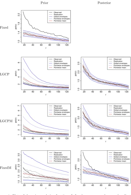
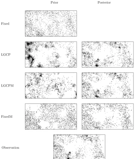
The pair correlation function for the observed point pattern as well as 5 randomly chosen realizations can be seen in Figure 4. The pointwise mean among all realizations and the90%
velopes (both global and pointwise) have been plotted in the gure. The left column corresponds to realizations from the prior models using parameter values from the posterior distributions. The right column corresponds to realizations from the posterior point processes. For the Fixed model, the prior and posterior model do not dier since no random eects are present. Hence, only one gure is present in the corresponding column.
In general, the plots in the left hand (LH) column in Figure 4 reect how well the simulated patterns resemble the overall pattern structure in the original data, and the plots on the right hand (RH) side how well the simulated patterns resemble the original pattern itself. The pair correlation function is dened for stationary patterns. In the current context, where we want to assess the models' ability to capture non-smooth non-stationarity in the pattern, the values of the summary characteristic might not be able to indicate issues with this type of structure. Hence, we also consider some randomly chosen examples of the corresponding simulated point patterns for each of the same scenarios as in Figure 4; these are shown in Figure 5. To assess the models' performance we consider these two gures together.
For the simplest model, the Fixed model, the estimated pcf for the observed point pattern is above the envelopes for all distances (Figure 4). This clearly indicates that the model that is based on covariates only does not suciently capture aggregation at any spatial scale and is clearly inappropriate for this data set. This is not surprising since it had been anticipated that the covariates are unable to reect the spatial structure resulting from the presence/absence of the swamp. In addition, they might also not be sucient to capture small scale clustering, resulting from dispersal limitation. The relevant simulated pattern in Figure 5 reects this very clearly; the pattern does not show any of the small scale clustering that's evident in the observed pattern and it does not suciently explain the large empty area where the swamp is located. There is an area with lower point intensity, perhaps a result of some of the covariates being correlated with the presence of the swamp.
For the standard LGCP model, the estimated pair correlation functions in Figure 4 (LH and RH) for the observed point pattern remain inside the global envelopes. However, for small distances, the mean function for the patterns simulated from the tted model is above the function for the observed pattern in the LH plot. This is reected in the low values of the black line relative to the red line for up to about 40 meters radius r. This indicates that the model accounts for less clustering at small distances than has been observed in the pattern formed by the rainforest trees. This is likely a result of the model attempting to average the parameters for the Gaussian eld across the whole plot; the Gaussian eld in the model attempts to explain spatial structures that the covariates cannot explain in general as well as the the eect of the swamp. This is also evident in the relevant LH plot in Figure 5. The pattern shows some empty areas, perhaps smaller than the swamp, but this is hard to discern from a single pattern only. It also shows local clustering which is much stronger than in the original pattern. The associated RH plot looks rather similar to the observed pattern with perhaps too many points in the clustered areas.
For the LGCPM model, the mean line and the estimated line pair correlation functions are very similar, even though the red line is slightly above the black line for small distances in the LH plot of Figure 4. This might indicate that slightly more local clustering is reected in the model than is exhibited by the actual pattern. The general spatial structure in the LH simulated pattern appears to be much more similar to the general structure in the original pattern than that simulated from the LGCP model, neither overly exaggerating the clustering nor the emptiness. The RH equivalent again strongly resembles the original pattern, perhaps with slightly too many points in the areas with local clustering as indicated by the pair correlation function.
Prior Posterior
Fixed
20 40 60 80 100 120
1.0 1.4 1.8 2.2 r pcf(r) Observed Realization Global envelopes Pointwise envelopes Pointwise mean LGCP
20 40 60 80 100 120
2 4 6 8 r pcf(r) Observed Realization Global envelopes Pointwise envelopes Pointwise mean
20 40 60 80 100 120
1.0 1.5 2.0 2.5 r pcf(r) Observed Realization Global envelopes Pointwise envelopes Pointwise mean LGCPM
20 40 60 80 100 120
1 2 3 4 5 6 7 r pcf(r) Observed Realization Global envelopes Pointwise envelopes Pointwise mean
20 40 60 80 100 120
1.0 1.5 2.0 2.5 r pcf(r) Observed Realization Global envelopes Pointwise envelopes Pointwise mean FixedM
20 40 60 80 100 120
1.0 1.5 2.0 2.5 3.0 3.5 r pcf(r) Observed Realization Global envelopes Pointwise envelopes Pointwise mean
20 40 60 80 100 120
[image:12.595.82.505.67.696.2]1.2 1.6 2.0 r pcf(r) Observed Realization Global envelopes Pointwise envelopes Pointwise mean
Figure 4: Plots of the pair correlation function. Left column uses envelopes and realizations from point patterns generated using the prior model with parameters drawn from the posterior distribution. Right column uses envelopes and realizations drawn from the posterior point processes. Each panel show the value for the observed point pattern (black), 5 randomly chosen realizations (gray), the pointwise mean (red), 90% pointwise (blue dotted) and global (blue)
Prior Posterior
Fixed
LGCP
LGCPM
FixedM
[image:13.595.76.514.114.631.2]Observation
σξ
Fixed LGCP LGCPM FixedM
0 0.2 0.4 0.6 0.8
r0
Fixed LGCP LGCPM FixedM 0
100 200 300 400
c1
Fixed LGCP LGCPM FixedM
-1 0 1 2
σ1
Fixed LGCP LGCPM FixedM 0
0.5 1 1.5
2 r1
Fixed LGCP LGCPM FixedM 0
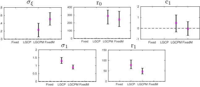
[image:14.595.137.461.71.213.2]50 100 150
Figure 6: The mean (cross) and 95% credible intervals (lines) for the eld parameters.
in the RH plot of Figure 4, where the function estimated for the observed pattern is above the envelopes up to a distance of about 40 meters, but is also evident in the associated LH plot. The simulated patterns in Figure 5 tell a similar story; the swamp is reasonably well accounted for but there is a clear lack of local overdispersion in the patterns.
4.1.3 Analysis of covariates and spatial structure
The models discussed here, relating a spatial pattern to spatially continuous covariates may be of interest for a number of reasons. Commonly, one seeks to understand habitat preferences of a particular species as reected in the relationship between the point pattern and the covariates. In addition, it might be of interest to understand the nature of the spatial structure that remains unexplained by the covariates.
To investigate the spatial structure, we rst look at the mean value and95%credible intervals
for the random eld parameters of the models. These are presented in Figure 6. Observing the dierence between r1, and σ1 values of the LGCP and LGCPM models show how the empty
region will aect the estimation of the spatial dependency structure. Here, the LGCPM model shows a signicantly lower variance and clearly lower correlation range. This is natural since the Gaussian eld for the LGCPM model does not need to explain both the eect of natural spatial dependency between growth of trees as well as the unknown inhibitory eect that causes trees to not grow at all in certain regions of the forest. And nally we note that σ has a large eect (signal to noise ratio equals 1
σ) indicating that the Matérn eld forX0 cannot explain the
classication on its own. This is clearer for the FixedM model, where classication jumps more sporadically between adjacent grid cells due to the over-simplied structure of the classes.
In Figure 7 the mean posterior log intensities,{logλi}N
i=1are presented as kriging predictions
for each of the four models. The gure also shows the posterior probabilities P(Z(s) = 2|Y),
giving an indication of the region with very few trees. The posterior log intensity surface of the LGCPM shows sharp boundaries contrary to the smoothly varying in the LGCP. The classication in the FixedM model is more noisy than that of the LGCPM model and a larger proportion of the observation window is classied as being the empty region. Once again, this is connected to the larger value ofσξ and caused by the FixedM having to explain the intensity with a much simpler model.
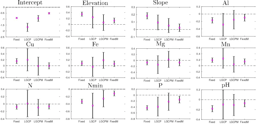
The relationship between the tree intensity and the covariates is also of interest, and in practice is often the focus of a study. Recall that 12 covariates of the original 16 covariates are considered here; 11 true covariates and one intercept term. Figure 8 shows the mean and 95%
credible intervals for each of these covariates for all models. The rst question is which of the covariates have a signicant impact on the spatial distribution of the trees and hence reect a
(a) Fixed (b) LGCP
(c) LGCPM (d) FixedM -2
-1 0 1 2 3 4
(e) LGCPM
(f) FixedM 0
[image:15.595.77.520.75.244.2]0.1 0.2 0.3 0.4 0.5 0.6 0.7 0.8 0.9 1
Figure 7: Mean posterior log intensity surface, λ (left) and mean classication for the models where applicable (right)
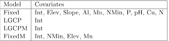
Model Covariates
Fixed Int, Elev, Slope, Al, Mn, NMin, P, pH, Cu, N
LGCP Int
LGCPM Int
FixedM Int, NMin, Elev, Mn
Table 2: Signicant covariates on a 5% level for the covariates using Holm-Bonferroni correction to correct for multiple hypothesis tests.
habitat preference of the species. To answer this we asses which of the regression coecients in
β that are signicantly dierent from zero. Empirical p-values are computed from the sampled
posterior distributions. Since there are 12 xed eects, the p-values were adjusted using Holm-Bonferroni correction [25] to account for multiple testing. Table 2 shows the covariates that were considered signicant, at a signicance level of5%, for each of the four models.
The FixedM model identies a smaller number of signicant covariates than the Fixed model. This is not surprising since the covariates do not need to explain the lack of trees in the empty domain anymore. It should be noted that we found that the Fixed and FixedM models did not t the data, see Figure 4. Hence, nding signicant covariates could be due to model misspecication rather than an actual relationship with the observed point pattern. For the LGCP and LGCPM models, only the intercepts are signicant.
5 Discussion
We have considered the problem of Bayesian level set inversion for point process data. The proposed model can be seen as a generalization of the LGCP model where the latent Gaussian eld is extended to a level set mixture of Gaussian elds. We derived basic model properties and in Appendix A showed consistency of the posterior probability measure of nite-dimensional ap-proximations to the continuous model. A computationally ecient MCMC method for Bayesian inference, based on the preconditioned Crank-Nicholson Langevin algorithm, was presented. A topic of further research could be to investigate other, potentially even quicker, estimation methods such as based on INLA in combination with variational Bayes.
[image:15.595.157.441.296.366.2]Intercept
Fixed LGCP LGCPM FixedM -2.5 -2 -1.5 -1 -0.5 0 Elevation
Fixed LGCP LGCPM FixedM
-0.4 -0.2 0 0.2 0.4 0.6 Slope
Fixed LGCP LGCPM FixedM -0.1
0 0.1 0.2
0.3 Al
Fixed LGCP LGCPM FixedM
-0.6 -0.4 -0.2 0 0.2 Cu
Fixed LGCP LGCPM FixedM
-0.4 -0.2 0 0.2 0.4 0.6 Fe
Fixed LGCP LGCPM FixedM
-0.4 -0.2 0 0.2 0.4 0.6 Mg
Fixed LGCP LGCPM FixedM
-0.6 -0.4 -0.2 0 0.2 0.4 Mn
Fixed LGCP LGCPM FixedM
-0.4 -0.2 0 0.2 0.4 0.6 N
Fixed LGCP LGCPM FixedM
-0.4 -0.2 0 0.2
0.4 Nmin
Fixed LGCP LGCPM FixedM
-0.8 -0.6 -0.4 -0.2
0 P
Fixed LGCP LGCPM FixedM
-0.8 -0.6 -0.4 -0.2 0 0.2 pH
Fixed LGCP LGCPM FixedM
[image:16.595.78.519.72.288.2]-0.4 -0.2 0 0.2
Figure 8: The mean (cross) and 95% credible intervals (lines) for the posterior marginal distri-bution of xed eect for the four dierent models.
rainforest. The example was relevant in the current context since the point pattern shows clear signs of being aected by some confounding factor (mainly reecting the presence or absence of a swamp). Soil and topography covariates are at most slightly correlated with the swamp and hence cannot explain the nearly complete absence of points in that area. A standard LGCP model accounts for remaining spatial structures through a single smooth Gaussian eld. The LSCP model we propose here can have a level set mixture of two Gaussian elds, one component explaining local spatial structures (such as those resulting from dispersal limitation) and another constant component explaining the absence or presence of the emptiness.
We tted 4 dierent models to the data, which all could be viewed as special cases of the LSCP models, a simple model with only covariates (Fixed), a standard LGCP process model, a LSCP model with one constant class and one class modeled using a Gaussian eld (LGCPM) and a simplied version of this which only had xed eects in the rst class (FixedM). We compared the performance of the four models using simulations from the tted models to the observed data, both based on summary characteristics from repeated simulation and by visually comparing the resulting spatial structures in the simulated patterns to those in the observed pattern. The dierences in model performance were most evident in the visual comparison of the generated patterns. The LGCPM clearly reproduced the original pattern structure better than the other models, with the Fixed model neither showing local clustering nor a meaningful empty area, the LGCP model exhibiting exaggerated local clustering and the FixedM model not accounting for local clustering. The pair correlation function reected these features as well, but not in as an obvious way. The analysis of the tropical rainforest showed that inference on both the Gaussian eld parameters and covariates were aected by allowing for a second class in the model. It suggests that the inference drawn based on the LGCP model were biased by the confounding factor and that no covariates can be considered statistically signicant.
Patterns simulated from the model might also be useful for aiding the interpretation and understanding of underlying ecological mechanisms. For instance, simulating patterns based on the parameters estimated from the LGCPM but not involving the component relating to the swamp in the simulation as it is clear that it leads to low point intensities would provide an insight into what spatial structures looked like if the swamp was not present. This is interesting,
as the swamp eect trivially leads to spatial structures that are uninteresting but very obvious on visual inspection.
Future analysis could consider using xed eects also with the level set eld, X0, in order
to investigate which covariates explain the classication, a feature of the proposed model that we have not yet investigated. Further, multi-type point patterns may also be analyzed with the proposed model class for instance for the joint analysis of several species of plants. This could be performed by introducing multivariate Gaussian random elds for the classes, i.e. for{Xk}Kk=1.
Another possibility is letting several species share the same level set eld,X0, or classications
eld, Z, but use independent class elds,{Xk}Kk=1. In this way, information about X0 could be
pooled from several point patterns jointly.
Furthermore, the approach may also be relevant in larger scale studies, for example in the context of species distribution modelling, where data collection eort varies in space and whole spatial areas have not been surveyed or only very few surveys have taken place, despite providing potentially suitable habitat for a species. This would create large areas relatively empty of points for which spatial covariates are available. In particular, if suitable covariates were available that might be linked to survey eort, such as population density or accessibility, a suitable level set mixture model could account for this.
A problem with the spectral approach used in this work is that the spatial discretization has to be on a lattice. In applications where such restrictions are problematic, the sampling of the Gaussian elds could be performed with a dierent method. Generally this requires
(KN3) operations. A possible approach to remedy this would be to acquire a Gaussian Markov
random eld approximation of the problem. This idea has been studied by [35, 47, 52] revealing computationally attractive properties on arbitrary domains. An adaptation of the method by Simpson et al. [52] to the LSCP model would reduce the computational cost toO(KN3/2)while
still allowing for arbitrary spatial discretizations.
Another issues that needs further investigation relates to the prior choice for the parameters of the Gaussian random eld as these can substantially inuence the smoothness and, as a result, the signicance of the spatial covariates. A spatial eld that is too wiggly can easily lead to overtting, rendering any covariates insignicant, while a eld that is too smooth dees its very purpose. Some work has been done on investigating this in the context of pc priors for log Gaussian Cox processes [55], but there is room for further investigation.
6 Acknowledgements
The authors gratefully acknowledge the nancial support from the Knut and Alice Wallenberg Foundation, the Swedish Research Council Grant 2016-04187, and the ÅForsk foundation. We would like to thank the people at the Center of tropical forest research, Smithsonian Tropical Research Institute for the extensive forest census plot and for making the data publicly available. The BCI forest dynamics research project was founded by S.P. Hubbell and R.B. Foster and is now managed by R. Condit, S. Lao, and R. Perez under the Center for Tropical Forest Science and the Smithsonian Tropical Research in Panama. Numerous organizations have provided funding, principally the U.S. National Science Foundation, and hundreds of eld workers have contributed.
References
[1] The R Project for Statistical Computing. URL https://www.r-project.org/.
[2] R.J. Adler and J.E. Taylor. Random Fields and Geometry. Springer, 2007. ISBN 978-0-387-48112-8.
[3] J-M. Azaïs and M. Wschebor. Level Sets and Extrema of Random Processes and Fields. Wiley, 1 edition, 2009. ISBN 04704093393.
[4] A. Baddeley, E. Rubak, and R. Turner. Spatial point patterns: methodology and applications with R. CRC Press, 2015.
[5] Adrian Baddeley, Ege Rubak, and Rolf Turner. Spatial Point Patterns: Methodology and Applications with R. Chapman and Hall/CRC Press, London, 2015. URL http://www. crcpress.com/Spatial-Point-Patterns-Methodology-and-Applications-with-R/ Baddeley-Rubak-Turner/9781482210200/.
[6] A.J. Baddeley. Non- and semi-parametric estimation of interaction in inhomogeneuous point patterns. Statistica Neerlandica, 54(3):329350, 2000.
[7] S. Barman and D. Bolin. A three-dimensional statistical model for imaged microstructures of porous polymer lms. Journal of Microscopy, 269(3):247258, 2018.
[8] Alexandros Beskos, Gareth Roberts, Andrew M Stuart, and Jochen Voss. MCMC methods for diusion bridges. Stochastics and Dynamics, 8(3):319350, 2008.
[9] M. Burger. A level set method for inverse problems. Inverse problems, 17(5):13271355, 2001.
[10] D. F. R. P. Burslem, N. C. Garwood, and S. C. Thomas. Tropical forest diversity the plot thickens. Science, 291:606607, 2001.
[11] E.T. Chung. Electrical impedance tomography using level set representation and total variational regularization. Journal of computational physics, 205:357372, 2005.
[12] R. Condit. Tropical Forest Census Plots. Springer-Verlag and R. G. Landes Company, Berlin, Germany, and Georgetown, Texas., 1998.
[13] R. Condit. Tropical Forest Census Plots: Methods and Results from Barro Colorado Island, Panama and a Comparison with Other Plots. Springer Berlin Heidelberg, 1998. ISBN 9783662036648.
[14] R. Condit, P. S. Ashton, P. Baker, S. Bunyavejchewin, S. Gunatilleke, N. Gunatilleke, S.P. Hubbell, R.B. Foster, A. Itoh, J.V. LaFrankie, H.S. Lee, E. Losos, N. Manokaran, R. Sukumar, and T. Yamakura. Spatial patterns in the distribution of tropical tree species. Science, 288:14141418, 2000.
[15] S.L. Cotter, M. Dashti, and A.M. Stuart. Approximation of Bayesian inverse problems for PDEs. SIAM journal on numerical analysis, 48(1):322345, 2010.
[16] S.L. Cotter, G.O. Roberts, A.M. Stuart, and D. White. MCMC Methods for Functions: Modifying Old Algorithms to Make Them Faster. Statistical Science, 28(3):424446, 2013. [17] D.J. Daley and D. Vere-Jones. An Introduction to the Theory of Point Processes: Volume
II: General Theory and Structure, volume 2. Springer, 2003. ISBN 0-387-95541-0.
[18] J. Dalling, R. John, K. Harms, R. Stallard, and J. Yavitt. Soil Maps of Barro Col-orado Island 50 ha Plot. URL "http://ctfs.si.edu/webatlas/datasets/bci/soilmaps/ BCIsoil.html".
[19] O. Desjardins and H. Pitsch. A spectrally rened interface approach for simulating multi-phase ows. Journal of computational physics, 228(5):16581677, 2009.
[20] P.J. Diggle. Statistical Analysis of Spatial and Spatio-Temporal Point Patterns. Third edition edition, 2014.
[21] M.M. Dunlop, M.A. Iglesias, and A.M. Stuart. Hierarchical Bayesian level set inversion. Statistics and Computing, pages 130, 2016.
[22] M. Fuentes. A new class of nonstationary spatial models. Unpublished manuscript, available at http://www.stat.unc.edu/postscript/rs/nonstat.pdf, 2001.
[23] J. Hendrix, T. Dekens, W. Schrimpf, and D.C. Lamb. Arbitrary-Region Raster Image Correlation Spectroscopy. Biophysical Journal, 111(8):17851796, 2016.
[24] M.D. Higgs and J.A. Hoeting. A clipped latent variable model for spatially correlated ordered categorical data. Computational statistics and data analysis, 54:19992011, 2010. [25] S. Holm. A Simple Sequentially Rejective Multiple Test Procedure. Scandinavian journal
of statistics, 6(2):6570, 1979.
[26] S. P. Hubbell. The Unied Neutral Theory of Biodiversity and Biogeography. Monographs in Population Biology 32, Princeton University Press, 2001.
[27] S. P. Hubbell, R. B. Foster, S. T. O'Brien, K. E. Harms, R. Condit, B. Wechsler, S. J. Wright, and S. Loo de Lao. Light-Gap Disturbances, Recruitment Limitation, and Tree Diversity in a Neotropical Forest. Science, 283(5401):554557, 1999.
[28] S. P. Hubbell, R. Condit, and R. B. Foster. Barro Colorado Forest Census Plot Data, 2005. URL http://ctfs.si/edu/datasets/bci.
[29] M.A. Iglesias, Y. Lu, and A.M. Stuart. A Bayesian level set method for geometric inverse problems. Interfaces and free boundaries, 18(2):181217, 2016.
[30] J. B. Illian, A. Penttinen, H. Stoyan, and D. Stoyan. Statistical Analysis and Modelling of Spatial Point Patterns, volume 70. John Wiley & Sons, 2008.
[31] J.B. Illian, S.H. Sørbye, and H. Rue. A toolbox for tting complex spatial point process models using integrated nested Laplace approximation. The Annals of Applied Statistics, 6 (4):14991530, 2012.
[32] R. C. John, J. W. Dalling, K. E. Harms, J. B. Yavitt, R. F. Stallard, M. Mirabello, S. P. Hubbell, R. Valencia, H. Navarrete, M. Vallejo, and R. B. Foster. Soil nutrients inuence spatial distributions of tropical tree species. Proceedings of the National Academy of Sciences USA, 104:864869, 2007.
[33] D. Lambert. Zero-Inated Poisson Regression, With an Application to Defects in Manu-facturing. Technometrics, 34(1):114, 1992.
[35] F. Lindgren, H. Rue, and J. Lindström. An explicit link between Gaussian elds and Gaus-sian Markov random elds: the stochastic partial dierential equation approach. Journal of the Royal Statistical Society, 73(4):423498, 2011.
[36] R.J. Lorentzen, G. Naevdal, and A. Shaeirad. Estimating Facies Fields by Use of the En-semble Kalman Filter and Distance Functions - Applied to Shallow-Marine Environments. SPE Journal, 3(1):146158, 2012.
[37] B. Matérn. Spatial Variations, volume 36. Springer-Verlag, 1986. ISBN 9780387963655. [38] J Møller and R.P. Waagepetersen. Modern Statistics for Spatial Point Processes.
Scandi-navian Journal of Statistics, 34(4):643684, 2007.
[39] J Møller, A.R. Syversveen, and R.P. Waagepetersen. Log Gaussian Cox Processes. Scandi-navian journal of statistics, 25(3):451482, 1998.
[40] V.V. Mourzenko. Percolation in two-scale porous media. The European physical journal B, 19(1):7585, 2001.
[41] M. Myllymäki and A. Penttinen. Bayesian inference for Gaussian excursion set generated Cox processes with set-marking. Statistics and computing, 20(3):305315, 2010.
[42] J. Neter, W. Wasserman, and M.H. Kutner. Applied Linear Regression Models. Irwin, second edition edition, 1989. ISBN 0-256-07068-7.
[43] D.B. Owen. A table of normal integrals. Communication in Statistics - Simulations and Computation, 9(4):389419, 1980.
[44] T. Rajala and J. Illian. A family of spatial biodiversity measures based on graphs. Envi-ronmental and ecological statistics, 19(4):545572, 2012.
[45] C.P. Robert and G. Casella. Monte Carlo statistical methods. Springer, 2 edition, 2004. ISBN 9781475741452.
[46] G.O. Roberts and R.L. Tweedie. Exponential convergence of Langevin distributions and their discrete approximations. Bernoulli, 2(4):341363, 1996.
[47] H. Rue and L. Held. Gaussian Markov random elds, volume 104. Chapman and Hall, 2005. ISBN 0203492021.
[48] H. Rue, S. Martino, and N. Chopin. Approximate Bayesian inference for latent Gaussian models by using integrated nested Laplace approximations. Journal of the royal statistical society: series B, 71(2):319392, 2009.
[49] F. Santosa. A level-set approach for inverse problems involving obstacles. ESAIM: Control, Optimisation and caculus of variations, 1:1733, 1996.
[50] B. Scheuermann and B. Rosenhahn. Analysis of Numerical Methods for Level Set Based Image Segmentation. Lecture notes in computer science, 5876(2):196207, 2009.
[51] L. A. Schreeg, W. J. Kress, D. L. Erickson, and N. G. Swenson. Phylogenetic analysis of local-scale tree soil associations in a lowland moist tropical forest. PLoS ONE, 5:110, 2010. [52] D. Simpson, J.B. Illian, F. Lindgren, S.H. Sørbye, and H. Rue. Going o grid: computational
ecient inference for log-Gaussian Cox processes. Biometrika, 103(1):4970, 2016.
[53] D. Simpson, H. Rue, A. Riebler, T.G. Martins, and Sørbye S.H. Penalising Model Com-ponent Complexity: A Principled, Practical Approach to Constructing Priors. Statistical science, 32(1):128, 2017.
[54] M Sonka, V Hlavac, and R Boyle. Image Processing, Analysis, and Machine Vision, chapter Image pre-processing. Thomson, 2008.
[55] S. H. Sørbye, J. B. Illian, D. P. Simpson, D. Burslem, and H. Rue. Careful prior spec-ication avoids incautious inference for log-gaussian cox point processes. arXiv preprint arXiv:1709.06781, 2017.
[56] A.M. Stuart. Inverse problems: A Bayesian perspective. Acta numerica, 19:451559, 2010.
A Theoretical results
In this section, we will theoretically justify the two approximations of the LSCP process that are needed for inference. The rst is the nite dimensional approximation from Section 2.4 and the second is the truncation needed for the fast Fourier transform in Section 3.
Fork={0, ..., K}, letXkbe a Gaussian random eld on the spatial domainD= [0,1]d⊂Rd,
dened on a complete probability space. We will show the results using methods similar to those in [15, 29, 52] and for this it is convenient to represent the elds as Gaussian measuresµ(0k). To simplify the presentation, we will assume a specic covariance operator,C, related to the Matérn
covariance function. However, the results can be extended to more general densely-dened, self-adjoint, positive denite operators and to more general bounded domains.
Let µ(0k) = N(0,C), where C = τ2A−α with A = κ2 −∆. Here τ, κ2 and α are positive parameters and A : D(A) ⊂ L2(D) → L2(D), here D(A) denotes the domain of A. Further
we impose periodic boundary conditions. Denote the eigenvalues of A as {λj}j∈N , which are
arranged in a nondecreasing order, and the corresponding eigenfunctions as{ej}j∈N, which form
a complete orthonormal basis for L2(D). The fractional power operatorAα :D(Aα) → L2(D)
is dened by
Aαu=X
j∈N
λαj hu, ejiej.
For any α, the subspaceHα :=D(Aα/2) is a Hilbert space
Hα={u:X
j∈N
λαj| hu, eji |2 <∞},
with respect to the inner product hφ, ψiα =
Aα/2φ, Aα/2ψ
and corresponding norm kφkα = P
j∈Nλ
α j hφ, eji
2.
With this choice of covariance operator, we have that if u ∼µk0, then u ∈ Hs for any s < α−d/2µk0-almost surely [21, Theorem 1]. Furthermore,uis almost surely p-times dierentiable if α−d/2> p. We will need this dierentiability and we formulate it as an assumption. Assumption A.1. The classication eld X0 is almost surely a Morse function with strictly
positive variance at all locations in the domain, and fork >0the Gaussian eldsXk are almost surely dierentiable.
The dierentiability assumption is satised by assuming α > 2. The Morse function
a theorem equivalent to the Sobolev embedding theorem for our Hs space [56, Theorem 2.10]. That is, kXkkL∞ ≤ CkXkks if Xk ∈ Hs and s > d/2. For our case with periodic boundary
conditions the spaceHs is even equivalent to the Sobolev space Hs. We thus have thatXkis represented as a Gaussian measure,µ
(k)
0 , onHαand we can choose an
appropriate σ-algebra such as the probability space(Hα,Σk, µ(k)
0 )becomes complete (see [29]).
Likewise X = {X}K
k=0 can be represented by a product measure µ0 on the complete measure
space X = (Ω,Σ, µ0), where Ω is the product space of each Hα and Σ is the corresponding
productσ-algebra.
Since the LSCP model denes the point process as a non-homogeneous Poisson process conditioned on X, the likelihood potentials for the continuous and nite dimensional models,
dened in Section 2.4, are
Φ(X; Y) = Z
D
λ(s; X)ds− X sj∈Y
logλ(sj; X), (4)
ΦN(X; Y) =X
i∈N
(| Di|λ(˜si; X)−Yilogλ(˜si; X)). (5)
Here, N is the number of discretized regions in the lattice approximation and Yi denotes the number of observations in Di. Further, s˜i is the midpoint of each Di, and sj is the location of the jth point in the point pattern Y. Based on these likelihoods, we can now dene the
corresponding posterior measures as follows.
Proposition A.2. If Assumption A.1 holds, we can dene posterior measures using Radon-Nikodym derivative with respect toµ0:
dµ dµ0
(X) = 1
Cµ(Y)
exp (−Φ(X; Y)),
dµN dµ0
(X) = 1
CµN(Y)
exp −ΦN(X; Y)
,
(6)
where Cµ(Y) and CµN(Y) are normalizing constants.
The proof is given in Appendix B. Since only the discretized model can be used for inference, it is important to know that the approximation µN converges to the true posterior, µ, as the discretization becomes ner. The following theorem shows that this indeed is the case with respect to the total variation distance, dTV(µ, µN) = 2 supE∈FX |µ(E)−µ
N(E)|.
Theorem A.3. Let Assumption A.1 hold and let µN and µ be the posterior measures dened in (6). ThendTV(µ, µN)→0 asN → ∞.
The proof is given in Appendix B. Also the latent elds,X, need to be approximated by nite
dimensional representations for inference. We will do this by truncating the basis expansion of the eld top terms:
X≈X˜ =
p
X
j=1
ξjλαjej,
where ξj are independent standard normal variables. We will refer to the model using a dis-cretization of the observational domain and nite dimensional approximations ofX as the fully
discretized model. The advantage with using this truncation is that we can use the fast Fourier transform for simulating the eld. To show that we still have convergence under this approxi-mations, note that the nite dimensional approximation of X can be viewed as an orthogonal
projection ofXon to the space spanned by the eigenfunctions{ej}j≤p as is done in Cotter et al. [15]. We dene the projection operator Pp such that X(˜ s) = PpX(s). It is now possible to dene a posterior probability measure forµ˜N by it's Radon-Nikodym derivative as
dµ˜N
dµ0
(X) = 1
Cµ˜N(Y)
exp −ΦN(PpX; Y). (7)
An important consequence of this denition is that the posterior measure is absolutely continuous with respect toµ0 and measurable with respect toΣ. The interpretation of µ˜N is that the data
will only aect the projection,PpX. We can now show that also under this approximation, we
get convergence to the true posterior.
Theorem A.4. Let the measure µ˜N be dened by (7), and let the measureµ be dened by (6). If µ0 satises Assumption A.1, thendTV(µ,µ˜N)→0 asN → ∞ andp→ ∞.
The proof is given in Appendix B.
B Proofs
Proof of Proposition 2.1. For the rst moment, note that
E[λ(s)] =E[exp(X(s))]
=
K
X
k=1
E[exp(Xk(s) +µk(s))|X0(s) +µ0(s)∈(ck−1, ck]]P(X0(s) +µ0(s)∈(ck−1, ck])
=
K
X
k=1
E[exp(Xk(s) +µk(s))]P(X0(s) +µ0(s)∈(ck−1, ck])
=
K
X
k=1
exp
µk(s) +
Ck(0) 2
P(X0(s) +µ0(s)∈(ck−1, ck]),
where the nal equality follows from the explicit form of the expectation of a log-normal random variable.
The second moment follows by similar calculations when considering that both points in space can be part of one of the K classes. Using the covariance of a bivariate log-normal distribution and dening
plk:=P(X0(s1) +µ0(s1)∈(ck−1,ck]∩X0(s2) +µ0(s2)∈(cl−1,cl])
= Z ck
ck−1
Φ
cl−µ∗(u) σ∗(u)
−Φ
cl−1−µ∗(u)
σ∗(u)
e−
(u−µ0(s1))2 2C0(0) √
2π du,
where µ∗(u) =µ0(s2) +
C0(|s1−s2|)
C0(0) (u−µ0(s1)) is the conditional expectation ofX0(s2) +
µ0(s2)|X0(s1) +µ0(s1) =uandσ∗(u) =
q
C0(0)−C0(|s1−s2|)
2
C0(0) is the corresponding conditional
Remember that C0(0) = 1 to make the model identiable with respect to the threshold
parameters. plk can then be dened through
Z ck
−∞
Φ
cl−µ∗(u) σ∗(u)
e−(u−µ0(s1))
2
2 √
2π du
= Z ck
−∞
Φ
cl−µ0(s2)
σ∗(u) +µ0(s1)
C0(|s1−s2|)
σ∗(u) −u
C0(|s1−s2|)
σ∗(u)
ψ(u−µ0(s1))du
= Z ck
−∞
Φ (a+ub)ψ(u−µ0(s1))du=
Z ck−µ0(s1) −∞
Φ (a+bµ0(s1) +yb)ψ(y)dy,
where the variable substitution,y=u−µ0(s1), was used. Here,a= cl−σ∗µ(0u()s2)+µ0(s1)C0(|σs∗1(−u)s2|),
and b=−C0(|s1−s2|)
σ∗(u) . Using10,010.1from [43] then yields
Z ck−µ0(s1) −∞
Φ (a+bµ0(s1) +yb)ψ(y)dy=
1
2π√1−d2
Z ck−µ0(s1) ∞
Z a+√bµ0(s1)
1+b2
∞
e−
x2+y2−2xyd
2(1−d2) dxdy,
whered= √−b
1+b2. Finally, 1 +b
2 = 1 +C0(|s1−s2|)2
σ∗(u)2 = σ∗(1u)2 and hence
a+√bµ0(s)
1+b2 =cl−µ0(s2)
and d=C0(|s1−s2|).
This last integral corresponds to evaluating a cumulative distribution function of a bivariate centered Gaussian distribution with correlation dand unit marginal variances.
Proof of Proposition 2.2. The inhomogeneous empty space function, F(s0, r) is dened as the
probability of having at least one point inside a ball of radius r centered ats0, i.e. F(s0, r) =
P(N(Y;B(s0, r))>0). Here, N(Y;A) is the number of points inside the domain A for a
real-ization of the point process, Y. HenceF(s0, r) = 1−P(N(Y;B(s0, r)) = 0). Now,
P(N(B(Y;s0, r)) = 0) =E
"
exp −
Z
B(s0,r)
ePKk=1Zk(s)(Xk(s)+µk(s))ds !#
=E
"
exp −
Z
B(s0,r)
K
X
k=1
Zk(s)eXk(s)+µk(s)ds
!# =E "K Y k=1 exp − Z
Dk∩B(s0,r)
eµk(s)eXk(s)ds !#
.
Due to the product space interpretation ofX as the collection{Xk}k, we dene norms on X askXk(·)=
PK
k=0kXkk(·). That is, a norm on realizations of all Gaussian random elds jointly
are dened as the sum of the norm for each of the K+ 1elds.
To simplify the proofs we note that the potential Φ can be written as a composition of two
functions: The potentialΦ(X; Y) = ΦP(G(X); Y)whereΦP :L2(D)× Y →Ris the continuous
Poisson log-likelihood function andG:Hα→L
2(D) is
G(X) =
K
X
k=1
πk(·)Xk(·) = log(λ(·)),
where πk is the classication function, πk(s) = I(ck−1 ≤X0(s)<ck). Similarly ΦN(X; Y) =
ΦN
P(G(X); Y) whereΦNP is the Poisson log-likelihood function for the discretized domain. To prove Proposition A.2, we will need two lemmas, where the rst gives bounds for the likelihood potentials.
Lemma B.1. Let kYkY denote the number of points in a given point pattern. ForΦin (4) and
ΦN in (5) we then have that:
(i) For every r >0, >0, and s >1 with X∈ Hs and Y∈ Y with ||Y||
Y ≤r, there exists a
constant M(, r)∈Rsuch that Φ(X; Y)≥M(, r)−||X||2s.
(ii) For every r > 0, and s > 1 all X ∈ Hs and all Y ∈ Y with max{||X||s,||Y||
Y} < r we
haveΦ(X; Y)≤ | D |eCr+C2r2. Proof. To show (i) note that
ΦP(G(X); Y) =
Z
D
exp (G(X))ds− X
sj∈Y
G(X)≥ − X
sj∈Y
G(X)≥ −kYkYkG(X)kL∞(D)
≥ −rkG(X)kL∞(D).
By Assumption A.1 and the Sobolev embedding theorem we have that kXkL∞(D) ≤ CkXks.
Thus kG(X)kL∞(D) ≤ kXkL∞(D) ≤ CkXks and we have ΦP(G(X),Y) ≥ −rCkXks. Now,
0≤(2Cr√
−
√
kXks)2 = C
2r2
4 +kXk2s−CrkXks. Hence
CrkXks≤kXk2s+C
2r2
4 =kXk
2
s−M(, r).
By the same argument,
ΦNP(G(X); Y) = X
i∈IN
(| Di|exp (G(X)(s))−YiG(X)(si))≥M(, r)−kXk2s.
Statement (ii) holds for Φsince
ΦP(G(X); Y) =
Z
D
exp (G(X)(s))ds− X sj∈Y
G(X)(sj)
≤ | D |ekG(X)kL∞(D)+kYk
YkG(X)kL∞(D)
≤ | D |eCr+Cr2≤ | D |eCr+C2r2,
and the same forΦN since
ΦNP(G(X),Y) = X
i∈IN
| Di|ekG(X)ks−Y
iG(X)(si)
≤ | D |eCr+C2r2.
The second lemma we need concerns the regularity of the level sets of X0. Let Sk0(X0) =
{s: X0(s) = ck} be the level set ofX0 for the level ck and set S0(X0) =∪Kk=1Sk0(X0). Further,
let Js denote the set of indices for all subregions Dj that do not intersect with S0(X0), that
is, j ∈ Js if Dj∩ D0k = ∅ for all 1 ≤ k ≤ K, and dene S(X) = ∪j∈JsDj as the set of all
subregions where the level sets are not included. We then have the following result aboutS(X),