A Time Predefined Variable Depth Search for
Nurse Rostering
Edmund K. Burke
Department of Computing and Mathematics, University of Stirling, Cottrell Building, Stirling FK9 4LA. UK, [email protected]
Timothy Curtois, Rong Qu
School of Computer Science, University of Nottingham, Jubilee Campus, Wollaton Road, Nottingham. NG8 1BB. UK, { [email protected], [email protected] }
Greet Vanden Berghe
Information Technology Engineering Department, KaHo St. Lieven, Gebr. Desmetstraat 1, 9000 Gent. Belgium, [email protected]
This paper presents a variable depth search for the nurse rostering problem. The algorithm works by chaining together single neighbourhood swaps into more effective compound moves. It achieves this by using heuristics to decide whether to continue extending a chain and which candidates to examine as the next potential link in the chain. As end users vary in how long they are willing to wait for solutions, a particular goal of this research was to create an algorithm that accepts a user specified computational time limit and uses it effectively. When compared against previously published approaches the results show that the algorithm is very competitive.
Keywords: Timetabling, personnel, local search, heuristics
1
Introduction
High quality nurse rosters benefit nurses, patients and managers. Patients receive better healthcare if nurses are able to spend more time with them and mistakes are less likely if nurses are not stressed, tired and overworked due to poor scheduling and understaffing. Improved rosters can not only decrease nurse fatigue but also help them maximise the use of their leisure time and satisfy more of their personal requests. From a management point of view, better and more flexible scheduling can help retain nurses and aid recruitment, reduce tardiness and absenteeism, increase morale and productivity and provide better patient service and safety. Costs can also be reduced through having to hire fewer agency nurses to fill gaps in rosters and lower staff turnover.
Over the past 30-40 years, many different approaches have been used to solve nurse rostering problems of varying forms and complexity. Methods used include mathematical programming (Bard and Purnomo 2007, Jaumard et al. 1998, Mason and Smith 1998, Miller et al. 1976, Thornton and Sattar 1997, Warner 1976), constraint programming (Bourdais et al. 2003, Darmoni et al. 1995, Meisels et al. 1995, Meyer auf'm Hofe 2000), goal programming and multi-objective approaches (Arthur and Ravindran 1981, Azaiez and Al Sharif 2005, Berrada et al. 1996, Jaszkiewicz 1997). Recent, novel approaches include case-based reasoning (Beddoe and Petrovic 2006, Beddoe and Petrovic 2007) and Bayesian optimisation algorithms (Aickelin et al. 2007, Aickelin and Li 2007). A great variety of local search and metaheuristic approaches have also been applied to the problem. A few recent examples are represented by (Bellanti et al. 2004, Burke et al. 2001, Dias et al. 2003, Meisels and Schaerf 2003, Valouxis and Housos 2000). Many more can be found in the literature reviews of Burke et al. (Burke et al. 2004b) and Ernst et al. (Ernst et al. 2004). There are, however, very few large-scale neighbourhood searches applied to nurse rostering problems.
As mentioned in a recent survey paper by Ahuja et al. (Ahuja et al. 2002) many successful very-large scale neighbourhood search techniques have appeared in various forms in the field of operations research. They commented, for example, that the well known Lin-Kernighan algorithm for the travelling salesman problem can be viewed as a very large-scale neighbourhood search technique. Ahuja et al. categorised very large-scale neighbourhood methods into three similar classes, one of which are variable depth methods. Variable depth searches (including some ejection chain methods (Glover 1996)) have been effectively applied to a number of optimisation problems, for example the travelling salesman problem (Pesch and Glover 1997), the vehicle routing problem (Rego 1998) and the generalised assignment problem (Yagiura et al. 1999). Many more examples of successful very-large scale neighbourhood searches can be found in the survey paper of Ahuja et al (Ahuja et al. 2002). More recent applications include educational timetabling (Abdullah et al. 2007a, Abdullah et al. 2007b, Meyers and Orlin 2006).
One paper that does introduce the application of such techniques to nurse rostering is that of Dowsland (Dowsland 1998). In her approach to providing an automated nurse rostering system, a tabu search is used that oscillates between decreasing cover violation and increasing the quality of schedules. In each of these phases, two types of ejection chains are used. The first consists of a sequence of on/off day swaps between nurses and the other is made up of sequences of swapping week long work patterns between nurses. The chains are able to escape from bad optima that single on/off day or pattern swaps would not be able to escape from.
Another example of using such techniques in solving a nurse rostering problem is the method of Louw et al. (Louw et al. 2005) who also use an ejection chain approach. The compound move used is similar to Dowsland’s chain of on/off day swaps. They noted “the compound move was able to achieve far superior reductions in the objective function value when compared to any of the elementary move types”.
search. This paper presents a variable depth search for nurse rostering and describes the heuristics that make it successful.
In developing this algorithm, we have also created test instances based on real world problems which are now publicly available and which are intended to become benchmark problems in this area. As has been mentioned in bibliographic surveys of nurse rostering problems, there is a great lack of test problems and benchmarks (Burke et al. 2004b) (particularly, real world benchmarks) and, as such, there is little comparative analysis of nurse rostering algorithms in the literature. Such analysis is very important to underpin scientific progress in this area. Although there are understandable reasons for this lack of publicly available problems (for example, there is no such thing as a typical nurse rostering problem and there is often an issue over the confidentiality of data) we hope our presentation of these problems goes some way to filling this void.
In Section 2, the problem is introduced. Section 3 presents the variable depth search and Section 4 contains the results of comparing this approach against previously published algorithms. Finally, Section 5 discusses conclusions and potential future work.
2
Problem Description
The data for this problem is based on and is similar to the data used in (Burke et al. 2001, Burke et al. 2004a, Burke et al. 1999). Some algorithms previously applied to this problem (Burke et al. 2001) were developed as part of a commercial system and as the data is from a real world environment it has been anonymized and any confidential information removed. Indeed, preserving confidentiality is the reason why the data is not identical to that used in (Burke et al. 2001, Burke et al. 2004a, Burke et al. 1999).
The problem requires the production of non-cyclical schedules. Typically, there are so many conflicting constraints and requests that if they were all hard constraints, a feasible solution would not exist. Instead, nearly all are modelled as soft constraints and assigned priorities using weights. In practice, if a constraint should never be violated it is simply assigned a very high weight.
2.1 Constraints
The one hard constraint is the shift coverage. These requirements must be satisfied. For example, if a certain day requires three night shifts then there must be three employees present at that time to work during that shift. Over coverage is not permitted either.
With permission each employee can specify which constraints they wish to see imposed on their work schedule and also the specific parameters associated with that constraint. For example, one nurse may request not to work more than five consecutive days whereas another may wish to work no more than four consecutive days. Alternatively, some nurses may have part time contracts which stipulate less work than full time employees and so on. The large number and variety of rules which can be imposed makes it a very flexible system which can be used in many different environments. It also makes it possible to create problem instances which vary significantly in size and complexity. Therefore a problem solver which is robust and effective over a range of instances is paramount.
The soft constraints that have been implemented can be categorised into five groups:
Constraints related to workload
- Maximum number of shifts worked during the scheduling period. - Maximum number of hours worked during the scheduling period. - Minimum number of hours worked during the scheduling period. - Maximum number of hours worked per week.
- Minimum number of hours worked per week.
- Maximum number of a specific shift type worked. For example, maximum zero night shifts for the planning period or a maximum of seven early shifts. This constraint can also be specified for each week. For example, a nurse may request no late shifts for a certain week.
- Maximum total number of assignments for all Mondays, Tuesdays, Wednesdays… For example, a nurse may request not to work on Wednesdays or may require to work a maximum of two Tuesdays during the scheduling period. - Avoid a secondary skill being used by a nurse. Sometimes a nurse may be able to
cover a shift which requires a specific skill but they may be reluctant to do so as it is not their preferred duty. An example would be a head nurse not wanting to stand in for a regular nurse.
Constraints related to sequences
- Maximum number of consecutive working days. - Minimum number of consecutive working days. - Maximum number of consecutive non-working days. - Minimum number of consecutive non-working days.
- Restrictions on the numbers of consecutive shift types. For example, three or four consecutive early shifts may be valid but two or five consecutive early shifts may not.
- Shift type successions. For example, if shift rotation is allowed, is shift type A allowed to follow B the next day?
Constraints related to weekends
- Maximum number of weekends worked in four weeks (a weekend definition is also a user definable parameter i.e. Friday and/or Monday may be considered as part of the weekend).
- Maximum number of consecutive weekends worked.
- Identical shift types over a weekend. For example, if a nurse has an early shift on Saturday then he/she may prefer to have a early shift on Sunday also.
Constraints related to night shifts
- No night shifts before a weekend off.
- Minimum number of days off after night shifts.
Constraints related to personal requests
- Requests for days on or off or more specific requests for certain shifts on or off. Each request has an associated priority. For example, annual leave has a very high weight.
- Tutorship or oppositely, requiring two employees not to work at the same time. (This constraint is sometimes referred to as a ‘vertical’ constraint).
The definition and implementation of these constraints can be found in (Burke et al. 2008b, Vanden Berghe 2002). The formulation is not reproduced here due to its considerable size but it is also available from the benchmark website.
Let:
penaltyr = the penalty for roster r.
penaltyr,n
= the penalty for the schedule of nurse
n in roster r.Nr = the number of nurses in roster r. r N
n
n r, r penalty
penalty
1
The problem objective is to minimize penaltyr for a given scheduling period with a fixed set of employees, cover requirements and a specific set of soft constraints and weights.
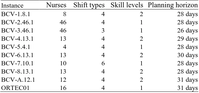
[image:5.595.134.461.573.726.2]The algorithms presented in this paper are tested on ten instances which vary in the number of nurses, cover requirements, shift types, constraint types and priorities, personal requests and planning horizon. Table 1 provides some more information on the instances.
Table 1 Problem Instances
Instance Nurses Shift types Skill levels Planning horizon
BCV-1.8.1 8 4 2 28 days
BCV-2.46.1 46 4 1 28 days
BCV-3.46.1 46 3 1 26 days
BCV-4.13.1 13 4 2 29 days
BCV-5.4.1 4 4 1 28 days
BCV-6.13.1 13 4 2 30 days
BCV-7.10.1 10 6 1 28 days
BCV-8.13.1 13 4 2 28 days
BCV-A.12.1 12 4 2 31 days
ORTEC01 16 4 1 31 days
many conflicting requests. ORTEC01 was originally presented in (Burke et al. 2008a) (an IP formulation of this instance can also be found in (Burke et al. 2008 (accepted for publication))). All these instances and the best known solutions are available at
http://www.cs.nott.ac.uk/~tec/NRP/.
3
The Variable Depth Search
Before discussing the variable depth search we will first introduce the basic neighbourhood swaps which the variable depth search uses to the form compound moves.
3.1 The Basic Search Neighbourhood
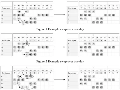
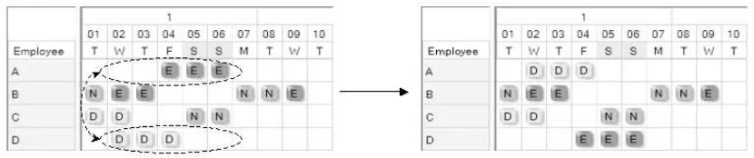
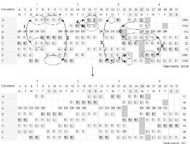
[image:6.595.91.503.415.725.2]This neighbourhood operator can de defined as swapping all the assignments between two nurses over one or more consecutive days. Examples of these swaps are given in Figures 1 to 4. The figures show a ten day section of a roster with the schedules of employees A, B, C and D visible. The labels D, E and N represent day, evening and night shifts respectively. For example, on the first day of the planning period, nurse A has a day off, nurse B has a night shift, nurse C a day shift etc. Figures 1 and 2 illustrate swaps over a period of one day. Figure 3 shows a swap over a period of three consecutive days and Figure 4 illustrates a swap over a period of five consecutive days. The number of consecutive days to try can be regarded as a parameter which can range from one up to the length of the planning period. We refer to this parameter as block length due to the block-like appearance of consecutive days in a roster.
Figure 1 Example swap over one day
Figure 2 Example swap over one day
Figure 4 Example swap over five consecutive days
3.2 The Variable Depth Search
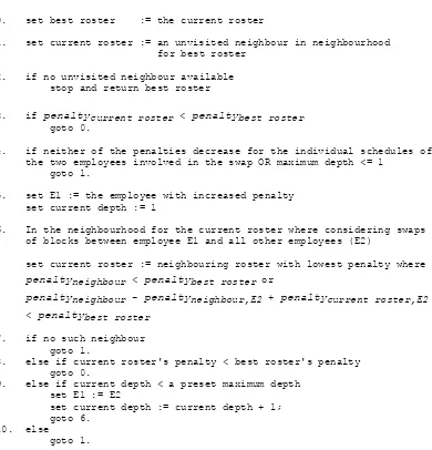
The first step of the algorithm is to create an initial roster. This is done using a randomised greedy assignment method. It operates as follows: for each shift which needs to be covered, assign it to the nurse who incurs the least gain in penalty for their schedule (or who receives the greatest decrease in penalty) on receiving this shift. In order to provide different starting solutions and allow the search to also be used with random restarts, the set of shifts to be assigned is shuffled. Once the initial roster is created, it is possible to proceed with the variable depth search. Figure 5 provides an outline of the algorithm.
Let:
penaltyr = the penalty for roster r.
penaltyr,n = the penalty for the schedule of nurse n in roster r.
0. set best roster := the current roster
1. set current roster := an unvisited neighbour in neighbourhood for best roster
2. if no unvisited neighbour available stop and return best roster
3. if penaltycurrent roster < penaltybest roster
goto 0.
4. if neither of the penalties decrease for the individual schedules of the two employees involved in the swap OR maximum depth <= 1
goto 1.
5. set E1 := the employee with increased penalty set current depth := 1
6. In the neighbourhood for the current roster where considering swaps of blocks between employee E1 and all other employees (E2)
set current roster := neighbouring roster with lowest penalty where penaltyneighbour < penaltybest roster or
penaltyneighbour - penaltyneighbour,E2 + penaltycurrent roster,E2 < penaltybest roster
7. if no such neighbour goto 1.
8. else if current roster's penalty < best roster's penalty goto 0.
9. else if current depth < a preset maximum depth set E1 := E2
set current depth := current depth + 1; goto 6.
[image:8.595.94.484.118.524.2]10. else goto 1.
Figure 5 Variable depth search outline
The neighbourhoods referred to in Figure 5 are identified by swaps of blocks up to a maximum block length (MBL). The neighbourhood at step 1 is defined by all possible swaps of blocks, on all days of the planning period, between all nurses. At step 6, the swaps are just between two nurses on all days of the planning period. It was found to be generally more efficient to set MBL at step 1 lower than at step 6 (e.g. at step 1, use two or three and at step 6, use five or six).
To further improve the performance of the algorithm another heuristic was developed to restrict the set of candidate swaps to add to the current chain. It works as follows: during penalty recalculations for a nurse’s schedule (e.g. after a swap), all days which need changing either through the removal, addition or changing of shift assignments, in order to remove a soft constraint violation are flagged. Only the swaps which involve at least one of these days are then tested. This heuristic is also applied at step 1.
3.3 Predefined Run Time
The running time for the algorithm depends on the size of the neighbourhoods at steps 1 and 6, the maximum depth used at step 9 and the structure of the instance being addressed. The size of the neighbourhoods at steps 1 and 6 depends upon the number of nurses, the number of days in the planning period and the maximum block length. The effects of the third factor (the instance structure) on the running time cannot be as easily predicted as factors such as the number of nurses and days. For some instances, it is possible that the structure (determined more by the soft constraints and their weights) is such that there is very often a valid neighbour found at step 6 with which to replace the current roster but which is not better than the best roster. This can mean that the chains examined reach great lengths which obviously affects the running time.
To reduce this effect, a maximum depth which is set beforehand is used at step 9. Initially the depth was set using a trial and error method of running the algorithm for a short time and observing its progress on the particular instance. Then altering the maximum depth value until a suitable setting is found (that is estimated) will restrict the algorithm to a satisfactory running time. This is clearly not a suitable approach for practical use. Therefore, an additional mechanism was added which takes the preferred running time as a parameter and attempts to use that time efficiently.
This mechanism works as follows: for the algorithm to finish, every neighbour in the neighbourhood at step 1 needs to be examined and potentially used as the first solution in a chain of moves. It is possible to calculate the size of the neighbourhood at step 1 using the number of nurses, the maximum block length and the number of days in the planning horizon. Given a preferred running time and the number of solutions to evaluate at step 1 (updated each time a new best solution is found), it is possible to calculate an average time to spend using each neighbour at step 1 as the first solution in a chain. Then at step 9, instead of testing whether a maximum depth will be exceeded in continuing the chain, we test whether the average time per chain will be exceeded if it continues.
Figure 6 Example chain of swaps
3.4 Hashing and Caching
Increases in performance can be achieved as effectively through making the algorithm faster and more efficient as by using better heuristics. Therefore, we will briefly discuss some implementation issues which we found significantly improved performance. At step 6, there is a possibility that a neighbouring solution will be selected that has been visited previously and cycling could occur. To prevent this we use a Zobrist (Zobrist 1970) hashing method and maintain a hash table of all previously visited solutions. A Zobrist method is particularly suited to an algorithm which makes small incremental changes to a solution. As well as avoiding cycling by using a hash table of solutions examined there are also some other efficiency measures which are worth highlighting. Firstly, when a nurse’s schedule has been altered it is only necessary to re-evaluate their schedule. Secondly, by far the most time consuming operation is calculating penalties (i.e. soft constraint evaluations). If there is a likelihood that a solution will be returned to (e.g. when reversing a chain of swaps), then the algorithm caches penalties (and violation flags) to avoid having to recalculate them. Finally, some soft constraint calculations can be speeded up by using data structures that are modified as assignments are made. A simple example is to update the total number of hours worked when a shift is (un)assigned rather than to add all the hours up when calculating the penalty. Some of the more complicated constraints benefit from a similar approach.
4
Results
previously published approaches. The experiments were performed using a desktop PC with an Intel P4 2.4GHz processor.
Brucker et al. (Brucker et al. 2009) developed a heuristic constructive approach and tested it on the benchmark instances. As it is a constructive method it is not possible to provide a comparison to the variable depth search by using the number of solutions examined metric. However, their experiments were performed on the same machine and a comparison can be provided by using computation times. The results in Table 2 are Brucker et al’s best results from all experiments. The total computation time in obtaining these solutions for each instance was then set as the maximum run time for the variable depth search.
[image:11.595.121.478.289.452.2]Burke et al’s (Burke et al. 2008a) result for ORTEC01 using the hybrid variable neighbourhood search had a computation time of twelve hours. The result for the variable depth search on this instance is the best of five, five minute tests.
Table 2 Comparison of VDS with two other algorithms
Time
(Brucker et al. 2009)
(Burke et al.
2008a) Variable depth search
ORTEC01 12 hrs - 541 360
BCV-1.8.1 136 sec 323 - 253
BCV-2.46.1 3424 sec 1594 - 1572
BCV-3.46.1 2888 sec 3601 - 3324
BCV-4.13.1 208 sec 18 - 10
BCV-5.4.1 16 sec 200 - 48
BCV-6.13.1 304 sec 890 - 768
BCV-7.10.1 216 sec 396 - 381
BCV-8.13.1 224 sec 148 - 148
BCV-A.12.1 944 sec 3335 - 1843
As can be seen, the variable depth search outperforms the constructive method, over the same computation times, on all instances except one, on which they are equal. It also beats the hybrid method of Burke et al. on instance ORTEC01.
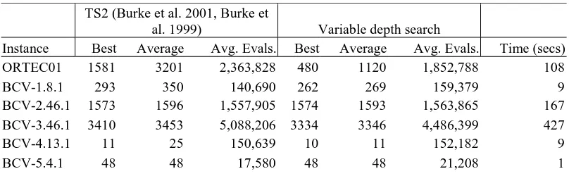
To provide further comparisons, the hybrid tabu search of Burke et al. (Burke et al. 2001, Burke et al. 1999) was implemented and tested on the benchmark data sets. The best version of their tabu search (TS2) was applied five times to each instance. Table 3 contains the best and average results. The average execution time on each instance was also recorded. The variable depth search was then set a maximum run time identical to that used by the tabu search for each instance. Five repeats of the variable depth search were then performed to obtain average and best results.
Table 3 Comparison of the variable depth search with a hybrid tabu search
TS2 (Burke et al. 2001, Burke et
al. 1999) Variable depth search
Instance Best Average Avg. Evals. Best Average Avg. Evals. Time (secs)
ORTEC01 1581 3201 2,363,828 480 1120 1,852,788 108
BCV-1.8.1 293 350 140,690 262 269 159,379 9
BCV-2.46.1 1573 1596 1,557,905 1574 1593 1,563,865 167 BCV-3.46.1 3410 3453 5,088,206 3334 3346 4,486,399 427
BCV-4.13.1 11 25 150,639 10 11 152,182 9
[image:11.595.96.500.638.763.2]BCV-6.13.1 1010 1154 345,595 769 817 356,891 24
BCV-7.10.1 391 458 93,817 381 427 117,224 7
BCV-8.13.1 148 165 215,524 148 148 248,927 15
BCV-A.12.1 2065 2831 718,354 1835 1942 649,926 108
As shown in Table 2 and Table 3 the variable depth search nearly always outperforms or equals the other methods in comparable tests over all instances. The only time it was beaten was when TS2 found a best solution for BCV-2.46.1 with penalty 1573. The variable depth search could still manage a best with penalty 1574 though. Note also that the variable depth search is actually dynamically adjusting to the run time of the other approaches.
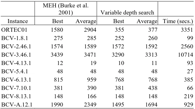
[image:12.595.140.456.425.602.2]For a final comparison, the variable depth search was compared against the memetic algorithm, MEH, of Burke et al (Burke et al. 2001). MEH is a hybrid approach which performs a tabu search on individuals in the population between generations and a greedy shuffling step on the best solution at the end. It was shown to be a robust approach and the best method on more difficult instances. The same settings as described in the original paper were used (underlying memetic algorithm ME4, population size of twelve and stop criterion of no improvement during two generations). Five repeats of the algorithm were executed and the best and average solutions and average computation times were recorded. The variable depth search was then assigned a pre-defined maximum run time equal to the average time used by MEH for each instance and five runs also performed. The best and average results for both algorithms are shown in Table 4.
Table 4 Comparison of the variable depth search with a memetic algorithm
MEH (Burke et al.
2001) Variable depth search
Instance Best Average Best Average Time (secs.)
ORTEC01 1580 2904 355 377 3351
BCV-1.8.1 275 285 252 260 99
BCV-2.46.1 1574 1589 1572 1592 2560
BCV-3.46.1 3439 3471 3290 3313 10714
BCV-4.13.1 12 19 10 11 93
BCV-5.4.1 48 48 48 48 27
BCV-6.13.1 815 959 768 768 385
BCV-7.10.1 381 390 381 438 66
BCV-8.13.1 148 166 148 148 219
BCV-A.12.1 1990 2349 1495 1694 929
Comparing against MEH using average results, the variable depth search outperforms on seven of the ten instances, is equal on one and worse on the other two. Using best results, VDS is better on seven out of ten instances and equal on three. Again, the variable depth search is very competitive even when adjusting to the run times of the other algorithm.
5
Conclusions
order to escape the local optima they would otherwise be limited to. The key to its success are the rules and heuristics for deciding whether to continue a chain and which candidate swaps to examine as the next link in the chain. When compared against previously published algorithms using real world benchmark data sets it has been shown to be a very effective approach. To make the algorithm even more applicable to practice, we have suggested a simple but effective mechanism that dynamically adjusts the algorithm to a pre-defined maximum run time.
Although we believe the algorithm is relatively straightforward to understand it should also be noted it is not trivial to implement and has a significant potential for bugs. However, we have highlighted some ideas which we used to achieve a fast and efficient implementation.
There also a few possibilities for future work. It may be possible to develop a more powerful algorithm by using the variable depth search as the improvement method in a population based approach such as a memetic algorithm (Krasnogor and Smith 2005) or a scatter search (Glover et al. 2000). Additionally, we observed specific swap block lengths are particularly effective on certain instances. A method which can exploit this by, for example, intelligently selecting this parameter, may be able to contribute gains in performance. One possibility may be an algorithm which runs some short preliminary tests on the instance, testing different values in order to estimate the best parameter. An alternative approach may be to dynamically adjust the algorithm’s parameters as the search progresses. This is somewhat akin to hyperheuristics (Burke et al. 2003, Ross 2005).
All the test instances and best solutions are publicly available at the research website:
http://www.cs.nott.ac.uk/~tec/NRP/. We also plan to create more data sets taken from real world rostering scenarios which along with any new best known solutions will be published at the same location.
Acknowledgements
This work was supported by EPSRC grant GR/S31150/01.
References
Abdullah S, Ahmadi S, Burke E K and Dror M. 2007a. Investigating Ahuja-Orlin's Large Neighbourhood Search Approach for Examination Timetabling. OR Spectrum29(2) 351-372.
Abdullah S, Ahmadi S, Burke E K, Dror M and McCollum B. 2007b. A tabu-based large neighbourhood search methodology for the capacitated examination timetabling problem. Journal of the Operational Research Society 58 1494– 1502.
Ahuja R K, Ergun Ö, Orlin J B and Punnen A P. 2002. A survey of very large-scale neighborhood search techniques. Discrete Applied Mathematics 123(1-3) 75-102.
Aickelin U, Burke E K and Li J. 2007. An Estimation of Distribution Algorithm with Intelligent Local Search for Rule-based Nurse Rostering. Journal of the Operational Research Society58(12) 1574-1585.
Aickelin U and Li J. 2007. An Estimation of Distribution Algorithm for Nurse Scheduling. Annals of Operations Research155(1) 289-309.
Azaiez M N and Al Sharif S S. 2005. A 0-1 goal programming model for nurse scheduling. Computers and Operations Research32(3) 491 - 507.
Bard J F and Purnomo H W. 2007. Cyclic Preference Scheduling of Nurses Using A Lagrangian-Based Heuristic. Journal of Scheduling10(1) 5-23.
Beddoe G R and Petrovic S. 2006. Selecting and Weighting Features Using a Genetic Algorithm in a Case-Based Reasoning Approach to Personnel Rostering.
European Journal of Operational Research175(2) 649-671.
Beddoe G R and Petrovic S. 2007. Enhancing case-based reasoning for personnel rostering with selected tabu search concepts. Journal of the Operational Research Society58 1586–1598.
Bellanti F, Carello G, Croce F D and Tadei R. 2004. A greedy-based neighborhood search approach to a nurse rostering problem. European Journal of Operational Research153 28–40.
Berrada I, Ferland J A and Michelon P. 1996. A multi-objective approach to nurse scheduling with both hard and soft constraints. Socio-Economic Planning Sciences30(3) 183-193.
Bourdais S, Galinier P and Pesant G. 2003. HIBISCUS: A Constraint Programming Application to Staff Scheduling in Health Care. In: CP 2003, Lecture Notes in Computer Science 2833, 153-167.
Brucker P, Burke E K, Curtois T, Qu R and Vanden Berghe G. 2009. A Shift Sequence Based Approach for Nurse Scheduling and a New Benchmark Dataset. Journal of Heuristics16(4) 559-573.
Burke E K, Cowling P, De Causmaecker P and Vanden Berghe G. 2001. A Memetic Approach to the Nurse Rostering Problem. Applied Intelligence 15(3) 199-214.
Burke E K, Curtois T, Post G, Qu R and Veltman B. 2008a. A Hybrid Heuristic Ordering and Variable Neighbourhood Search for the Nurse Rostering Problem. European Journal of Operational Research188(2) 330-341.
Burke E K, Curtois T, Qu R and Vanden Berghe G. 2008b. Problem Model for Nurse
Rostering Benchmark Instances. from
http://www.cs.nott.ac.uk/~tec/NRP/papers/ANROM.pdf.
Burke E K, De Causmaecker P, Petrovic S and Vanden Berghe G. 2004a. Variable Neighborhood Search for Nurse Rostering Problems. In: Resende M G C and de Sousa J P (eds). Metaheuristics: Computer Decision-Making. Kluwer Norwell, MA, USA, 153-172.
Burke E K, De Causmaecker P and Vanden Berghe G. 1999. A Hybrid Tabu Search Algorithm for the Nurse Rostering Problem. In: McKay B, X. Yao, Newton C S, Kim J and Furuhashi T (eds). Simulated Evolution and Learning, Selected Papers from the 2nd Asia-Pacific Conference on Simulated Evolution and Learning, SEAL 98, Springer Lecture Notes in Artificial Intelligence Volume 1585. Springer-Verlag London UK, 187-194.
Burke E K, De Causmaecker P, Vanden Berghe G and Van Landeghem H. 2004b. The State of the Art of Nurse Rostering. Journal of Scheduling7(6) 441 - 499. Burke E K, Kendall G and Soubeiga E. 2003. A Tabu-Search Hyperheuristic for
Timetabling and Rostering. Journal of Heuristics9(6) 451 - 470.
Darmoni S J, Fajner A, Mahé N, Leforestier A, Vondracek M, Stelian O and Baldenweck M. 1995. Horoplan: computer-assisted nurse scheduling using constraint-based programming Journal of the Society for Health Systems5 41-54.
Dias T M, Ferber D F, de Souza C C and Moura A V. 2003. Constructing nurse schedules at large hospitals. International Transactions in Operational Research10(3) 245-265.
Dowsland K A. 1998. Nurse scheduling with tabu search and strategic oscillation.
European Journal of Operational Research106(2) 393-407.
Ernst A T, Jiang H, Krishnamoorthy M, Owens B and Sier D. 2004. An Annotated Bibliography of Personnel Scheduling and Rostering. Annals of Operations Research127 21–144.
Glover F. 1996. Ejection Chains, Reference Structures and Alternating Path Methods for Traveling Salesman Problems. Discrete Applied Mathematics65(1-3) 223-253.
Glover F, Laguna M and Martí R. 2000. Fundamentals of scatter search and path relinking. Control and Cybernetics29(3) 653-684.
Jaszkiewicz A. 1997. A metaheuristic approach to multiple objective nurse scheduling. Foundations of Computing and Decision Sciences22(3) 169-183. Jaumard B, Semet F and Vovor T. 1998. A Generalized Linear Programming Model
for Nurse Scheduling. European Journal of Operational Research 107(1) 1-18.
Krasnogor N and Smith J. 2005. A Tutorial for Competent Memetic Algorithms: Model, Taxonomy and Design Issues. IEEE Transactions on Evolutionary Computation9(5) 474-488.
Lin S and Kernighan B W. 1973. An Effective Heuristic Algorithm for the Traveling-Salesman Problem. Operations Research21(2) 498-516.
Louw M J, Nieuwoudt I and Van Vuuren J H. 2005. Finding Good Nursing Duty Schedules: A Case Study. Technical Report, Department of Applied Mathematics, Stellenbosch University, South Africa.
Mason A J and Smith M C. 1998. A Nested Column Generator for solving Rostering Problems with Integer Programming. In: Caccetta L, Teo K L, Siew P F, Leung Y H, Jennings L S and Rehbock V (eds). International Conference on Optimisation: Techniques and Applications, Perth, Australia, 827-834.
Meisels A, Gudes E and Solotorevsky G. 1995. Employee Timetabling, Constraint Networks and Knowledge-Based Rules: A Mixed Approach. In: Burke E and Ross P (eds). Selected papers from the First International Conference on Practice and Theory of Automated Timetabling, Springer Lecture Notes in Computer Science Volume 1154, 93-105.
Meisels A and Schaerf A. 2003. Modelling and solving employee timetabling problems. Annals of Mathematics and Artificial Intelligence39 41-59.
Meyer auf'm Hofe H. 2000. Solving Rostering Tasks as Constraint Optimization. In: Burke E K and Erben W (eds). Selected papers from the Third International Conference on Practice and Theory of Automated Timetabling, Springer Lecture Notes in Computer Science Volume 2079 Springer-Verlag Berlin Heidelberg, 191-212.
Miller H E, Pierskalla W P and Rath G I. 1976. Nurse Scheduling Using Mathematical Programming. Operations Research24(5) 857-870.
Pesch E and Glover F. 1997. TSP ejection chains Discrete Applied Mathematics 76
165-181.
Rego C. 1998. A Subpath Ejection Method for the Vehicle Routing Problem.
Management Science44(10) 1447-1459.
Ross P. 2005. Hyper-heuristics. In: Burke E K and Kendall G (eds). Search Methodologies: Introductory Tutorials in Optimization and Decision Support Techniques. Springer, 529-556.
Thornton J and Sattar A. 1997. Nurse Rostering and Integer Programming Revisited. In: Verma B and Yao X (eds). International Conference on Computational Intelligence and Multimedia Applications. Griffith University Gold Coast, Australia, 49-58.
Valouxis C and Housos E. 2000. Hybrid optimization techniques for the workshift and rest assignment of nursing personnel. Artificial Intelligence in Medicine
20 155-175.
Vanden Berghe G. 2002. An Advanced Model and Novel Meta-Heuristic Solution Methods to Personnel Scheduling in Healthcare, University of Gent, Belgium. Ph.D. Thesis.
Warner D M. 1976. Scheduling Nursing Personnel according to Nursing Preference: A Mathematical Programming Approach Operations Research24 842-856. Yagiura M, Yamaguchi T and Ibaraki T. 1999. A Variable Depth Search Algorithm
for the Generalized Assignment Problem. In: Voss S, Martello S, Osman I H and Roucairol C (eds). Meta-Heuristics: Advances and Trends in Local Search Paradigms for Optimization. Kluwer Academic Publishers Boston, MA, 459-471.