SWIFF : space weather integrated forecasting framework

SWIFF: Space weather integrated forecasting framework

Giovanni Lapenta

, Viviane Pierrard

, Rony Keppens

, Stefano Markidis

, Stefaan Poedts

, Ondrˇej Sˇebek

,

Pavel M. Tra´vnı´cˇek

, Pierre Henri

, Francesco Califano

, Francesco Pegoraro

, Matteo Faganello

Vyacheslav Olshevsky

, Anna Lisa Restante

, A

˚ ke Nordlund

_{, Jacob Trier Frederiksen}

_{, Duncan H. Mackay}

_,

Clare E. Parnell

, Alessandro Bemporad

, Roberto Susino

, and Kris Borremans

1 _{Centre for mathematical Plasma Astrophysics, Department of Mathematics, KU Leuven, Celestijnenlaan 200B,}

3001 Leuven, Belgium

*_{corresponding author: e-mail:[email protected]} 2

Belgian Institute for Space Aeronomy, Space Physics, 3 ringlaan, B-1180 Brussels, Belgium 3

Astronomical Institute, Institute of Atmospheric Physics, AS CR, Bocˇnı´ II 1401, 14131 Prague, Czech Republic 4

Space Sciences Laboratory, University of California Berkeley, 7 Gauss Way, Berkeley, CA 94720, USA 5

Dipartimento di Fisica, Universita di Pisa, Largo Pontecorvo 3, 56127 Pisa, Italy 6

Laboratoire de PIIM, UMR 6633, CNRS, Aix-Marseille Universite, Marseille, France 7

Niels Bohr Institute, University of Copenhagen, Juliane Maries Vej 3, DK-2100 Copenhagen, Denmark 8

School of Mathematics & Statistics, University of St Andrews, North haugh, St Andrews, Fife KY16 9SS, Scotland 9

INAF – Turin Astronomical Observatory, via Osservatorio 20, 10025 Pino Torinese (TO), Italy 10

INAF – Catania Astrophysical Observatory, via S. Sofia 78, 95123 Catania, Italy 11

Main Astronomical Observatory, NAS of Ukraine, Zabolotnoho 27, 03680 Kyiv, Ukraine 12

PDC Center for High Performance Computing, KTH Royal Institute of Technology, Stockholm, Sweden

Received 1 May 2012 / Accepted 27 January 2013

ABSTRACT

SWIFF is a project funded by the Seventh Framework Programme of the European Commission to study the mathematical-physics models that form the basis for space weather forecasting. The phenomena of space weather span a tremendous scale of densities and temperature with scales ranging 10 orders of magnitude in space and time. Additionally even in local regions there are con-current processes developing at the electron, ion and global scales strongly interacting with each other. The fundamental challenge in modelling space weather is the need to address multiple physics and multiple scales. Here we present our approach to take exist-ing expertise in fluid and kinetic models to produce an integrated mathematical approach and software infrastructure that allows fluid and kinetic processes to be modelled together. SWIFF aims also at using this new infrastructure to model specific coupled processes at the Solar Corona, in the interplanetary space and in the interaction at the Earth magnetosphere.

Key words.space weather – modelling – high performance computing

1. Introduction

Space weather refers to a complex state resulting from the Sun activity, propagating in the interplanetary space and possibly affecting the Earth space environment, which all together can influence, not only the performance and reliability of space-borne and ground-based technological systems, but more signif-icantly can endanger human life or health. Adverse conditions in the space environment can cause disruption of satellite oper-ations, communicoper-ations, navigation, and electric power distri-bution grids, leading to a variety of socioeconomic losses. In addition, the space weather influences the Earth climate. It is well known that solar activity affects the total amount of heat and light reaching the Earth and the amount of cosmic rays arriving in the atmosphere, directly contribute to a phenomenon responsible for the amount of cloud cover and precipitation. Given these crucial impacts on society, the space weather is attracting a growing worldwide attention and progressively increases presence within international research projects.

SWIFF (Space Weather Integrated Forecasting Framework) aims at creating a mathematical model and a software

infrastructure able to describe and predict the physical processes in the magnetized plasma all the way between the Sun and Earth. It aims at coupling different regions of space to produce tools that would rise space weather forecasting to qualitatively new level. The principal difference of SWIFF with respect to other similar efforts within Europe, USA and Japan, is the final goal: to create a new modelling framework based on both kinetic and fluid treatments of plasma.

We focus here on the steps necessary for achieving a true physics-based capability to predict the arrival and consequences of major space weather storms. Great disturbances in the space environment are common but their precise arrival and impact on human activities vary greatly. Simulating such a system is a grand challenge, requiring computing resources at the limit of what is possible, not only with current technology, but also with the foreseeable future generations of supercomputers.

The actors of space weather are the Sun, the Earth and the vast space in between. Like any star, the Sun is made of a highly energetic and highly conductive gas, called plasma. In plasmas, the atoms have been broken into their nuclei and their

J. Space Weather Space Clim.3 (2013) A05 DOI:10.1051/swsc/2013027

G. Lapenta et al., Published byEDP Sciences2013

O

A

R

A

electrons that become free to move. The hot plasma of the Sun is confined by gravity and moves in complex patterns that pro-duce large currents and large magnetic fields. The gravitational confinement is not perfect and a highly varying outflow of plasma, called solar wind, is emitted from the Sun to permeate the whole solar system, reaching the Earth. The Earth has itself a magnetic field. The Earth magnetic field makes compasses point towards the North Pole and allows many species of animals to find their way during migrations. This very same field protects the Earth from the incoming solar wind and its disturbances. Only a small fraction of the particles can reach the Earth surface, the so-called cosmic rays. Most of the incom-ing plasma is stopped and deflected, reachincom-ing only high strata of the atmosphere at the polar regions and causing the aurora seen by the people, normally residing at high latitudes, as either the northern or southern lights.

To describe and predict such space weather processes, both electromagnetic fields and plasma particles need to be modeled and simulated. The nuclei (mostly protons, the nuclei of hydro-gen) and the electrons of the plasma are loosely coupled, where each species has its own typical scales. The electromagnetic fields keep the species coupled forming a very nonlinear and multi-scale system. Modeling space weather is a daunting task: daunting because the system is enormous and because it includes a wide variety of physical processes and of time-and space scales. Figure 1 shows the typical physical scales observed from space exploration missions in the Earth environ-ment. The scales are presented in the form of a hourglass with the top part presenting the macroscopic scales of evolution and at the bottom the smallest microscopic scales important to be coupled together with macroscopic once.

The fundamental goal of the SWIFF project is to progress beyond the state of the art in two ways. First, in the develop-ment of mathematical models and computational methods and software especially designed to handle the multiple physics and the multiple scales characteristic of space weather phenom-ena. The project intends to produce an integrated forecasting framework able to model space weather events from their solar

origin to the impact on Earth and its space environment, focus-ing on the effect on human befocus-ings and technology in space and on the ground infrastructure. Second, we intend to demonstrate for practical space weather events and processes the validity and usefulness of the SWIFF integrated space weather forecast-ing framework. Our study will include all phases of space weather events and will push forward the state of the art in modeling specific space weather events and processes.

Fig. 1. Multi-level-Multi-physics approach.Left: domains on different levels can move and interchange information to follow the self-consistent evolution of the features they model. The different considered levels are the following. Coarsest: plasma treated as a single fluid. Intermediate levels account for multi-fluid approaches (Hall MHD, electron MHD or two fluid) or hybrid (electrons are treated as a fluid but ions are treated kinetically). Finest level: kinetic electrons and ions, both treated as particles. The multi-level approach allows to push beyond the state of the art and model all coupled scales together. The scales are indicated here for the Earth’s magnetotail, as an example.

SWIFF’s approach is different from that of other previous efforts. The goal of SWIFF is not to join existing codes to cre-ate a modeling tool that tracks space weather events from source on the Sun to the effects on the Earth. That approach has already been taken by previous successful efforts, such as Community Coordinated Modeling Center (CCMC)1 and Space Weather Modeling Framework (SWMF) (To´th et al. 2005), and it is not replicated by SWIFF. The approach of SWIFF is to recognize that to track successfully space weather processes, there are a few crucial steps where multiple scales become critically linked. These are shocks, interfaces and reconnection regions. There the electron, ion and global scales become linked. The present paper focuses on reconnection regions. There the global field topology changes via processes that happen at the local electron scales with the particles being accelerated to speeds far exceeding the Alfve´n speed. SWIFF aims at creating an integrated framework able to treat these cou-pled processes: electron, ion and magnetohydrodynamics (MHD) scales. These three scales need different physics approaches: fully kinetic at the electron scales, MHD at the glo-bal scale and hybrid or other advanced fluid methods at the ion scales. This approach is described here and it is demonstrated to the specific case of reconnection regions.

2. Integrated modeling of space weather

The study of space weather confronts researchers with the need for two types of integrations.

First, the need is present to cover a wide range of different physical and chemical processes to describe such widely differ-ent systems as the solar photosphere, the corona, the interplane-tary space, the Earth environment down to the Earth ionosphere and upper atmosphere. Future work will need also to consider the coupling with climate models of the Earth. This integration of models requires to federate existing models developed by dif-ferent teams with a background over difdif-ferent disciplines.

Second, the need is present, even within a given physical region to treat different scales with different models. Often in

space weather events, local dissipations are caused by overall macroscopic evolution and in turn enable paths and processes not possible without the microphysics. As an example, the pro-cess of magnetic reconnection bases its effectiveness on the presence of microscopic processes that dissipate energy and enable macroscopic changes of the magnetic field configura-tion. This micro-macro coupling requires to couple fluid models valid for macroscopic processes with kinetic models required for the proper treatment of the microphysics.

The approach of SWIFF is different from other previous similar enterprises. SWIFF does not focus on linking existing tools and codes. Rather SWIFF explores integrated mathemat-ical models where different physmathemat-ical processes and different scales are treated within the same approach. SWIFF federates different areas of expertise, bringing in experts and models from all aforementioned areas of research following the evolution of space weather events from the Sun to the Earth. But the main peculiarity of SWIFF, one that sets it apart from other previous space weather modelling effort, is to make its primary aim that of finding an effective way to couple fluid and kinetic models for micro-macro simulation.

The kinetic approach is more computationally expensive, as it concentrates on microscopic scales, and its use is limited to small regions of space. Conversely, the fluid model (called magnetohydrodynamics, MHD) is valid throughout most of the system of interest but fails in small regions where extreme conditions are found and strong processes of energy conversion and plasma instabilities are present. Only coupling the two approaches as SWIFF is doing can allow a feasible physics-based description of space weather.

The SWIFF approach to reach this goal is the use of adap-tive grid methods to address the multi-scale challenge in the spatial domain, the use of implicit time differencing to address the multi-scale challenge in the time domain and to use moment methods and coupled multi-layer simulations to interface domain characterized by different physical description (fund or kinetic). Below the research in these three areas is reviewed, giving a brief introduction to the existing literature but focusing on the methods used within SWIFF.

2.1. Adaptive spatial resolution

Modern fluid-based space weather simulations routinely exploit Adaptive Mesh Refinement (AMR), where hierarchically nested grids of increasing spatial resolution trace distinct flow features. The adaptivity can dynamically improve or sacrifice local grid resolution using a mixture of physics- and accu-racy-based criteria. While AMR exists in many varieties, going from cell-based, over patch-based to block-based refinement strategies, especially the block-based octree variant is very well suited for massive parallel computations, where each time step, the parallelism over the many blocks to be advanced can effi-ciently be exploited. This strategy is used in a fair variety of open source astrophysically oriented software packages, such as FLASH Calder et al. (2002), NIRVANA Ziegler (2005), RAMSESFromang et al. (2006). For space weather oriented applications, AMR features as a crucial ingredient within codes employed in current modelling frameworks, such as the Space Weather Modeling Framework To´th et al. (2005). A recent review of the means to handle different physics, multi-scale problems with this framework, as well as an overview of the AMR kernel employed in their main BATS-R-USPowell et al. (1999)code, is found inTo´th et al. (2012).

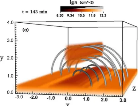
Fig. 3. A 3D view on the prominence formed due to the thermal instability on top of a sheared magnetic arcade (as shown in field lines). A volume rendering of the density shows the low-lying denser chromospheric regions, as well as the prominence matter. The simulation was performed with MPI-AMRVAC code.

1

Within the SWIFF project, we continuously develop and exploit the MPI-AMRVAC codeKeppens et al. (2003,2012), where a dimension-independent block-based AMR is imple-mented using the LASY syntaxTo´th (1997), and the distribu-tion of the blocks over the CPUs is handled through a Morton-ordered space filling curve through the dynamically changing grid hierarchy. MPI-AMRVAC offers flexibility in selecting/augmenting the refinement (unrefinement) criteria, can handle Cartesian, cylindrical and spherical geometries, and can readily simulate systems of (hyperbolic) partial differ-ential equations (PDEs), as e.g., encountered in multi-dimen-sional magnetohydrodynamics. The code has played a role within the SWIFF collaboration to benchmark simulation chal-lenges used to intercompare the network toolpark. As an illus-trative example which is discussed further on in this paper,

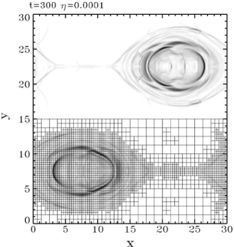
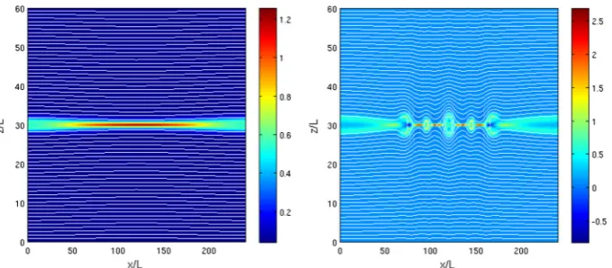
Figure 2shows the instantaneous density variation in a resistive evolution of a reconnecting current sheet. The figure uses a schlieren representation (i.e., an exponentially stretched quanti-fication of the local density gradient) for a 2D fully periodic test case of a double Harris current sheet setup. A resistive MHD simulation with resistivity parameter g = 0.0001 follows the evolution of these current sheets when subjected to initial per-turbations. At sufficient resolution, one witnesses how they transit to fast reconnection regimes where repeated islands form along the thinning central current sheets. These islands merge chaotically with the main island structures connecting to these sheets. This simulation has exploited only five AMR grid levels with a base resolution of 60·60 realizing a 960·960 effec-tive resolution. The adaptivity uses an instantaneous estimate of the second derivatives, weighing in density and magnetic field components, and it is important to note that this long-term sim-ulation can be done on a local four CPU desktop in a matter of hours. The grid structure evolves from about 600 grid blocks (of size 10·10) initially, when only exploiting four out of five grid levels, to about 5300 grid blocks at the time depicted. The grid structure is shown in the bottom half of the graph and dem-onstrates how the grid traces the evolving dynamics accurately. At this time (timet= 300 in code units), only the three highest grid levels are actually present, and the evolution maintains a high level of symmetry throughout.

An example application using the automated AMR approach is shown inFigure 3. This shows a snapshot of a pio-neering simulation of prominence formation in the solar corona

Xia et al. (2012), where the prominence can be seen as a density enhancement forming an elongated sheet of cold, dense matter residing on top of a magnetic arcade (for which selected field lines are shown). This magnetohydrodynamic simulation encounters a multi-scale challenge due to the need to resolve the dramatic thermodynamic changeover from low chromo-spheric to high coronal regions (seen in density at the bottom of the figure), as well as to temporally follow the localized instability development due to optically thin radiative losses. Prior investigations restricted to one space dimension (along rigid field lines) already demonstrated the need for AMRXia et al. (2011),Antiochos et al. (1999), but only by tackling the multi-dimensional problem can the backreaction on the mag-netic field, seen in the figure to induce a dipped concave upward configuration, be captured. It was further shown that while the prominence grows to macroscopic dimensions, force balance is achieved throughout. This paves the way for future investigations where solar coronal mass ejection simulations can be initiated with more realistic, prominence carrying mag-netic configurations. While the configuration shown inFigure 3

does not involve reconnecting field lines, scenarios for forming

flux-rope embedded filaments can be envisaged where also magnetic reconnection plays an essential role. In that sense, the possibility to handle the evolution of multiple physical mechanisms on a multi-scale with AMR capabilities will prove crucial.

Both examples given thus far still adopt a single fluid MHD description, while incorporating deviations from ideal MHD through locally important resistive and/or thermodynamic pro-cesses (heat gain/loss and anisotropic thermal conduction). At a next level of sophistication, we explored coupling strategies for different hyperbolic PDEs on hierarchically nested configu-rations (Keppens & Porth 2012, submitted). This would be needed when coupling single fluid MHD evolutions to a sequence of Hall-MHD and increasingly elaborate two-fluid formulations. Using a model scalar nonlinear PDE, this kind of coupling was found to be liable to the creation of local dis-continuities at the fixed model transition boundaries when insisting on perfect conservation, or lead to non-conservative, but intuitively consistent evolutions without such artefacts. On the basis of these experiments, a Hall-MHD module has been incorporated in MPI-AMRVAC, with the aim to revisit several of the reconnection challenges described further on, where both ideal, resistive, to Hall- MHD regions appear concurrently.

2.2. Implicit temporal discretization and the moment method

When the governing equations of fluid and kinetic approaches are discretized in time, the explicit and implicit methods can be used. The explicit temporal discretization leads to fairly simple numerical schemes that require a reduced number of computa-tions. Because explicit techniques are conceptually simple and

have straightforward implementation, many fluid and kinetic codes use explicit discretization of the governing equations. However, explicit methods are numerically unstable when the simulation time step and grid spacing exceed certain values. These values are so small that explicit fluid simulations require a huge number of computational cycles with small time step and grid spacing and explicit kinetic simulations for space weather are not feasible (not even on the current fastest super-computers). The implicit method solves the problem of the small time steps and grid spacings: it completely removes the stability constraints of the explicit methods, allowing the user to choose the most convenient time step and grid spacing for studying a given space weather phenomenon.

Fluid simulations benefit from fully implicit approaches. Pioneering work in implicit MHD treatments shows that it is possible to step over fast time scales without compromising accuracy or efficiency, reporting CPU speed-ups of implicit ver-sus explicit methods of an order of magnitude. In the context of multiple scale modeling where the kinetic scale has to be con-sidered, the limitations arising with the use of explicit methods in the treatment of fluid models become a minor consideration when compared with the limits imposed by the explicit differ-entiation of the kinetic equations. In fact, two constraints need to be satisfied in kinetic explicit modeling. First, the time step needs to be smaller than the fastest time scale (typically the plasma frequency), which may be orders of magnitude faster than the dynamical time scale of interest. Second, the simula-tion grid spacing needs to resolve the smallest spatial scale, the Debye length, that is typically several orders of magnitude

smaller than the other scales of interest. Given these limitations, 3D explicit fully kinetic simulations for realistic choice of parameters will remain out of reach in the foreseeable future. Therefore, we have taken a different approach in SWIFF: we use implicit time differencing for kinetic simulation. Implicit kinetic methods have been shown to be free from both spatial and temporal limitations, and as a consequence have been able to push the limits of plasma physics simulation to regimes where explicit methods have not been able to reach, even with the use of powerful supercomputers.

Implicit kinetic plasma simulation has taken essentially two lines of investigation that over the years have converged to a similar framework and the distinction has become largely of historical interest. The two approaches are: the direct implicit method Hewett & Langdon (1987) and the implicit moment methodBrackbill & Cohen (1985),Ricci et al. (2002),Lapenta et al. (2006),Lapenta (2012). Both techniques led to well-estab-lished codes with a wealth of applications. The first method has been developed primarily at Lawrence Livermore National Lab-oratory (LLNL) and the second has been developed primarily at the Los Alamos National Laboratory (LANL). The SWIFF effort takes full advantage of all the progress made to date on each of the methods, but will rely primarily on the implicit moment method for two reasons. The first is practical, some SWIFF proponents have been long involved in the develop-ment of the method and of the modern codes based on them. The second is theoretical: the computational engine of the implicit moment method already includes the solution of the kinetic and fluid equations. In fact, the implicit moment method

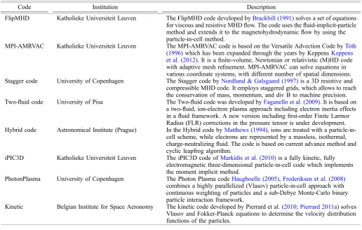
Table 1.Numerical codes available to the member institutions of SWIFF consortium.

Code Institution Description

FlipMHD Katholieke Universiteit Leuven The FlipMHD code developed byBrackbill (1991)solves a set of equations for viscous and resistive MHD flow. The code uses the fluid-implicit-particle method and extends it to the magnetohydrodynamic flow by using the particle-in-cell method.

MPI-AMRVAC Katholieke Universiteit Leuven The MPI-AMRVAC code is based on the Versatile Advection Code byTo´th (1996)which has been expanded through the years by KeppensKeppens et al. (2012). It is a finite-volume, Newtonian or relativistic (M)HD code with adaptive mesh refinement. MPI-AMRVAC can solve equations in various coordinate systems, with different number of spatial dimensions. Stagger code University of Copenhagen The Stagger code byNordlund & Galsgaard (1997)is a 3D resistive and

compressible MHD code. It employs staggered grids, which allows to reach the conservation of mass, momentum, and div B to machine precision. Two-fluid code University of Pisa The Two-fluid code was developed byFaganello et al. (2009). It is based on

a two-fluid, ion-electron plasma approach including electron inertia effects in a fluid framework. A new version including first-order Finite Larmor Radius (FLR) corrections in the pressure tensor is under development. Hybrid code Astronomical Institute (Prague) In the Hybrid code byMatthews (1994), ions are treated with a

particle-in-cell scheme, while electrons are represented by a massless, isothermal, charge-neutralizing fluid. The code is based on current advance method and cyclic leapfrog algorithm.

iPIC3D Katholieke Universiteit Leuven The iPIC3D code ofMarkidis et al. (2010)is a fully kinetic, fully electromagnetic three-dimensional particle-in-cell code which implements the moment implicit method.

PhotonPlasma University of Copenhagen The Photon Plasma codeHaugboelle (2005),Frederiksen et al. (2008)

combines a highly parallelized (Vlasov) particle-in-cell approach with continuous weighting of particles and a sub-Debye Monte-Carlo binary particle interaction framework.

is based on solving the kinetic equations by coupling them with the moment equations (i.e., with fluid equations): since the method is based both on the kinetic and the fluid approaches, it is naturally suited to handle the task of using fluid equations in some regions and kinetic equations in other. The implicit moment PIC method has already provided a unified modelling framework for the concurrent solution of kinetic and fluid equations.

2.3. Multi-physics-multi-level description

In typical space conditions, the nonlinear dynamics of magne-tized plasmas is driven by the energy injected at the large, fluid scales. This energy is then transferred self-consistently towards smaller and smaller scales, until kinetic effects come into play. The plasma turbulent cascade routinely observed by satellites in the solar wind is an archetype of such multi-scale behaviour

Bruno & Carbone (2005), Valentini et al. (2010), but many other space plasma processes exhibit a similar behaviour. At the interface between two different plasma regions, e.g. between the magnetosphere and the solar wind, large-scale, fluid instabilities self-consistently build up complex dynamics where kinetic processes play a key role. This is the case for instance at the transition region between the solar wind flowing plasma and the magnetosphere plasma at rest at low latitude nearby the equatorial plane (more precisely the magneto-sphere-magnetosheath interface), where the velocity shear between these plasmas is an efficient source for the develop-ment of the Kelvin-Helmholtz instability. Rolled-up vortices emerging after saturation of the K-H instability generate gradi-ents at the ion inertial length and/or ion Larmor radius length

Henri et al. (2012)up to electronic scales. Another very impor-tant example of multi-scale behaviour in the terrestrial environ-ment is magnetic reconnection characterized by a mostly fluid behaviour at the inflow and outflow regions far from the X-point, a two-fluid like behaviour with temperature anisotro-pies in the ion diffusion region, and a kinetic behaviour in the electron diffusion region close to the X-point and along the separatrices.

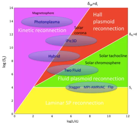
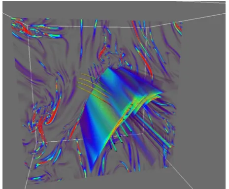
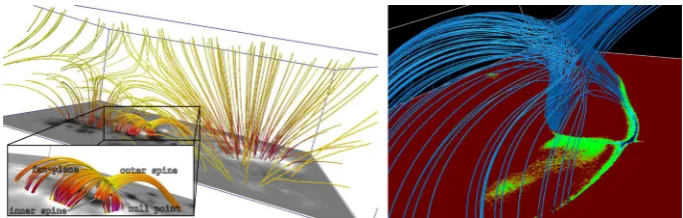
In order to study and understand these multi-scale physics processes of fundamental importance for Space Weather model-ling, one possibility is to make use of a full kinetic model, as with PIC or Vlasov numerical codes. However, these codes are still today out of the available computational power even when using massively parallel machines. This is why to describe this multi-scale physics all together is today one of the major challenges in plasma physics that requires the cou-pling of different models, from fluid to kinetic. As it is well-known, each of these approaches is most suitable for specific plasma regimes and/or to treat specific plasma processes. The SWIFF framework aims at coupling them across an interface or overlapping region, as illustrated in Figure 4 for the case of magnetic reconnection in the Earth’s magnetotail.

Previous works have focused on the coupling between MHD and the PIC codes Sugiyama et al. (2006), Sugiyama & Kusano (2007). However, the MHD approximation is a con-sistent model only at very large fluid scales, much larger than the ion inertial length and/or the ion Larmor radii,L» di,qi.

This is why kinetic codes also have to run using ‘‘large’’, fluid domains to efficiently communicate with MHD codes and, any-way, the physical gap between MHD and full kinetic models appears too large. In other words, the coupling between MHD and PIC codes appears not optimal from a physical point of view and is still out of reach on nowadays computational

resources in 3D geometries. An efficient way to overcome this problem of coupling a large-scale fluid code (e.g., a MHD code) and a kinetic code (e.g., a PIC code) requires to take into account an intermediate level of modelization that fills the gap between MHD and kinetic models. To increase the degree of realism and our understanding of the physics at play in regions of transition between fluid and kinetic behaviour, one needs to include both two-fluid effects and the most relevant kinetic processes in the model. This second point can still be achieved in a fluid framework. Efforts have been done both from theoretical and computational points of view to include dominant kinetic corrections, as including finite Larmor radius effects in the pressure tensor or linear Landau damping in the heat flux equation, still in the framework of fluid modelling

Sulem & Passot (2008).

2.4. Summary of codes available in SWIFF

The SWIFF approach combines multiple physical models: from a single fluid MHD, to Hall MHD, two-fluid MHD, advanced fluid models that include kinetic aspects, hybrid fluid-kinetic methods and fully kinetic methods. Table 1 lists numerical codes developed and being used by the member institutions of SWIFF consortium. Each of these approaches is most suit-able in specific regions to treat specific processes and the SWIFF framework aims at coupling them across an interface or on overlapping regions, as illustrated inFigure 4.

3. First SWIFF application: magnetic reconnection

The major application for the multi-scale simulation tool is to address magnetic reconnection, going beyond the detailed inter-code comparisons in the context of the well-documented Geo-space Environmental Modeling (GEM)Birn et al. (2001)and NewtonBirn et al. (2005)challenges. The challenges are to revi-sit the many recent insights obtained by the various teams involved in this proposal, realizing both 2D and 3D multi-scale simulations in especially collisionless magnetic reconnection regimes. We intend to perform detailed simulations tailored to plasma configurations relevant for coronal mass ejections in the solar corona, heliospheric current sheet conditions and

magnetospheric reconnection sites. In all of these settings, the role of spatial shear flow combined with magnetic shear is to be explored in detail. Using the hybrid simulation suite, we aim to quantitatively address the role of incorporating ideal to Hall-MHD, single to multi-fluid, as well as fluid to kinetic aspects under realistic and reproducible initial and boundary conditions. A major challenge in modeling many space and laboratory reconnection events is to reproduce the observed (high) recon-nection rates. For this it is crucial to know if, at the small scales, the process is laminar or turbulent. At these small scales, fluid modeling has to be complemented with kinetic modeling of the charged particle velocity distributions. While the plasma fluid turbulence exhibits vortices and shear flows in 2D or 3D, the energy-dependent particle trajectories in the kinetic model effectively extend the turbulent fluctuations to a higher-dimen-sional phase space, which may lead to enhanced reconnection or to collisionless damping due to phase space mixing. Using the many (hybrid, PIC and grid-adaptive) codes that SWIFF jointly shares, we performed a first detailed comparison of the different algorithmic approaches within the first half year of our efforts and swiftly move on to develop and integrate this knowledge in the targeted multi-scale approach.

3.1. Reconnection as a multi-physics challenge

The current understanding of reconnection identifies different types of reconnection depending on the parameters of the physics problem.Figure 4summarizes the different regimes in a diagram of the Lundquist number SL=l0LVA/g versus the

thickness of the reconnecting layer normalized to the ion inertial lengthdi=L/di(Ji & Daughton 2011;Baalrud et al. 2011):

– At the smallest scales, when ion inertial lengthdiis bigger

than the current sheet thickness predicted by Sweet-Parker model dSP= LSL1/2 (upper left of the diagram), the kinetic regime of fast reconnection develops leading to the formation of a single dominant X-point where a two scale process develops with an outer ion diffusion region where the ions become decoupled from the field lines and an inner electron diffusion region where also the elec-trons become decoupled. To capture this regime of recon-nection, simple one fluid models (of the MHD type, used in the present benchmark) cannot be used. At a minimum Hall or electron MHD need to be used. Two-fluid, hybrid code and kinetic codes can of course capture this regime. – At the largest scale, the single fluid MHD description is valid, and two-fluid regimes of reconnection are possible: the Sweet-Parker slow regime and the turbulent fast regime characterized by secondary plasmoids (lower right of the diagram). The transition between the two regimes has been shown to happen at a critical value of the Lundquist num-berSC= 104(Skender & Lapenta 2010).

– At intermediate scales when dPL<di<dSP, where the

resistive skin depth for plasmoid dPL= dSP(VA/L/c)1/2,

and cis plasmoid growth rate, an intermediate regime is present where secondary plasmoids are formed even though the ion-electron separation of scales is present.

3.2. Reconnection as a multi-scale challenge: Turbulent Reconnection

The multi-scale aspect of magnetic reconnection comes naturally into focus when dealing with reconnection in the solar

corona, where the span from macroscales (tens of thousands of km) to microscales (mm to cm) is huge, and cannot possibly be bridged directly by numerical simulation. The huge range of scales also implies that one cannot successfully ‘‘blame’’ fast reconnection on mechanisms operating at the microscale. What happens at the microscale is relevant to aspects such as particle acceleration and radiation signatures, but just as in hydrody-namic turbulence the cascade of energy from large scales to small scales operates essentially independent of details of what happens at the dissipation end of the cascade.

The fact that the rate of dissipation of large-scale kinetic energy in a turbulent hydrodynamic system does not depend on details of dissipation at the microscale has been understood and accepted since the early work byKolmogorov (1941). The scaling of the dissipation rate is given by the expression

_

Ekin Cq0U 3

rms=L; ð1Þ

where q0 is the mean mass density, Urms is the root-mean-square turbulent velocity, L is the size of the system and C is theKolmogorov constant; a constant of the order of unity.

Equation (1) has the simple interpretation that the kinetic energy q0U2rms/2 decays in a time similar to the turbulent turn-over time L/Urms.

In the context of interstellar medium turbulence it was ini-tially thought, based on arguments related to the slow decay of torsional Alfve´n waves, that magnetohydrodynamic turbulence would decay on a much longer time scale. However, numerical experiments showed this not to be the case, and similar results obtained by several groups (Mac Low et al. 1998;Stone et al. 1998; Padoan & Nordlund 1999) confirmed that the energy decay rate of magnetohydrodynamic turbulence obeys a similar scaling law as the one for hydrodynamic turbulence, differing only in that the energy involved is the sum of the turbulent kinetic and magnetic energies.

Kritsuk et al. (2011) compared the results on decaying supersonic MHD-turbulence from a large number of codes and found that the energy decay rate was indeed one of the most robust results, for which all codes gave essentially the same results.

For historical reasons the topic of magnetic reconnection developed along different lines, with a long-lasting focus on the dissipation in single, monolithic current sheets, separating two regions with totally smooth and well-ordered fields, with the Sweet-Parker current sheet (Parker 1957; Sweet 1958) as the archetype setup, and emphasizing the question of how to achieve sufficiently fast reconnection in similar arrangements.

In the specific context of solar corona heating,Parker (1972,

1983a,b,1987,1988) suggested that braiding motions from the sub-photospheric layers would inevitably, in a finite time, lead to the formation of a complex structure of electric current sheets (discontinuities in the magnetic field direction), whose total dis-sipation could be estimated by balancing the disdis-sipation against the corresponding work that would have to be done at the photo-spheric boundary (Parker 1988). The formation of (mathemati-cal) current sheets in a finite time was questioned by van Ballegooijen (1985,1986), who argued that the electric current density would remain continuous, for continuous boundary motions. The predicted scaling of the magnetic energy dissipa-tion rate was, for practical purposes, the same in the two theo-ries, with the angle of inclination of magnetic field lines at the driving boundaries as the main unknown factor.

Strauss 1991;Gomez & Ferro Fontan 1992;Longcope & Sudan 1994;Galsgaard & Nordlund 1996). The results could be seen as vindications of both points of view: the electric current density in principle remained smooth, but for any given, limited numerical resolution the current density structures in practice became indis-tinguishable from numerical representations of mathematical cur-rent sheets. As anticipated by both Parker and van Ballegooijen high magnetic Reynolds number magnetic dissipation takes place in complex, hierarchical structures of current sheets (see e.g.,Galsgaard & Nordlund 1996;Figs. 5and7here).Galsgaard & Nordlund (1996, 1997), Nordlund & Galsgaard (1997)

showed that the angle of inclination of magnetic field lines at the driving boundaries could be estimated by observing that the winding numberof magnetic field lines, as they pass from one boundary to another, cannot easily exceed unity, and hence arrived at a scaling formula for magnetic dissipation of the type:

_

Emag CmagB20Udriveðl=LÞ=L; ð2Þ

whereB0is the mean magnetic field,Udriveis the amplitude of the driving motion at the boundary,Lis the size of the system along magnetic field lines, and the factor‘/Lis the ratio of the correlation length ‘of the driving motion to the lengthLof magnetic field lines, thus expressing the dependence on the angle of inclination at the boundaries on the winding of magnetic field lines.

NeitherEq. (2)nor the corresponding estimates of the mag-netic dissipation rates in Parker (1988) and van Ballegooijen (1986)depend on the electric resistivity; that dependence drops out because the magnetic field is forced to develop structure at the smallest scales to an extent that allows the magnetic dissi-pation to balance the work done at the boundaries.

Lazarian & Vishniac (1999) and coworkers (Cho et al. 2002,2003;Eyink et al. 2011;Lazarian et al. 2012) have since returned to the question of magnetic dissipation in Sweet-Parker-like current sheets, and have shown that an externally imposed turbulent velocity field leads to an enhanced magnetic dissipation rate that also does not depend on the electric resis-tivity. Under the assumption of externally imposed turbulence the reconnection rate does of course depend on the magnitude of that turbulence, with a reconnection speed scaling as

Vrec lP1=2; ð3Þ

where‘is now the injection scale for turbulence andPis the power of the injected turbulence.

As emphasized e.g. by Lapenta & Bettarini (2011) and

Lapenta & Lazarian (2012), one may expect that in sufficiently high-resolution numerical simulations turbulence will be self-consistently generated, with the ‘‘exhaust flow’’ from each cur-rent sheet interacting with and creating new turbulent structures and new current sheets. Such a state of affairs may be thought of as approaching the generic MHD-turbulence modelled by

Mac Low et al. (1998)and others (Stone et al. 1998;Padoan & Nordlund 1999) or, in the case of boundary driven reconnec-tion, the type of current sheet hierarchy modelled by Mikic et al. (1989)and byGalsgaard & Nordlund (1996).

Reconnection in realistic systems, such as for example in models of the solar corona, may give rise to situations where the overall topology of the magnetic field defines local regions of interest (null points, nearly reversing magnetic fields, etc.), surrounded by relatively large regions of lesser interest. With Adaptive Mesh Refinement techniques one may then zoom in on specifically the region(s) of interest, while leaving the

peripheral regions more moderately resolved. Whether Adap-tive Mesh Refinement can be used with significant advantage in the reconnection region itself is more doubtful, since uni-grid studies tend to show rather closely packed current sheet struc-tures, particularly when low amplitude electric current sheets, which may nevertheless be an important factor, are considered.

4. SWIFF approach to the reconnection challenge

4.1. Simulation setup

The problem was simulated in two-dimensional plane only in the initial comparative study. The physical size of the system in each direction is labelled asLx and Lz. The initial state of

the Harris equilibrium is characterized by a balance of magnetic and plasma pressures. Plasma pressure is:

p zð Þ ¼ p_bþ B 2 0 2 cosh

2 z

L ; ð4Þ

with background pressurepb¼B

2

0=20. Equilibrium magnetic field can be written asB= (Bx,0,0) where

Bxð Þ ¼z B0tanh z

L : ð5Þ

Spatial scales are normalized with respect to the characteristic scale of the Harris sheet, so thatL= 1. Magnetic field is nor-malized with respect to peak magnetic field, i.e.,B0= 1. Resis-tivityg is set by the value of Lundquist numberS=l0LVA/g which is chosen to be equal to critical value of Lundquist

number S =Sc= 104 for transition between Sweet-Parker reconnection regime and fast turbulent regime (see Fig. 4). Viscosity l is set by the value of Reynolds number R=LVA/L= 10

4

, hereVAis the Alfve´n velocity,VA= 1 in sim-ulation units. The system is initialized with a small-amplitude perturbation of the magnetic vector potential which initiates the formation of the current sheet. The problem was tested in two configurations, in the first case, the simulation domain contains single Harris sheet and the size of the physical box isLx/L= 240 andLz/L= 60. In the second case, the simulation

domain contains two sheets (located at z= 0.25 Lz and

z= 0.75Lz) and the size of the physical box is Lx/L=

Lz/L= 30.

4.2. Intracode comparison

Figure 6compares reconnected fluxes (quantified by the differ-ence between maximal and minimal values of out-of-plane component of vector potential along the original current sheet location) and corresponding reconnection rates obtained in var-ious numerical codes. The typical evolution of the reconnection process is characterized by the reconnected flux. This is the amount of magnetic flux gone through the process of reconnec-tion. Its time derivative, the reconnection rate, is one of the most important parameters in determining the scale of energy release during space weather processes. For example, it impacts the rate of CME detachment from the corona and the speed of energy release during flux transfer events in the magnetosphere. It is then one of the most important parameters to compare in code comparisons.

Transition between laminar Sweet-Parker reconnection and fluid plasmoid reconnection is observed in MHD runs. This phenomenon is illustrated in Figure 7 which shows state of the evolution of FlipMHD simulation of single layer setup (Lx/L= 240) at two times. Left panel shows the early

Sweet-Parker phase with just one very elongated central current sheet. Right panel shows mature phase with multiple magnetic islands. During this phase, the reconnection is fast and turbu-lent. This behaviour was previously reported by Lapenta (2008), Uzdensky et al. (2010), Lapenta & Lazarian (2012). During the Sweet-Parker phase, only one island is present in the system. The current sheet breaks into two and new magnetic island appears approximately at t= 320tA. The two new

current sheets break later also and two more magnetic islands appear approximately at t= 360 tA. Obviously, the transition between the Sweet-Parker regime and plasmoid regime is char-acterized by an increase of reconnection rate, see the black curve inFigure 6.

Similar behaviour is observed also in hybrid model for the single layer setup with bigger system size (Lx/L= 240).

How-ever, in agreement with current understanding of reconnection process, this behaviour changes when the system size is decreased. In the case of double layer setup with system size Lx/L= 30, singleX-point reconnection is observed. This

differ-ence is illustrated in Figure 8, where snapshots from hybrid simulations withLx/L= 240 andLx/L= 30 are shown.

The onset of magnetic reconnection is a complicated phys-ical problem, since multiple instabilities can trigger it. The time when the reconnection sets up in the simulation depends on the physical model employed by the numerical code. In general, it is faster in kinetic and hybrid models, where more plasma insta-bilities are at play. Our code comparison, in agreement with the results of GEM challenge Birn et al. (2001), suggests that reconnection starts faster and the reconnection rate is higher, in the simulations of Hybrid and iPic3D codes (Fig. 6). While the reconnection onset times are longer, reconnection rates are lower in the MHD runs. It is worth to add, that in the latter sim-ulations the reconnection rate highly depends on the imposed viscosity (diffusivity) and grid resolution.

The reconnection challenge performed within the SWIFF project so far demonstrates variability of reconnection regimes occurring under different conditions and in different simulation models. At small scales the single fluid MHD picture is valid only if enough resolution is used so that the secondary plasm-oids are resolved and the onset of the fast turbulent phase of reconnection is captured. This description is adequate for the modelling of reconnection in the base of the solar atmosphere. However, in the solar corona and in the Earth magnetosphere, reconnection is dominated by the separation of electron and ion scales leading to a strong Hall effect and differential motion of ions and electrons. To capture this regime of reconnection, improved fluid models, hybrid or kinetic codes are needed. The combined use of the codes possessed by member institu-tions of SWIFF consortium is able to capture all required regimes and describe all physical systems of interest for space weather.

5. Observational validation of reconnection results

One of the most important consequences of post-CME mag-netic reconnection is the formation of post-CME Current Sheets (CS). Observationally, these features have been identified in white light data acquired by SOHO/LASCO and STEREO/ COR coronagraphs (Webb et al. 2003;Patsourakos & Vourlidas 2011) as radial long-lived features observed coaligned with the CME, and in principle their detection is possible also in the STEREO/HI heliospheric imagers. Moreover, over the last dec-ade post-CME CS have been identified in UV spectroscopic data acquired by SOHO/UVCS (Solar and Heliospheric Obser-vatory/UltraViolet Coronagraph Spectrometer), typically detected as strong brightening in UVCS spectra in the FeXVIII 974A˚ spectral line (Ko et al. 2003; Ciaravella & Raymond 2008). This spectral line forms at a very high plasma tempera-ture, around 5 MK, quite high even for the ‘‘hot’’ solar corona. The origin of this very high temperature plasma is an open issue: it could originate for instance from turbulent reconnection occurring in the post-CME CS (Bemporad 2008), or alterna-tively from Petschek reconnection occurring at the base of it, in correspondence of the location of the post-flare Hard X-ray (HXR) source (Saint-Hilaire et al. 2009). In particular, the ther-mal energy content of the HXR source observed by RHESSI could be even much larger than the energy required for the

post-CME CS plasma heating as observed higher up by UVCS, but the X-ray source decays typically in a few hours after the eruption, while the high-temperature emission observed by UVCS lasts for more than 2 days after the CME. Hence, Petschek reconnection at the base of the CS seems to be respon-sible for the observed plasma heating only in the early phases of the post-CME coronal reconfiguration.

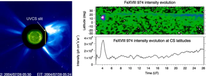
For the purposes of the SWIFF project we selected two interesting limb events detected by UVCS which occurred on November 2, 2003 and on July 28, 2004. From the UV and white light remote-sensing data we plan to estimate: CS thick-ness and length (directly observed; WL and UV), density (col-umn density; WL and line ratio; UV), thermal energy content (UV lines; UV), turbulence velocity (line non-thermal broaden-ing; UV), density time fluctuations (intensity fluctuations; WL), Alfve´n velocity (from propagating blob velocities; WL). Remote-sensing data will be also complemented with in situ observations: CS are observable in the interplanetary medium by in situ data, looking at the current density as the spacecraft crosses the sheet. In situ data can be used to derive: CS thick-ness, density, density fluctuations, Alfve´n velocity. Preliminary analysis of the July 28, 2004 event shows the detection by UVCS of a first short-lived (~1 h) bright peak in the FeXVIII 974 A˚ line intensity, observed ~30 min after the CME,

Fig. 9. Left panel: composite LASCO/C2 and EIT 195 A˚ images acquired on July 28, 2004 at 05:30 and 05:24 UT, respectively. The solid yellow line shows the location of the UVCS slit field of view centred 0.8 solar radii above the West limb.Right panel: the evolution of FeXVIII 974 A˚ line intensity observed by UVCS after the July 28, 2004 CME at different latitudes (top panel) and averaged over the CS latitudes (bottom panel).

followed by a slow (~20 h) gradual FeXVIII 974 A˚ line inten-sity increase (see Fig. 9). The persisting and gradually rising FeXVIII emission was detected by UVCS 0.8 solar radii above the limb and was associated also with a persisting Hard X-ray and Soft X-ray source on disk at the top of the post-flare loops, as observed by RHESSI and GOES/SXI instruments, respec-tively. From the electron temperature and densities measured by UVCS in the post-CME CS with line ratio technique we will estimate the total CS thermal energy and compare it with that provided by the X-ray sources at the base of the CS. These observations are now being compared with simulations performed within the SWIFF Project. The CS temperatures provided by MHD simulations cannot be trusted, because a polytropic relation is used for the low corona, which gives not fully reliable temperatures. In particular, temperatures from full MHD simulations turn out to be much smaller than the high temperatures (5 MK) observed in UV (C. Jacobs, priv. commun.). Hence, we are now performing hybrid simulations of turbulent reconnection. The simulation is first performed in 2D in a ‘‘box’’ of size 104·104km2containing the CS and located in the altitude range between 1.5 and 2.5 solar radii. Boundary conditions are derived by assuming ‘‘realistic’’ (i.e., given by observations) coronal electron density ne, electron temperatureTeand magnetic fieldBradial profiles fromGibson

et al. (1999), Va´squez et al. (2003), Dulk & McLean (1978), respectively. For instance, at the heliocentric distance of 1.8 solar radii (where typically UVCS observed the post-CME CS evolution), the above profiles give ne= 4.3·106cm3, Te= 1.5·106K and B= 0.70 G, respectively. Starting from a CS region initially denser (by a factor ~10) and hotter (by a factor ~5) than the surrounding corona, the system is evolved in time allowing turbulent reconnection in the CS. The code simulates the evolution of kinetic temperature of three species: electrons, protons and a heavy ion. In particular, in order to compare simulation results with observations by UVCS, the heavy ion is selected with a charge-to-mass ratio equivalent to that of the ion Fe+17responsible for the FeXVIII 974 A˚ line emission.

6. Application of the SWIFF modelling approach to space weather problems

6.1. Coupling at the Sun

Solar activity events, precursors of space weather, are produced by magnetic field emergence and evolution in the Sun. Our pri-mary goal is to produce models of these events based on both observed (extrapolated) and simulated configurations of mag-netic fields. Active region scale structures are created spontane-ously by the hierarchy of (magneto-)convective sub-surface flows. A uniform horizontal magnetic field fed into the bottom boundary of a magneto convection model is massaged by the convective flows into loop-like structures, as illustrated by

Figure 10.

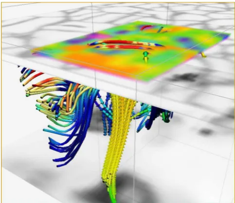
Above the solar surface the magnetic field dominates the dynamics, with magnetic energy flowing into the corona (upward directed Poynting flux) due to both new magnetic flux emerging through the solar photosphere and due to stretching and twisting of the coronal magnetic field by horizontal motions.Figure 11shows a snapshot of such a dynamic mag-netic field, with stress being added particularly as a result of the spinning motion of the small sunspot in the lower left hand cor-ner of the figure (Fig. 12).

The dynamics in the corona is nearly collisionless and gives rise to nonthermal particle energy distributions, including high-energy power laws evidencing that particle acceleration occurs in the solar corona. To provide a background for understanding how such particle acceleration may come about combined MHD + particle-in-cell (PIC) models of an observed active region have been constructed Baumann & Nordlund (2012),

Baumann et al. (2012a,2012b).

Boundary conditions and initial magnetic field configura-tions are obviously required for MHD and particle models of CMEs, flares and the Sun’s global coronal field as a whole. In order to provide realistic conditions derived from observed magnetograms, a model which enables stresses within the mag-netic field to be built up over long periods (from days to months) is required. These stressed fields not only produce more realistic boundary conditions, but are also much more accurate in identifying regions from which CMEs and flares may be initiated. Additionally, they provide a realistic starting point for more detailed small-scale models involving additional physics.

The basic nonlinear global field model couples the surface flux transport modelYeates et al. (2007) with the quasi-static coronal evolution model of Mackay & van Ballegooijen (2006)and Yeates et al. (2008). The observed magnetic field of newly emerged bipoles taken from observed magnetogram data is evolved taking into account large-scale flows due to dif-ferential rotation and meridional flows, supergranulation and the cancellation of flux to produce a continuous evolution of the magnetic field and current density in the photosphere. The resulting magnetic field compares well with observed syn-optic magnetograms and provides a boundary condition that evolves following appropriate physical rules. In the coronal evolution model, the magnetic field within the volume is evolved via the ideal induction equation in response to the

boundary motions. To ensure the coronal plasma evolves though a series of force-free states, a magnetofrictional method is utilized. A continuous sequence of nonlinear force-free fields is then formed in response to the observed photospheric motions and emerged flux. This coupled model enables the long-term continuous build-up of free magnetic energy and electric currents in the corona to be followed. Not surprisingly, the structure and behaviour of the magnetic fields formed differ significantly from those found from extrapolation approaches which retain no memory of magnetic flux or connectivity from one extrapolation to the next.

Of particular interest to SWIFF is the development of suit-able magnetic field structures with configurations for flares and CMEs which are known in many cases to be associated with prominences/filaments. Thus the above magnetofrictional model has been improved to provide much better models of prominences/filaments. The magnetofrictional model has been shown to model the chirality (the handedness of twist) of filaments well in many, but not all, cases. Indeed, it has a 96% success rate for filaments in active region latitudes, i.e., below 60latitudeYeates et al. (2007,2008),Yeates & Mackay (2009). However, since around half of all CMEs originate from outside active regions, it is important to be able to properly model the chirality of high-latitude filaments. When injecting new bipoles (active regions) into the surface flux transport model, a net helicity of a particular sign is included for each

active region according to whether it emerges in the northern or southern hemisphere. This large-scale helicity term is impor-tant in creating the correct chirality of low-latitude filaments. However, this helicity may be lost through eruptions and so does not get carried to high latitudes. Our current work involves injecting additional helicity at small scales. In order to obtain the correct chirality of filaments at high latitudes, it has been found that injecting helicity at small scales via an additional term in the induction equation of the magnetofrictional code significantly helps.

6.2. Coupling at the magnetosphere

The solar wind-magnetosphere coupling plays a key role in the context of space weather modelling and forecasting. This cou-pling strongly depends on the solar wind properties and their variability. The connection between the solar wind and magne-tosphere is mediated through the magnetosheath and magneto-pause boundaries. From a theoretical/modelling point of view, the solar wind-Earth’s magnetosphere environment is also a lab-oratory of excellence to study the physics of several fundamen-tal processes that play a key role in the context of space weather. The great interest in the analysis of these processes is first, because of their importance in the shaping and dynamics of the solar wind – Earth’s magnetosphere region and second, because of the wealth of in situ diagnostics of improving quality

Fig. 11. Left panel: Snapshot of the coronal magnetic field in a model where the coronal dynamics and heating is studied in the MHD approximation, with driving (as well as sunspots) supplied ab initio by the sub-photospheric part of the model.Right panel: the corresponding chromospheric (dark) and coronal (yellow and red) temperature structure. Red indicates temperatures in excess of 10 million K. The rotating sunspot at the lower left in the left-hand side panel is seen in front of the projected photospheric surface in the right-hand side panel. The simulation was performed with the Stagger code.

accumulating in the form of electromagnetic profiles and parti-cle distribution functions. Concerning the solar wind-magneto-sphere coupling at the flanks of the magnetowind-magneto-sphere, satellite measurements have supplied clear evidence of rolled-up vorti-ces at the flank of the Magnetopause Fairfield et al. (2000),

Hasegawa et al. (2004). In this region, the Kelvin-Helmholtz Instability (KHI), generated by the velocity shear between the magnetosheath and magnetosphere velocities, has been proved to play a crucial role in the interaction between the solar wind and the Earth’s magnetosphere and to provide a mechanism by which the solar wind enters the Earth’s magnetosphere. The understanding of the mechanisms responsible for the solar wind entering in the Earth’s magnetosphere is of great importance in the context of the physics of the magnetosphere and, as a con-sequence, for space weather phenomena such as magnetic storms and aurorae.

The KHI has been invoked as a possible mechanism to account for the increase of the plasma transport since during northward magnetic field periods, when magnetic reconnection is considered as inefficient, a relevant mixing between the solar wind and the magnetospheric plasma is observed, even larger than during southward configurations. KHI instability driven by a velocity shear can grow at low latitude since the nearly per-pendicular magnetic field does not inhibit instability develop-ments. This provides an efficient mechanism for the formation of a mixing layer and for the entry of the solar plasma into the magnetosphere, explaining the efficient transport during north-ward solar wind periods. Several observations support this explanation and show that the physical quantities observed along the magnetopause flank at low latitude are compatible with KH vortices Fairfield et al. (2000), Hasegawa et al. (2004). The velocity jump across the shear layer is roughly equal to the magnetosheath velocity (the magnetosphere plasma veloc-ity being much smaller), which is of the same order (a fraction smaller) as the free solar wind speed,DU400 km/sPetrinec et al. (1997). The KHI can be stabilized by two effects: compres-sion and magnetic tencompres-sion. First, in the case of a large sonic Mach number Ms= DU/cs> 2, where cs is the sound speed, the shear flow is able to generate KH vortices, but generates shocks or radiates compressional wavesMiura (1990). Note that the shocked magnetosheath plasma has a sonic Mach number smaller than 1. However, the magnetosheath plasma velocity is known to increase as it flows away from the shock along the magnetotail. This is why such stabilization should be of interest mainly downstream, along the magnetotail, while it should play a negligible role in the vicinity of the Earth. Second, in the presence of a magnetic field parallel to the flow, the KHI may be inhibited by the stabilizing magnetic tension. In this case, the critical sheared velocity for the development of rolled-up KH vortices is such that the ‘‘in-plane’’ Alfve´nic Mach number must be larger than 5Baty et al. (2003)(Ma=DU/va, where ua is the Alfve´n speed considering the component of the magnetic field in the KH-unstable plane). This is in general verified at the Magnetopause at low latitudes during northward solar wind magnetic field conditions, since the magnetic field is mostly perpendicular to the KH-unstable plane. Such a regime is well handled by the codeFaganello et al. (2008a).

The nonlinear evolution of the large-scale fluid vortices and/or the development of secondary instabilities, self-consis-tently cascade the energy towards smaller and smaller scales, where the dynamics become kinetic, playing a significant role in the transport properties of the global system. Figure 13

shows an example of secondary KH instability that generates small-scale vortices on the edge of a primary large MHD-scale

vortex. The vortex formation process drags the magnetic field component parallel to the solar wind direction into the flow. As a result, the magnetic field is thus more and more stretched inside the vortices until it reconnectsFaganello et al. (2008a,b),

Califano et al. (2009),Henri et al. (2012), redistributing the ini-tial kinetic energy into accelerated particles and heating. More-over, the density jump between the magnetosheath and magnetospheric plasmas drives fluid-like secondary instabilities such as the Rayleigh-Taylor instabilityFaganello et al. (2008c),

Tenerani et al. (2011). The density ratio between the magneto-sheath (10–100 cm3) and the outer magnetosphere (0.1– 10 cm3) plasmas is typically of the order of 10 Escoubet et al. (1997),Petrinec et al. (1997), on a few ion inertial lengths. The magnetosheath ion inertial length isdi~ 100 km.In these

conditions, the KHI rolled-up vortices generate gradients on length scales of the order of the ion inertial length across the vortex arms, leading to density gradients Dn/L ~ 0.1 – 1 cm3km1. Depending on the local plasma parameters, the density gradient can be considered critical when the RT instability growth rate becomes larger than both (i) the inverse time scale for vortex pairing and (ii) the growth rates of other secondary instabilities (secondary KH, VIR). On top of that, the downstream increase of the magnetosheath velocity leads to super-magnetosonic regimes for which the Kelvin-Helmholtz vortices act as obstacles to the plasma flow, generating quasi perpendicular shocksPalermo et al. (2011a,b), thus modifying the transport properties of the plasma of the solar wind-magne-tosphere. It is thus crucial to establish the role of these different secondary instabilities on the dynamics of the system, since they strongly influence the increase of the width of the mixing layer and its internal dynamics that are the most important fac-tors for the evolution at the flank of the Earth’s Magnetosphere. To summarize, the interaction of the solar wind with the Earth’s magnetosphere leads to a complex multi-scale dynamics where various instabilities, turbulence and other fundamental

processes, e.g., magnetic field reconnection, play a very impor-tant role. To progress beyond state of the art in this problem, the primary physical processes and kinetic effects at play should be understood through the complementary use of different models, from fluid to kinetic. In this context, we decided to start a benchmarking activity, the Magnetopause Challenge, that focused on the comparison between different codes/models of the development of the Kelvin-Helmholtz instability in a mag-netized plasma, starting from a sheared velocity configuration

Henri et al. (2013).

6.3. Coupling at the Earth

The solar wind variations have also an influence on the inner magnetosphere. In these magneto-spheric regions, the kinetic processes prevail so that the kinetic approach has been used in the model development. In the framework of SWIFF, kinetic models have been developed and improved for different regions of the magnetosphere: the plasmasphere Pierrard & Stegen (2008),Pierrard & Voiculescu (2011), the polar windPierrard & Borremans (2012a) and the radiation belts (Pierrard et al. 2012b). In addition, kinetic solar wind models have also been expanded and improved Pierrard (2011b), Pierrard et al. (2011), Pierrard (2012b) since the solar wind variations are directly related to magnetospheric perturbations.

In these kinetic models, the velocity distribution functions of the particles are determined by solving the evolution equationPierrard (2011a). The models predict physical param-eters of the particles such as their densities, flux, temperatures, heat flux as well as their boundaries like the plasmapause posi-tion in the case of the plasmaspheric model. The effects of suprathermal particles on the escape flux and the temperature profiles are specifically studiedPierrard (2012a).

The dynamics of the plasmasphere is mainly determined by the convection electric field combined with the corotation elec-tric field. The position of the plasmapause, the limit of the plasmasphere, is determined by the interchange instability mechanism and depends on the level of geomagnetic activity. During geomagnetic storms and disturbed periods, the plasma-sphere is eroded; a sharp plasmapause is then formed closer to the Earth in the post-midnight sector and a plume is later gen-erated in the afternoon MLT sector.

In the SWIFF project, the kinetic plasmasphere model has been coupled with the International Reference Ionosphere (IRI) model to determine the composition, the number density and the temperature of the different particles Pierrard & Voiculescu (2011). The ionosphere model is used at low alti-tudes as boundary conditions for the 3D time-dependent plasmasphere model. The highest densities are located in the ionosphere. Correspondence exists between the plasmapause position and the F region ionospheric trough. Coincident obser-vations of middle and top ionosphere, satellite tomography, radar measurements and plasmapause observations are used to investigate the conditions when the F region trough is asso-ciated with the plasmapause.

The ionosphere-plasmasphere coupled system is a highly dynamic region that presents different features depending on the geomagnetic activity. As illustrated inFigure 14, a plasma-spheric plume appears in the dusk sector after an increase of the geomagnetic activity. A grid of 300·180·180 points is used for the radial distances, magnetic longitude and latitude, respectively.

Dynamical simulations of the plasmasphere are provided on the space weather portal2for nowcasting or for forecasting at any other date given as an input. The dynamical simulations show equatorial and meridian views of the plasmasphere evolu-tion every half hour during one day.

At high latitudes, the ionospheric particles are not trapped in the plasmasphere but escape along the open magnetic field lines. The kinetic model developed for this polar wind escape

Pierrard & Borremans (2012a)is also provided on the space weather portal.

Finally, the energetic protons and electrons trapped in the magnetic field of the Earth have also crucial scientific and practical significance for space weather since they can harm space-borne systems and astronauts. The proton radiation belt comprises very energetic protons located close to the Earth. It is quite stable except at very low altitudes where the expansion of the atmosphere can erode it. In Pierrard & Borremans (2012b), the differential flux observed in space radiations has been related to the characteristics of the particle momentum distribution functions. In fitting flux spectra by a sum of Maxwellians or by power laws, the slope of the differential flux was associated with the characteristic energy of the distributions and the normalization constant is proportional to the density. This analysis provides a density-energy description of the radiation belts and information on the origin and mechanisms influencing the radiation populations.

The outer electron belt is also highly variable with space weather. During geomagnetic storms, the electron fluxes vary from several orders of magnitudes and the outer belt penetrates closer to the Earth. By analysing satellite observations, we are developing a dynamic model of the electron flux variations during magnetic stormsBenck et al. (2013). The links between

Fig. 14. Density of the electrons obtained with the ionosphere-plasmasphere coupled model in the geomagnetic equatorial plane (left panel) and in the meridian plane corresponding to 12:00 to 24:00 MLT (right panel) on 10 September 2005 at 0:00 UT. The geomagnetic activity level index Kp observed from 9 to 11 September 2005 is illustrated in the upper panel.

2