Double observer line transect methods : levels of independence

Double-Observer Line Transect Methods: Levels of Independence

Stephen T. Buckland,1,* Jeffrey L. Laake2 and David L. Borchers1

1_{Centre for Research into Ecological and Environmental Modelling, University of St}

Andrews, The Observatory, Buchanan Gardens, St Andrews, Fife KY16 9LZ, Scotland

2 _{National Marine Mammal Laboratory, Alaska Fisheries Science Center, NMFS, Seattle,}

WA 98115, USA

SUMMARY. Double-observer line transect methods are becoming increasingly

widespread, especially for the estimation of marine mammal abundance from aerial and

shipboard surveys when detection of animals on the line is uncertain. The resulting data

supplement conventional distance sampling data with two-sample mark-recapture data.

Like conventional mark-recapture data, these have inherent problems for estimating

abundance in the presence of heterogeneity. Unlike conventional mark-recapture

methods, line transect methods use knowledge of the distribution of a covariate which

affects detection probability (namely distance from the transect line) in inference. This

knowledge can be used to diagnose unmodelled heterogeneity in the mark-recapture

component of the data. By modelling the covariance in detection probabilities with

distance, we show how the estimation problem can be formulated in terms of different

levels of independence. At one extreme, full independence is assumed, as in the Petersen

estimator (which does not use distance data); at the other extreme, independence only

occurs in the limit as detection probability tends to one. Between the two extremes, there

is a range of models, including those currently in common use, which have intermediate

levels of independence. We show how this framework can be used to provide more

simulation, and by analysis of a dataset for which true abundance is known. We illustrate

the approach through analysis of minke whale sightings data from the North Sea and

adjacent waters.

KEY WORDS: Distance sampling; Double-observer methods; Full independence; Limiting

1. Introduction

Distance sampling (Buckland et al., 2001) is widely used for estimating animal

abundance. In line transect sampling, an observer travels along each of a number of

lines, laid out according to some randomised (usually systematic random) scheme, and

records each detected animal, together with its perpendicular distance from the line. One

of the key assumptions of the method is that animals on the line are certain to be detected.

A number of authors have considered so-called observer or

double-platform methods to extend line transect sampling to the case that not all animals on the

line are detected (e.g., Buckland and Turnock, 1992; Palka, 1995; Alpizar-Jara and

Pollock, 1996; Manly et al., 1996; Quang and Becker, 1997; Chen, 2000; Innes et al.,

2002). The double-observer data can be regarded as two-sample mark-recapture.

However, heterogeneity in detection probabilities generates bias in abundance estimates,

just as heterogeneity in capture probabilities generates bias in mark-recapture estimates

of abundance. Authors have attempted to minimize this bias, for example by modelling

the effects of covariates (Borchers et al., 1998a,b; Borchers, 1999; Schweder et al.,

1999; Laake and Borchers, 2004; Borchers et al., 2006), or by assuming independence

in the detections of instantaneous cues (such as whale blows) rather than of animals

(Skaug and Schweder, 1999; Schweder et al., 1999).

In the absence of any heterogeneity in detection probabilities, we might assume

that observer j detects any given animal in the surveyed strip with probability ,

, and that the probability that both observers detect a given animal is .

This is the ‘full independence’ assumption. However, in line transect sampling, we allow

detection probability to fall off with distance y from the line so that . Thus it

is natural to apply the full independence assumption at each distance from the line, so that

for an animal at y, we assume

j p

2 , 1

=

j p₁₂ = p₁p₂

) (y p p_j = _j

) ( ) ( )

( 1 2

12 y p y p y

Laake (1999) introduced the concept of ‘point independence’ to reduce the impact

of unmodelled heterogeneity in detection probabilities. Knowledge of the distribution of

distances allows the full independence assumption to be weakened, as outlined below.

(For the moment, we ignore variables other than distance for simplicity.)

A double-observer line transect survey generates both conventional distance

sampling data and mark-recapture data. Under the assumption of uniform animal

distribution perpendicular to the transect line (achievable by random line placement or

systematic placement with a random start), the shape of the probability density function

of observed distances is the same as that of the detection function (Buckland et al.,

2001:52-53). The mark-recapture data provide additional information on the shape of the

detection function based on an assumption of independence of detection probabilities

without any assumption about the distribution of perpendicular distances of animals. If

we retain the assumption of uniform perpendicular distance distribution, discrepancies

between the shapes can be interpreted as failure of the assumption of independence

between detection probabilities.

We diagnose dependence by (a) modelling the shape of observer j’s detection

function ( , ) under the uniform perpendicular distance assumption, (b)

modelling the conditional probability that observer j detects an animal at y,

given that observer detected it ( )

(y

p_j j=1,2

) ( ' | y

p_{j j}

'

j j=1,2,j'=3− j) and (c) modelling the covariance in

the observers’ detection probabilities as a function of y using a function δ(y) defined

below.

For real data, typically does not decline as steeply as . Hence

the full independence assumption ( = ) cannot be made at each distance.

The reason for this is that at greater distances, only the most detectable animals tend to be

recorded, and those that are detected by one observer are therefore more likely to be )

( ' | y

p_{j j} p_j(y)

) ( ' | y

detected by the other observer. Laake (1999) argued that heterogeneity is less of a

problem on the line, where probability of detection is relatively high, than away from the

line, so that assuming independence only on the line should yield less biased estimates of

abundance. The idea was further developed by Laake and Borchers (2004) and Borchers

et al. (2006).

Although we can anticipate less dependence between detections on the line than at

greater distances, unless detection on the line is certain, it seems possible that some

dependence remains. In this paper, we consider levels of independence, and show that

the independence assumption can be weakened further by assuming that, as detection

probability tends to unity, dependence tends to zero (i.e., independence). We term this

‘limiting independence’.

We illustrate the methods through analyses of data from a shipboard survey of

minke whales in the North Sea and adjacent waters.

2. Methods

Suppose detected animals within a strip extending a distance W either side of the line are

recorded. We assume that two observers search independently from the same platform,

or from two platforms following the same route at almost the same time. We also assume

that duplicate detections can be correctly classified, based on time and location of

animals or animal cues, for example.

2.1 Independence Assumptions

At the simplest level, we might assume that observer 1 detects animals in this covered

strip with probability , while observer 2 independently detects animals with probability

. In this ‘full independence’ case, an animal is detected by at least one observer with

probability . A Horvitz-Thompson estimator of , the number of 1

p

2 p

2 1 2 1 p p p p

animals in the strip, is thus

∑

Nˆ_c 1 where is the number of animals detected

by at least one observer. Note that

n

12 2 1 n n n

n= + − where is the number of animals

detected by observer j, , and is the number of animals detected by both

observers. If we estimate by

j n 2 , 1 =

j n12

j

p pˆ_j =n₁₂/n_j' for j=1,2,j'=3− j, and substitute in, we

find that 12 2 1 ˆ n n n

N_c = , which is the familiar Petersen estimator. This is the full maximum

likelihood estimator of (Borchers et al., 2002:111), or within a single animal of the

maximum likelihood estimator, if we allow for the fact that is integer.

c N

c N

Now suppose that probability of detection is a function of distance y from the line.

There may also be dependence on additional covariates z, although we omit this

dependence below, for clarity. Full independence applied at each y gives

, so that a model is now needed for ,

) ( ) ( ) ( ) ( )

(y p1 y p2 y p1 y p2 y

p_• = + − p_j(y) j=1,2.

We can then proceed to fit the model, and hence to estimate abundance in the covered

strip (below).

We would like to relax the full independence assumption. Allowing some degree

of dependence (δ(y)), the independence assumption can be expressed more generally

such that p12(y)=δ(y)p1(y)p2(y), p•(y)= p1(y)+ p2(y)−δ(y)p1(y)p2(y), and

) ( ) ( ) ( '

| y y p y

p_{j j} = δ _j , j=1,2,j'=3− j. The function δ(y) is related to the

covariance σ12(y) between detection probabilities p1(y) and p2(y) as follows:

) ( ) ( ] 1 ) ( [ )

( 1 2

12 y = δ y − p y p y

σ . Various alternative expressions can be derived for δ(y)

including ) ( / ) ( ) ( / )} ( ) ( ) ( ) ( { )} ( ) ( /{ ) ( )

(y = p₁₂ y p₁ y p₂ y = p_1|2 y + p_2|1 y − p_1|2 y p_2|1 y p_• y = p_j|j' y p_j y δ

between the conditional detection functions derived from the mark-recapture

data and the unconditional detection functions which are derived from distance

sampling data with the requirement that is known for some . For distance

sampling with a single observer, the standard assumption is . With double

observers, this often untenable assumption can be replaced with the assumption of full

independence,

) ( ' | y

p_jj

) (y p_j

) (_y*

p_{j y}*

1 ) 0 ( = j p 1 ) (y =

δ for all y, or point independence, δ(y*)=1 at a specified ,

usually (Laake and Borchers, 2004). Fitting full independence models to data

requires a functional form for and point independence requires the same and a

model for . Neither require a model for

* y 0 *= y ) (y p_j ) ( ' | y

p_{j j} δ(y).

We now relax the assumption that δ(y*)=1 at a specified . Instead we

assume that we achieve independence in the limit as detection probability tends to one.

This requires a model for

*

y

) (y

δ with the following properties to ensure valid

probabilities:

1) δ(y)≤U(y) where U(y)=min

{

}

. 1 ) ( ' | y ≤

p_jj

2) δ(y)≥L(y) where

⎭ ⎬ ⎫ ⎩ ⎨ ⎧ + − = ) ( ) ( 1 ) ( ) ( , 0 max ) ( 2 1 2 1 y p y p y p y p y

L , which ensures that

. 1 ) ( ≤ • y p

If we defineδ₀(y)=

{

}

can be represented by an appropriate functional form such as a logistic. Note also that

Using a logistic formulation forδ₀(y), we can write ⎭ ⎬ ⎫ ⎩ ⎨ ⎧ − ( ) 1 ) ( log 0 0 y y e _δ δ as some

linear function of . Full and point independence can be derived as special cases of the

limiting independence model if we include the following offset

y ⎭ ⎬ ⎫ ⎩ ⎨ ⎧ − − 1 ) ( ) ( 1 log y U y L

e in δ0(y)

which fixes δ(y)=1. If we consider the following logistic model for limiting

independence: ⎭ ⎬ ⎫ ⎩ ⎨ ⎧ − − + + = ⎭ ⎬ ⎫ ⎩ ⎨ ⎧

− ( ) 1

) ( 1 log ) ( 1 ) ( log 0 0 y U y L y y y e

e _δ α β

δ

, (1)

then α =0 specifies point independence at y*=0, and α =β =0 specifies a full

independence model. If β =0 and α ≠0, a model with constant dependence for all

can be specified. Models restricted to independence or positive dependence can be

achieved by restricting

y

0 ,

0 ≥

≥ β

α . Hence this general formulation provides a model

selection framework for a range of models with varying degrees of independence.

2.2 Likelihood

The full likelihood for double-platform data may be expressed as L=LnLzLy|zL_ω where

is the component accounting for variation in total number of animals n detected by at

least one observer, corresponds to any observation-specific covariates

n L

z

L z,

corresponds to the conditional distribution of distances y, given covariates

z y|

L

z, and

corresponds to the mark-recapture data (Laake and Borchers, 2004). incorporates

the assumption of uniform distribution of animals perpendicular to transect lines. We use

just two components of the full likelihood: and . By doing this, we can avoid

making distributional assumptions about n and

ω L z y| L z y|

L L_ω

such assumptions. Instead, we draw inference conditional on n and z, and use a

design-based approach to allow for variation in n. If there are no covariates z, the full

likelihood is , and we use the second and third components only (in this case,

incorporates the assumption of uniform distribution of animals perpendicular to

transect lines). Again for simplicity we consider this latter case; the extensions to

include covariates ω

L L L

L= n y

y L

z are straightforward.

We have

∏

∏

1 1 ( )

) ( ) ( ) ( π L

where is the pdf of detection distances of animals detected by at least one

observer, evaluated at , )

(y_i

f_• y

i

y p_•(y_i)= p₁(y_i)+ p₂(y_i)−δ(y_i)p₁(y_i)p₂(y_i) is the probability

that an animal at distance from the line is detected by at least one observer, y_i π(y_i) is

the unconditional pdf of distances y in the population (whether detected or not), evaluated

at , and (Laake and Borchers, 2004:114). Random

positioning of the lines (or of a systematic grid of lines) ensures that

i

y E p_• =

∫

0 ( ) ( )

)

( π

W y) 1/

( =

π .

We also need

∏

1 ( )

) | Pr(ω ω L where )} ( ) ( 1 ){ ( } | ) 0 , 1 (

Pr{ω_i = y_i = p₁ y_i − p₂ y_i δ y_i

)} ( ) ( 1 ){ ( } | ) 1 , 0 (

Pr{ω_i = y_i = p₂ y_i − p₁ y_i δ y_i

) ( ) ( ) ( } | ) 1 , 1 (

Pr{ω_i = y_i = p₁ y_i p₂ y_i δ y_i

The likelihoods for full, point and limiting independence only differ in the definition of

) (y_i

use (Borchers et al., 1998b) and with the point independence assumption, and

can be maximized independently using models for and which separate

into the two respective likelihood components (Borchers et al., 2006). When the

likelihood is specified in terms of models for and ω

L L_ω Ly

) ( ' | y

p_jj p_j(y)

) (y

p_j δ(y), both components of the

likelihood must be maximized jointly.

We assume logistic forms for the detection functions:

) exp(

1

) exp(

) (

1 0

1 0

y y y

p

j j

j j

j _{λ λ}

λ λ

+ +

+

= for j=1 or 2. (2)

2.3 Diagnostic for Reliable Estimation under Limiting Independence

When fitting limiting independence models, the Hessian matrix is sometimes nearly

singular, due to high correlation between the estimates of p_j(y) and δ(y) at . In

these cases, the models are unstable, typically yielding very large abundance estimates

and associated variances. We can still usefully calculate Akaike’s Information Criterion

(AIC), but if AIC indicates that a limiting independence model is required, then reliable

estimation is not possible. To identify such cases, the following diagnostic check was

found useful. If the magnitude of the estimated correlation between

0

=

y

αˆ of equation (1)

and of equation (2) is found to be large, then estimated abundance should be

considered unreliable. The test can be conducted for each of

j

0 ˆ

λ

1

=

j and , or by

arbitrarily choosing one of the two; the two correlations tend to be similar when they are

close to . We defined ‘large’ to be greater than 0.99 in section 3 and 0.9 in section 4;

choices in the range of 0.9 to 0.99 were found to be effective. Lowering the correlation

criterion provides a more conservative approach to avoid over-estimation with the only

cost being potential underestimation due to the unmodelled dependence. 2

=

j

1

2.4 Estimating Abundance

Given models for p₁(y), p₂(y) and δ(y), the likelihood conditional on n, , can be

maximized, which allows us to estimate . Estimated abundance in the covered

area is then

ω

L L_y

) (p• E ) ( ˆ ) ( ˆ 1 ˆ 1 • = • = =

∑

This is a Horvitz-Thompson estimator in which the inclusion probabilities have been

estimated (Laake and Borchers, 2004:116). When covariates z are present, the

simplification represented by the second equality does not hold. If the covered area is of

size a, and the entire survey region of size A, then estimated abundance in the survey

region is ) ( ˆ ˆ ˆ • = = p E n a A N a A

N _c (4)

where a=2wL and is the total length of transect line. L

For our limiting independence model, we cannot use as defined in

Borchers et al. (2006), because the conditional and unconditional detection functions

share parameters under the above formulation. Adapting their result, we have

) ˆ r( aˆ

v N_c

d d θ S

Nˆ_c) (ˆ) ˆTˆ ˆ r(

aˆ

v ₌ 2 ₊ −1

I

where ₂

1 2 2 )} ( ˆ { )} ( ˆ 1 { )} ( ˆ { ) ( ˆ 1 ) ˆ ( • • = _• • ₌ − − =

∑

d ₌ c _{, and −I}ˆ _{is the matrix of second}

derivatives of ln(L_y)+ln(L_ω), evaluated at θˆ , the vector of parameter estimates.

Adapting equation (11) of Marques and Buckland (2003),

⎪⎭ ⎪ ⎬ ⎫ ⎪⎩ ⎪ ⎨ ⎧ + − − ⎟ ⎠ ⎞ ⎜ ⎝ ⎛ =

∑

k _{d d}

K L N l N l L a A N 1 1 2 2 ˆ ˆ ˆ 1 ) / ˆ / ˆ ( ) ˆ r( aˆ

where ) ( ˆ ) ( ˆ 1 ˆ 1 _• = _• = =

∑

N n k

i ck

k

is estimated abundance for strip k, which has half-width

w and length , where l_k K l L.

k k =

∑

=1

An alternative to the above is to use the bootstrap, in which bootstrap resamples

are generated by sampling the lines with replacement.

If animals occur in clusters, with animals in the s_i ith detected cluster, then the

above formula gives estimated cluster abundance, and estimated animal abundance is

given by ) ( ˆ ˆ 1 • =

∑

Variance can be estimated as before, except that now,

∑

= • • − = n i i s p E p E S 1 2 2 2 )} ( ˆ { )} ( ˆ 1 { ) ˆ

(θ ,

θ θ _ˆ ˆ ˆ d N d

d ₌ c _{is evaluated using}

) ( ˆ ˆ 1 • =

∑

c , and in the formula for variance of Nˆ ,

) ( ˆ ˆ 1 • =

∑

c and

) ( ˆ ˆ 1 • =

∑

3. Simulation Study

Simulations were conducted to evaluate the performance of the limiting independence

model. We simulated a population of N =1000 animals that were uniformly distributed

in a strip of width two ( ) and undefined length. For each of 100 simulation

replicates, we generated capture histories for two observers with identical detection

probability functions . We used four different logistic models for

1 = w ) ( ) ( ₂

1 y p y

and two different logistic models for δ₀(y) to create eight scenarios. For models with a

covariate z, the covariate value was generated from a uniform (0,1) distribution. We

fitted the simulated observed data (10, 01, 11 capture histories) with the model that

generated the data, and with the equivalent models under the point independence and full

independence restrictions. We computed the AIC for each of the fitted models. For

model fits where the magnitude of the correlation between αˆ and exceeded 0.99,

results are not reported.

j

0 ˆ

λ

The eight scenarios were as follows. The offset

⎭ ⎬ ⎫ ⎩

⎨ ⎧

− −

1 ) (

) ( 1 log

y U

y L

e was used in each

dependence model to simulate and fit the data. The dependence model

was used in scenarios 1, 3, 5 and 7, while

(representing stronger dependence) was used in scenarios 2, 4, 6 and 8. The detection

probability model was used in scenarios 1 and 2,

in scenarios 3 and 4, 1

1 0( ) (1 )

− − −

+

= _e y

y

δ 2 2 1

0( ) (1 ) − − −

+

= _e y

y δ

, 2 , 1 , ) 1

( )

(_{y = +e}−1.1+3 −1 _j=

p y

j

1 3 ₎ 1 ( )

( = + y −

j y e

p _{( , )=(1+} 0.8417+3y−0.8417z₎−1

j y z e

p in scenarios 5

and 6, and _{( , )=(1+} 3y−5z₎−1

j y z e

p in scenarios 7 and 8.

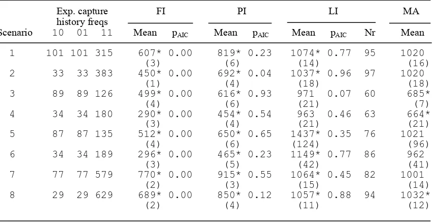
Simulation results appear in Table 1. Full independence and point independence

models had substantial negative bias in all scenarios, with full independence models

consistently more biased than point independence models. Within a scenario, the bias

was remarkably consistent, reflected in the very small standard errors of Table 1, but the

bias varied substantially between scenarios. Although the data were simulated from

limiting independence models, significant upward bias was found in six of the eight

scenarios when the data were analysed using the true model. However, the size of the

bias in most cases was substantially smaller than for point independence models.

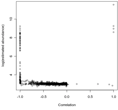
analyses under the limiting independence model were rejected due to high correlation

between αˆ and . Figure 1 shows the need to reject such cases; all of the very high

abundance estimates obtained correspond to a correlation between

j

0 ˆ

λ

αˆ and very close

to . In all cases use of AIC correctly diagnosed the presence of unmodelled

heterogeneity, although in some cases it did not differentiate well between point

independence and limiting independence scenarios.

j

0 ˆ

λ

1

±

4. Stake Data

Laake (1999) used data on a population of wooden stakes of known size to illustrate

independence issues in double-observer surveys. We use the same dataset here. The

surveys were conducted in 1977 and 1978 (Laake, 1978); as in Laake (1999), we

consider only the 1977 data. Multiple observers traversed a 1 km line marked with poles

at 100 m intervals and searched a strip of sagebrush-grassland habitat 20 m on either side

of the line for 150 wooden stakes that protruded 30 cm above ground. The stakes had a

random uniform distribution throughout the 1000 m × 40 m strip. Eight observers

separately surveyed the stakes, remaining on the line. Distances from the line were

measured accurately by an assistant.

For each pair of observers, we show estimates of abundance in Table 2. Models

were fitted corresponding to full independence (α =β =0), point independence

(α =0,β unconstrained) and limiting independence with α ≥0,β ≥0. In each case,

three models were fitted: the first with observer as a factor and distance as a covariate,

the second with the addition of an interaction term between the two, and the third with

the squared distance as an additional covariate, together with interaction terms between

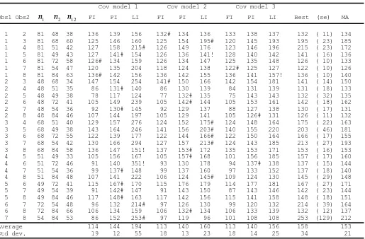
It is clear from Table 2 that models with all three forms of independence are

useful for the analysis of these data. Overall performance is remarkably good, with the

average of the best estimates (as judged by AIC) coming out close to the true abundance

of , as does the average of the model-averaged estimates, using AIC weights

(Buckland et al., 1997).

150

=

N

5. Shipboard Survey of Minke Whales

The second Small Cetacean Abundance in the North Sea and adjacent waters

(SCANS II) survey was a multinational survey conducted in 2005 by ship and aircraft to

estimate cetacean abundance in the North Sea, Kattegat, Skagerrak, western Baltic,

English Channel and the Celtic Sea. Double-observer line transect survey methods were

used because for many species detection of animals on the trackline was expected to be

less than unity. Details of the survey and further information can be found at

http://biology.st-andrews.ac.uk/scans2/. Here we analyse only shipboard survey data on

minke whales.

The methods used in the SCANS surveys were designed to break up the

dependence between the two observers, by ensuring that they are not simultaneously

searching the same patch of sea. A ‘tracker’ scans with high-powered binoculars well

ahead of the ship, and tracks detected animals in, to check whether the primary platform,

searching with hand-held binoculars and naked eye, detects them (so-called duplicate

detections). Previously, we have had no means of testing whether the method is

successful in breaking up the dependence between observers.

Using a truncation distance of 700 m, the tracker detected 54 minke groups

totalling 62 animals, while the primary platform detected 57 groups totalling 59 animals;

17 groups (19 animals) were detected by both tracker and primary platform.

) exp( 1 ) exp( ) , ( 2 1 0 2 1 0 z y z y z y p j j j j j j

j _{λ λ λ}

λ λ λ + + + + +

= , (6)

)} , ( ) , ( ){ , ( ) , ( ) ,

(y z =L y z +δ₀ y z U y z −L y z

δ (7)

where ⎭ ⎬ ⎫ ⎩ ⎨ ⎧ + − = ) , ( ) , ( 1 ) , ( ) , ( , 0 max ) , ( 2 1 2 1 z y p z y p z y p z y p z y

L , U(y,z)=min

{

}

and ) exp( )} , ( 1 { } 1 ) , ( { ) exp( )} , ( 1 { ) , ( 0 y z y L z y U y z y L z y β α β α δ + − + − + −

= . Covariate z is sea state

(Beaufort).

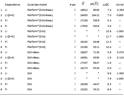
The benefits of field methods to break up heterogeneity are immediately apparent

from Table 3. AIC favours models with full independence (α =β =0), and selects the

model with identical detection functions for the two observers, and sea state as a

covariate. Estimation is largely unaffected by whether we assume full independence or

point independence. If we also relax the assumption of point independence, AIC values

are larger, but estimation is not greatly affected, with the exception of model 2.

Estimation is very similar to that reported by Burt et al. (unpublished). In that

analysis, no covariates were included, and point independence was assumed. Abundance

was estimated as with . The most comparable of our analyses

is model 7 of Table 3, for which and . AIC favours model 12,

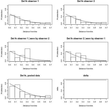
and corresponding fits are shown in Figure 2.

13281

ˆ ₌

N se(Nˆ)=4780

16192

ˆ ₌

N se(Nˆ)=4446

It is surprising that AIC favours models which assume the same detection

function for the two observers, given that the tracker is searching much further ahead of

the ship than the primary platform. However, estimation is barely affected by whether

we make this assumption or not. The distribution of distances from the line of detections

(Figure 2), although beyond this distance, the tracker detects more animals than the

primary platform.

6. Discussion

Our methods allow assessment of whether the full independence or point independence

assumptions are reasonable. The methods also provide a means of analysing

double-observer surveys without having to assume independence between the double-observers’

detection probabilities, even at distance zero. However, strong dependence between the

observers’ detection probabilities can lead to unreliable estimation. If possible, field

methods should be developed to ensure that there are not animals in the population that

are very unlikely to be detected, even if they are on the line. However, this strategy can

create problems for identifying duplicate detections, so that in some circumstances, it

may be preferable to estimate the proportion of animals that are essentially undetectable.

For example in aerial surveys of marine mammals, the observers might record only those

animals that are at the surface as they pass abeam, and a separate study might be used to

estimate the proportion of animals at the surface at any time.

Extension of the methods to point transect sampling is straightforward. We now

have if points are positioned randomly. In (4), the covered area a is now

, where K is the number of points. For , we obtain a similar result to

(5) by adapting equation (3.48) from Marques and Buckland (2004). 2

/ 2 )

(y = y w π

2

w K

a= π vaˆr(Nˆ)

It is knowledge of π(y) that allows us to weaken the full independence

assumption. In principle, the same approach could be applied to conventional

mark-recapture models, if π(y) were known for some explanatory variable y, although this

If there is responsive movement prior to detection so that the distances y available

for detection differ in an unknown way from that prior to movement (i.e. from π(y)),

then (a) δ(y) cannot be interpreted as above and (b) under the assumption of full

independence, δ(y) can be interpreted as a measure of deviation from π(y) due to

responsive movement. This can be seen from the following. The pdf of observed

distance for observer j is f_j(y₎₌ p_jj(y_{) (}y₎− ₍y_)/

∫

' | 1

'

| δ π δ π . If we

assume full independence, then is equal to the unconditional detection function

for observer j, and hence is proportional to the pdf of y after movement.

Note that while the interpretation of ) ( ' | y

p_jj

1 ) ( ) (_{y δ y} −

π

) (y

δ is different in this case from the case with no

responsive movement, the abundance estimator is still valid.

It is worth noting that although δ(y) is superficially similar to α(z) of Chen

(1999) and α of Chen and Lloyd (2000), it is in fact quite different. To see this, consider

a situation in which distance y and other variables u affect detection probability but only

y is recorded (in this case α(z) is a constant). Whereas α(z) and α quantify the

heterogeneity due to y, δ(y) quantifies the heterogeneity at y due to the unrecorded

variables u. This is an important difference because the formulations of Chen (1999)

and Chen and Lloyd (2000) do not accommodate heterogeneity due to the unrecorded

variables u, and it is precisely this heterogeneity that is at issue here. Chen (1999) and

Chen and Lloyd (2000) assume that p_•(y)= p₁(y)+ p₂(y)− p₁(y)p₂(y) whereas we

assume that p_•(y)= p₁(y)+ p₂(y)−δ(y)p₁(y)p₂(y). It is the discrepancy between the

shapes of and (j=1,2) which provides the basis for modelling

heterogeneity due to the unrecorded variables (together with knowledge of )

(y

f_j p_j|j'(y)

) (y

π ); the

) ( ' | y

p_jj and are therefore unable to exploit the information in the discrepancy between

the two. This applies equally to the case in which additional variables z are recorded

(but u remains unrecorded).

We have used AIC to select between models. We have estimated detection

functions by maximum likelihood, but abundance is estimated using a Horvitz-Thompson

estimator in which the inclusion probabilities have been estimated (by maximum

likelihood). As the components of the abundance estimators that are not estimated by

maximum likelihood (corresponding to sample size, and to extrapolation from the

covered area to the entire survey area) are common across models, it seems not

unreasonable to use AIC to select between abundance estimators. However, when some

inclusion probabilities are very small, modest error in estimating them can generate large

positive bias in the abundance estimate, which would be undetectable by AIC.

ACKNOWLEDGEMENTS

We thank Evan Cooch for generously providing computer time on his Linux machine.

We also thank the editors and referees of this and an earlier draft, which led to a

REFERENCES

Alpizar-Jara, R. and Pollock, K.H. (1996). A combination line transect and capture

recapture sampling model for multiple observers in aerial surveys. Environmental

and Ecological Statistics3, 311-327.

Borchers, D.L. (1996). Line Transect Estimation with Uncertain Detection on the

Trackline. PhD thesis, University of Cape Town.

Borchers, D.L. (1999). Composite mark-recapture line transect surveys. Pp. 115-126 in

Marine Mammal Survey and Assessment Methods, eds G.W. Garner, S.C.

Amstrup, J.L. Laake, B.F.J. Manly, L.L. McDonald and D.G. Robertson.

Balkema, Rotterdam.

Borchers, D.L., Buckland, S.T., Goedhart, P.W., Clarke, E.D. and Hedley, S.L. (1998a).

Horvitz-Thompson estimators for double-platform line transect surveys.

Biometrics54, 1221-1237.

Borchers, D.L., Buckland, S.T. and Zucchini, W. (2002). Estimating Animal Abundance:

Closed Populations. Springer-Verlag, London.

Borchers, D.L., Laake, J.L., Southwell, C. and Paxton, C.G.M. (2006). Accommodating

unmodeled heterogeneity in double-observer distance sampling surveys.

Biometrics62, 372-378.

Borchers, D.L., Zucchini, W. and Fewster, R.M. (1998b). Mark-recapture models for

line transect surveys. Biometrics54, 1207-1220.

Buckland, S.T., Anderson, D.R., Burnham, K.P., Laake, J.L., Borchers, D.L. and

Thomas, L. (2001). Introduction to Distance Sampling: Estimating Abundance

of Biological Populations. Oxford University Press, Oxford.

Buckland, S.T., Burnham, K.P. and Augustin, N.H. (1997). Model selection: an integral

Buckland, S.T. and Turnock, B.J. (1992). A robust line transect method. Biometrics48,

901-909.

Burt, M.L., Borchers, D.L. and Samarra, F. (unpublished). Abundance estimates from

SCANS-II: stratified analysis.

Chen, S.X. (1999). Estimation in independent observer line transect surveys for cluster

populations. Biometrics55, 754-759.

Chen, S.X. (2000). Animal abundance estimation in independent observer line transect

surveys. Environmental and Ecological Statistics7, 285-299.

Chen, S.X. and Lloyd, C.J. (2000). A nonparametric approach to the analysis of

two-stage mark-recapture experiments. Biometrika87, 633-649.

Innes, S., Heide-Jørgensen, M.P., Laake, J.L., Laidre, K.L., Cleator, H., Richard, P. and

Stewart, R.E.A. (2002). Surveys of belugas and narwhals in the Canadian high

Arctic in 1996. Scientific Publications of the North Atlantic Marine Mammal

Commission4, 169-190.

Laake, J.L. (1978). Line Transect Estimators Robust to Animal Movement. MS thesis,

Utah State University.

Laake, J.L. (1999). Distance sampling with independent observers: reducing bias from

heterogeneity by weakening the conditional independence assumption. Pp.

137-48 in Marine Mammal Survey and Assessment Methods, eds G.W. Garner, S.C.

Amstrup, J.L. Laake, B.F.J. Manly, L.L. McDonald and D.G. Robertson.

Balkema, Rotterdam.

Laake, J.L. and Borchers, D.L. (2004). Methods for incomplete detection at distance

zero. Pp. 108-189 in Advanced Distance Sampling, eds S.T. Buckland, D.R.

Anderson, K.P. Burnham, J.L. Laake, D.L. Borchers and L. Thomas. Oxford

Manly, B.F.J., McDonald, L.L. and Garner, G.W. (1996). Maximum likelihood

estimation for the double-count method with independent observers. Journal of

Agricultural, Biological, and Environmental Statistics1, 170-189.

Marques, F.F.C. and Buckland, S.T. (2003). Incorporating covariates into standard line

transect analyses. Biometrics59, 924-935.

Marques, F.F.C. and Buckland, S.T. (2004). Covariate models for the detection function.

Pp. 31-47 in Advanced Distance Sampling, eds S.T. Buckland, D.R. Anderson,

K.P. Burnham, J.L. Laake, D.L. Borchers and L. Thomas. Oxford University

Press, Oxford.

Palka, D. (1995). Abundance estimate of the Gulf of Maine harbor porpoise. Pp. 27-50

in Biology of the Phocoenids, eds A. Bjørge and G.P. Donovan. International

Whaling Commission, Cambridge.

Quang, P.X. and Becker, E.F. (1997). Combining line transect and double count

sampling techniques for aerial surveys. Journal of Agricultural, Biological, and

Environmental Statistics1, 170-189.

Schweder, T., Skaug, H.J., Langaas, M. and Dimakos, X.K. (1999). Simulated likelihood

methods for complex double-platform line transect surveys. Biometrics 55,

678-687.

Skaug, H.J. and Schweder, T. (1999). Hazard models for line transect surveys with

Table 1.

Mean (standard error in parentheses) of 100 abundance estimates under full independence (FI), point independence (PI) and limiting independence (LI) models for the eight simulation scenarios. The expected capture history frequencies are shown for each scenario. Also shown is pAIC, the proportion of times each model was selected by AIC, and model-averaged (MA) estimates, obtained by taking a weighted average of estimates from the above three models, using AIC weights. Where an LI model was deemed to be parameter-redundant (correl(αˆ,λˆ₀₁) >0.99), the model was not considered even if it had the best AIC value, and the weighted average was over the FI and PI models only. The mean and standard error for LI models is across only those runs for which the model was not deemed to be parameter-redundant. The number of runs (Nr) out of 100 contributing to the LI results under each scenario is shown. True abundance is 1000. *Bias significant at 5% level.

Exp. capture FI PI LI MA history freqs

Scenario 10 01 11 Mean pAIC Mean pAIC Mean pAIC Nr Mean

Table 2.

Estimates of abundance for the stake data for all combinations of the 8 observers under full independence, FI (α =β =0), point independence, PI (α =0,β unconstrained) and limiting independence, LI with

0 ,

0 ≥

≥ β

α . Covariate model 1 has covariate structure observer + distance, model 2 has structure

observer * distance, and model 3 has structure observer * (distance + distance2). ‘Best’ corresponds to the model with the smallest AIC (indicated by ‘#’, with standard error in parentheses), and ‘MA’ is the model-averaged estimate, using AIC weights. True abundance is 150. LI fits with

9 . 0 ) ˆ , ˆ (

correlα λ₀₁ > were not used for the best or model-averaged estimates, and are indicated by ‘!’.

Cov model 1 Cov model 2 Cov model 3

Obs1 Obs2 n₁ n₂ n₁₂ FI PI LI FI PI LI FI PI LI Best (se) MA

1 2 81 48 38 136 139 156 132# 134 136 133 138 137 132 ( 11) 134 1 3 81 68 60 125 146 160 125 154 195# 120 145 193 195 ( 23) 185 1 4 81 51 42 127 158 215# 126 149 176 123 146 196 215 ( 23) 172 1 5 81 49 43 127 141# 154 126 136 141! 128 140 142 141 ( 16) 136 1 6 81 72 58 126# 134 159 126 134 147 125 135 148 126 ( 10) 133 1 7 81 54 47 120 135 204 118 124 138 122# 125 127 122 ( 10) 126 1 8 81 84 63 136# 142 156 136 142 155 136 141 157! 136 ( 10) 140 2 3 48 68 34 147 154 254 141# 150 166 142 154 181 141 ( 14) 150 2 4 48 51 35 86 131# 140 86 130 139 84 131 139 131 ( 18) 133 2 5 48 49 38 78 117 124 77 132# 135 75 143 143 132 ( 32) 135 2 6 48 72 41 105 149 239 105 142# 144 105 153 161 142 ( 18) 162 2 7 48 54 36 92 130# 145 92 129 137 88 127 138 130 ( 17) 131 2 8 48 84 46 107 144 197 105 129 141 105 126# 131 126 ( 11) 132 3 4 68 51 40 129 157 276 124 152 175# 124 148 164 175 ( 22) 163 3 5 68 49 38 143 164 246 141 156 203# 140 155 220 203 ( 46) 181 3 6 68 72 55 122 139 177 122 144 166# 122 150 164 166 ( 17) 155 3 7 68 54 42 130 166 294 127 157 213# 124 143 185 213 ( 27) 193 3 8 68 84 58 136 147 151! 137 153# 172 135 153 171 153 ( 16) 153 4 5 51 49 33 105 156 167 105 157# 168 101 156 185 157 ( 17) 160 4 6 51 72 46 91 140 351! 93 130 178 94 137# 138 137 ( 15) 144 4 7 51 54 36 99 137# 148 99 137 160 97 133 152 137 ( 18) 140 4 8 51 84 48 107 141 222 106 124 145# 109 124 130 145 ( 29) 148 5 6 49 72 41 115 167# 170 115 176 179 114 177 181 167 ( 27) 171 5 7 49 54 39 91 142# 147 91 143 150 87 143 146 142 ( 23) 144 5 8 49 84 46 117 148# 163 117 142 156 115 141 158 148 ( 18) 151 6 7 72 54 48 96 132 214# 97 126 130 99 120 132 214 ( 39) 164 6 8 72 84 66 106 134 159 106 132# 134 106 133 139 132 ( 12) 137 7 8 54 84 53 86 152 253# 97 119 96 101 108 108 253 (129) 212

Table 3. Models fitted to the minke whale survey data. The full model, denoted here by LI (Limiting Independence), Platform*(Dist+Beau), is defined by equations (6) and (7). The estimates and were obtained by appropriate extensions of equations (3) and (4) for a stratified design. Correl for LI models with a platform effect corresponds to whichever of

Nˆ se(Nˆ)

) ˆ , ˆ (

correlα λ₀₁ and correl(αˆ,λˆ₀₂) is closest to 1. PI indicates Point Independence (α =0) and FI denotes Full Independence (α =β =0).

#  Dependence  Covariate model   # par   

Nˆ se(Nˆ)    ∆

  AIC  Correl

1  LI  Platform*(Dist+Beau)  8 16912  6663  7.4    0.393

2  LI (β=0)  Platform*(Dist+Beau)  7 26453  18422  7.0  ‐0.805

3  PI  Platform*(Dist+Beau)  7 17156  5359  5.4  ─

4  FI  Platform*(Dist+Beau)  6 17935  5436  3.6  ─

5  LI  Platform*(Dist)  6 *  *  13.6  ‐1.000

6  LI (β=0)  Platform*(Dist)  5 *  *  11.7  ‐1.000

7  PI  Platform*(Dist)  5 16192  4446  12.3  ─

8  FI  Platform*(Dist)  4 15195  3311  10.4  ─

9  LI  Dist+Beau  5 16837  7130  3.9    0.073

10  LI (β=0)  Dist+Beau  4 16091  4365  1.9    0.124

11  PI  Dist+Beau  4 17337  5647  1.9  ─

12  FI  Dist+Beau  3 18173  5534  0.0  ─

13  LI  Dist  4 *  *  9.8    1.000

14  LI (β=0)  Dist  3 *  *  7.9  ‐1.000

15  PI  Dist  3 16209  4447  8.5  ─

16  FI  Dist  2 15202  3313  6.6  ─

*correl(αˆ,λˆ_0j) >0.99 for j=1 and 2 (models 1-8) or correl(αˆ,λˆ₀) >0.99 (models

Figure 1. Plot of against , illustrating that the very high estimates

of abundance from the simulations all arose when was very close to . )

ˆ

log(N correl(αˆ,λˆ₀₁)

) ˆ , ˆ (

correlα λ₀₁ ±1

-1.0 -0.5 0.0 0.5 1.0

468

1

0

Correlation

lo

g(

est

im

a

te

d abundance)

Figure 2. Estimated detection functions for minke whales, model 12 (see Table 3). The

top left plot is the estimated unconditional detection function for observer 1, and top right is the estimated unconditional detection function for observer 2. The corresponding conditional detection functions are shown in the centre. Under this model, all four of these detection functions are identical, but the data in each plot differ. The estimated detection function for the two observers combined is shown at the bottom left. The bars are: relative frequencies of detections made by observer 1 (top left), relative frequencies of detections made by observer 2 (top right), proportion of observer 2 detections made by observer 1 (middle left), proportion of observer 1 detections made by observer 2 (middle right), and relative frequencies of detections made by at least one observer.

0.0 0.1 0.2 0.3 0.4 0.5 0.6 0.7

0.

0

0.

4

0

.8

Det fn observer 1

Distance from line

P

r(

det

ec

tion

)

0.0 0.1 0.2 0.3 0.4 0.5 0.6 0.7

0.

0

0.

4

0

.8

Det fn observer 2

Distance from line

P

r(

det

ec

tion

)

0.0 0.1 0.2 0.3 0.4 0.5 0.6 0.7

0.

0

0

.4

0.

8

Det fn observer 1 | seen by observer 2

Distance from line

P

r(

det

ec

tion)

0.0 0.1 0.2 0.3 0.4 0.5 0.6 0.7

0.

0

0

.4

0.

8

Det fn observer 2 | seen by observer 1

Distance from line

P

r(

det

ec

tion)

0.0 0.1 0.2 0.3 0.4 0.5 0.6 0.7

0.0

0

.4

0

.8

Det fn, pooled data

Distance from line

P

r(

d

ete

c

tion

)

0.0 0.1 0.2 0.3 0.4 0.5 0.6 0.7

0.0

0

.4

0

.8

delta

Distance from line

de