Online Full Text



Abstract— A numerical method using a combination of a radial and a polynomial basis function called the radial point interpolation method (RPIM) is studied in this work. The spatial discretization is completed using the Matern radial type of basis function where the 4th-order Runge-Kutta is adopted for tackling the transient term. One of the most complicated structures of PDEs namely Burgers’ equations is numerically solved by the method aiming to evaluate the method’s effectiveness. To justify the advantage of the Matern RBF, a study based on the most popular choice of RBF called ‘Multiquadric MQ’ is also carried out parallelly. All solutions obtained from the RPIM application are validated against the exact solution and also with other numerical works when available in literatures. RPIM has shown promising results and with the use of Matern RBF, the conditioning problem is found to be greatly reduced with higher accuracy even with very high Reynolds number.

Index Terms— coupled-Burgers’ equations, numerical solution, Radial Point Interpolation Method (RPIM), Matern RBF.

I. INTRODUCTION

ITH a number of clear advantages over the traditional finite element method (FEM), a new class of numerical methods known as ‘meshless/meshfree’ have recently been receiving great amount of interest from scientists and engineers. By linking the randomly chosen computational nodes simply with a linear combination of a certain set of functions; with certain properties, mesh generating process is out of requirement as remained the case for FEM. Some different versions of this kind are the element-free Galerkin method [1], the local Petrov-Galerkin [2, 3], and meshless manifold method [4], please also see references therein. Amongst those under the same name of ‘meshless/meshfree’ methods, our attention is paid to those concerned with collocation process. Along this track, Kansa, nevertheless, is known to severely suffer from having a fully unsymmetric and populated collocation matrix, increasing the risk of being ill-conditioned. The problem becomes even more severe when the number of nodes is increasing or with larger domain.

Manuscript received June 10, 2018; revised July 19, 2018.

S. Kaennakham, School of Mathematics, Institute of Science, Suranaree University of Technology, Nakhon Ratchasima 30000, Thailand

Centre of Excellence in Mathematics, Bangkok 10400, Thailand (corresponding author: [email protected] )

N. Chuathong, Faculty of Science Environment and Energy, King Mongkut’s University of Technology North Bangkok (Rayong Campus), Rayong 21120, Thailand (e-mail: [email protected]).

One of the improved versions of the traditional Kansa collocation schemes designed to alleviate all those previously mentioned undesired features is the attempt to combine the radial basis function and some polynomial basis functions. This idea was proposed in 2002 by Wang and Liu [12] and it has been known as ‘The Radial Point Interpolation Method (RPIM)’. With this method, the approximation of the solution is obtained by letting the interpolation function pass through the function values at each scattered node within the domain. One of the nice numerical experiments on applying this methods is that carried out by Liu [13] in 2011, where it was concluded that by using the combination of radial and polynomial basis functions, the singularity problem can be improved. Together to this, the effect of shape parameters on the method for elastoplastic problems in two-dimension models using MQ-RBF was documented by Bozkurt et. al. [14] in 2013. For some more recently and nicely documented, the interested reader is referred to [15] and [16], please see also the references therein.

For all collocation-based meshless methods mentioned so far, it is the Radial Basis Function that plays a crucial role in determining the quality of the final results. Since the beginning of the idea of collocation, it has been the so-called Multiquadric RBF or ‘MQ’ that remains the most popular choice. While good solutions can be produced in some certain problems, MQ is known to carry some undesirable properties particularly the conditioning problem. Over the past decade, a great amount of attention has been paid to this kind of radial basis function where as there is one type that has not been explored as much. It is called ‘Matern Radial Basis Function (MTrn-RBF)’. In this work, the main task is to look at this kind of RBF hoping to shed more light into its numerical capability with applied with RPIM. The numerical test case chosen for this investigation is the transient, nonlinear and coupled-Burgers’ equations.

The famous ‘Burgers’ equations’, a system of equations that describes the interaction between two crucial physical manners of nature; convection and diffusion, is used to model variety of applications. This includes flows through a shock wave traveling in viscous fluid, the phenomena of turbulence, sedimentation of two kinds of particles in fluid suspensions under the effect of gravity and also dispersion of pollutants in rivers, see Burgers [17], Nee and Duan [18] , and Esipov [19]. Its one-dimension version has been widely studied including the application of two high-order numerical methods carried out by Pan [20], see also [21].

A Radial Point Interpolation Method (RPIM)

with Matern RBF Applied to a

Two-Dimensional Nonlinear Coupled-PDE

S. Kaennakham, and N. Chuathong

W

IAENG International Journal of Applied Mathematics, 48:4, IJAM_48_4_17

More recent numerical work, proposed in 2018, where the finite difference method in FT CS implicit scheme was applied to the modified form of Burgers’ equation and it can be found in Sungnul et.al. [22].

For two-dimension form, some of the recent computational ones include the application of a fully implicit finite-difference (see [23]), by Adomain-Pade technique (see [24]), by adopting variational iteration method (see [25]), by applying a meshfree technique (see [26] and [27]). Even more recently, more numerical works have been successfully carried out and nicely documented in literature; the application of the dual reciprocity boundary element method (see [28] and [29]), POD/discrete empirical interpolation method (DEIM)-reduced order model (ROM) (see [30]), and a combination between the homotopy analysis method and finite differences (see [31]).

The organization of this work is as follows. The fundamental of both the Radial Point Interpolation Method and the chosen Matern RBF is detailed in Section 2 where its implementation both spatial and time are provided in Section 3. Section 4 presents the overall performance of the method when applied to the test case. Some interesting results obtained are also discussed in the same section before Section 5 summarizes the main important findings achieved from the whole experiment.

II. MATHEMATICALBACKGROUND

A. Radial Point Interpolation Meshfree Method

Given a bounded and connected domain



with



being the domain boundary containing two non-overlap sections; ₁and₂, with  _{1 2} . Let

 

1 n c

j _j



X x be

a set of randomly selected points, known as ‘centers’. The radial point interpolation scheme writes the approximate solution for a given PDE,u x( ) as the linear combination of the basis function



 

:



n

j

  and monomialsp x_j

 

, shown in the following form;



2



 

1 1

T T

( ) ( )

.

n m

i i j j

i j

u u R a p b

 

  

 





x x x x x

R (x)a P (x)b

(1)

This is defined for a center

x

in a support domain

  _x that contains n surrounding nodes, or is the total number of centers in case of global collocation as adopted in this work, and m representing the number of polynomial basis (usually, mn). R



xx_{i 2}



is the so-called ‘Radial

Basis Function’ whose values depends only on the distances

between the centers, x, and their surrounding nodes

x

_i

measured with the Euclidean norm 2

. in 2D. The polynomial function can be chosen from Pascal’s triangle which, for 2D problems, is of the following form;

2 2

1, , ,x y x xy y, , ,...

 

  

T

P (x) (2) With this additional term, the interpolation is enforced to pass thought all those nodes in the support domain.

To ensure the unique solution of the system, additional equations shall be added as the constraint conditions, as

follows;

T

1

( ) 0

n

j i i m i

p a



 



x P a (3)

For j1, 2,...,m. This leads to the following form of matrix equations describing the interpolation process for all centers all over the domain.

0

0 ( )

( ) _T m

m       _{ }_{  }      R P

U x a

U x Hα

P 0

0 b (4)

Leading to

1

0 ( )





α H U x (5)

Where _T0 m

m        R P H

P 0 ,

  



0 , 1 2 ... , 1 2 ...

T T

n m

a a a b b b

 

α a b

1 1 1 2 1 1 1 1

1 2 2 2 2 2 2 2

0 1 2 ( , ) ( , ) ... ( , ) ( , ) ( , ) ... ( , ) ( , ) ( , ) ... ( , ) n n

n n n n n n n n n

R x y R x y R x y R x y R x y R x y

R x y R x y R x y _

             R 1 2 1 2 1 2

1 1 ... 1

... ...

(x ) (x ) ... (x )

n T

m n

m m m n m n

x x x

y y y

p p p _

                 P

Substituting these back into the collocation equation, yielding;

T T 1

( ) ( )

u x  R (x) P (x) H U x_  (6) By setting the shape functions matrix,_{Θ (x)}T _{, as;}

T  T T  1

  

Θ (x) R (x) P (x) H (7)

Then the previous equation can be re-written as; T

( ) ( )

u x Θ (x)U x (8) Where the approximate solutions at each center can now be obtained.

B. Radial Point Interpolation Meshfree Method

In order to alleviate the problem of conditioning usually encountered when utilizing a rather popular choice of RBF namely Multiquadric, another class of RBFs that have not been receiving as much interest is focused on in this work. This is known as ‘Matern Radial Basis Function’ and those categorized in this family are defined in general form as;

 

2

   

1

 

r r r

          

 (9)

When



 

2



2

2

i j i j i j

r x x  x x  y y and this can lead to another relation, in case is a positive integer.

   















 



1 0 2 exp !

2 1 ! ! ! 2

n _n

k

n _k

r r n k

r

n k n k r

     _   





 (10)

Where



_ is a modified Bessel function of order



, with being a parameter that is smooth and



is the parameter as generally found in most forms of RBFs? In this work, the values of



are particularly chosen and they are as follows;

 • If





1/ 2

, this gives the Basic Matern ;

IAENG International Journal of Applied Mathematics, 48:4, IJAM_48_4_17

 

r exp( )



 



x (11)

 If





3 / 2

, this gives the Linear Matern (referred to as ‘LMTrn’) :

 

r



1



exp( ),



 



x 



x (12)

 If





5 / 2

, this gives the Quadratic Matern

(referred to as ‘QMTrn’)

 







2



3 3 exp( ),

r

    x   x  x (13)

 If





7 / 2

, this gives the Cubic Matern (referred to as ‘CMTrn’)

 





 

2



3



15 15 6 exp( )

r

    x   x   x  x (14)

Nevertheless, the Basic Matern is not applicable in this work since it is not differentiable at the origin. Interestingly, this family of basis function has not been looked at as much when compared to other kinds. One positive aspect that Matern RBF has is pointed out by Stein [32] in 1990 where it was stated in their work that the ‘degree of smoothness to be estimated from the data rather than restricted a priori’. It can be interpreted as that if the data is determined to be smooth, a higher value of



would be appropriate and, similarly, if the data is noisy, then a lower value of



should be adopted. In this work, however, only 3 values of



are under the investigation; Equation (12)-(13)-(14).

III. MATHEMATICALBACKGROUND

With its rich in challenging Figs for being solved numerically, the well-known ‘Burgers equations’ are particularly chosen to be the test case of this study. The discretization in space and time are detailed in the following subsections.

A. The Transient Nonlinear Coupled-Burgers’ equations

Known as a simple case of the Navier-Stoke equation, the famous ‘Burgers’ equations’ , a system of equations that describes the interaction between two crucial physical manners of nature; convection and diffusion, is used to model variety of applications. This includes flows through a shock wave traveling in viscous fluid, the phenomena of turbulence, sedimentation of two kinds of particles in fluid suspensions under the effect of gravity and also dispersion of pollutants in rivers, see [20-22].

The standard form of this type of equation is expressed as;

2 2

2 2

1

u

u

u

u

u

u

v

t

x

y

Re

x

y









































(15)

And

2 2

2 2

1

v

v

v

v

v

u

v

t

x

y

Re

x

y









































(16)

The ratio of inertial forces to viscous forces is represented by the Reynolds number,

Re

characterizing the relative strength of inertial forces to viscous forces. The relative strength of these two actions - their ratio - does have a lot of influence on how the fluid flow behaves. The x- and y-velocity components are noted by u x y t



, ,



and v x y t



, ,



respectively.

For a domain  





x y,



:ax y, b



with its boundary



, the above system is subject to the following initial conditions;



, , 0



1

 

, , ,

 

u x y 



x y x y  (17)



, , 0



2

 

, , ,

 

v x y 



x y x y  (18) And the boundary conditions;



, ,



1



, , , ,



, 0,

u x y t 



x y t x y t (19)



, ,



2



, , , ,



, 0,

v x y t 



x y t x y t (20) Here   ₁, , _{2 1} and ₂ are known functions.

In 1983, Fletcher [33] applied the Hopf-Cole transformation and successfully solved the equation analytically. Ever since, the coupled two-dimensional Burgers’ Equations have been attracting a number of investigations both numerically and analytically.

B. Discretization in Space

With the Radial Point Interpolation technique, it begins with writing the approximation of solution for (15) and (16), respectively, with the same radial basis function R x

 

and a polynomialP x( ), as follows;

T T

1 2

( )

u x R (x)a P (x)a (21) And

T T

1 2

( )

vx R (x)b P (x)b (22) Note that

u x

( )

and

v x

( )

can well be formed using the same both radial basis function and the additional polynomials;

P (x)

T

 



1

x y x

2

xy y

2





,

i.e.m6 , is needed to be imposed in order to obtain the coefficient matrices

 

a and. The necessary conditions for this task are expressed as follows;

  

1 1

1

0,

n

T

j i _i m

i

p

a









x

P a

(23)

For

j



1, 2,...,

m

. And;

  

1 1

1

0,

n

T

j i i m

i

p

b









x

P b

(24)

For

j



1, 2,...,

m

. Making equation (21) and (22) come to the same matrix system as explained in Equation (4) which can be re-written in a general form as shown below ;

 

m 1

( )

T m 



 



 

 











R

P

U x

α

P

0

0

(25)

When implemented to the Burgers’ equations, with

n

being the number of centers, uniformly distributed in this work, over the domain, the method transforms the governing equations to the following matrix system;





 

1 1 Re x x dig t n y y dig   _{  }          _{  }    _{   }  _  

A C u R P

U a

v R P

(26)





1 1 Re x x dig t n y y dig   _{  }        _{    }     _{   }  _  

A C u R P

V b

v R P

(27)

IAENG International Journal of Applied Mathematics, 48:4, IJAM_48_4_17

For

i



1, 2,...,

n

and with the following matrices;

 



 









 









 







11 12 1

21 22 2

1 2

xx yy xx yy xx yy

n

xx yy xx yy xx yy

n

xx yy xx yy xx yy

n n nn n n

R R R R R R

R R R R R R

R R R R R R

         _{  }                A

 



 









 









 







11 12 1

21 22 2

1 2

xx yy xx yy xx yy

m

xx yy xx yy xx yy

m

xx yy xx yy xx yy

n n nm n m

P P P P P P

P P P P P P

P P P P P P

         _{  }                C 1 2 0 0 0

0 0 0

,

0 0 0

0 0 0 dig

n n n

u u u _           _{  }     u 1 2 0 0 0

0 0 0

0 0 0

0 0 0 dig

n n n

v v v _           _{  }     v

 

   

11 1 2 ...

       

1 2 1 2 2 2 3 ...

 

2

T

n m

a a a a a a a

 

  

a

And

   

11 1 2 ...

       

1 2 1 2 2 2 3 ...

 

2

T

n m

b b b b b b b

 

  

  b 

Other notations appeared are defined as;

2 2, B B   

 and

B B

  

 with RijR



, xixj 2



being the radial basis function, Matern type in this case, and with also a non-negative shape parameter



. With the same polynomial constrains, this leads to a transformation of equation (26) and (27) into a new system of equations where the solutions exist and are mathematically unique, and are expressed as follows;

 

 1 t

n m 

 

 

  

 

 T   

Ξ Ψ U

a

P 0 0 (28)

 1 t

n m 

 

 

    

   

 T   

Ξ Ψ V

b

P 0 0 (29)

Where

 

1

 

Re

x y

dig





dig



































Ξ

A

u

R

v

R

and

 

1

 

Re

x y

dig

 

dig

 

















 







 

Ψ

C

u

P

v

P

C. Discretization in Space

For the discretization in time, the 4th-order Runge Kutta,

RK-4, is adopted for this task and it begins with setting;





1 ˆ _Re x x dig y y dig  _{  }          _{   }  _  

A C u R P

Α

v R P

(30) And





1 ˆ Re x x dig y y dig  _{  }          _{   }  _  

A C u R P

Β

v R P

(31)

Hence, equation (28) and (29) respectively becomes;

 



 



1

ˆ _, k

t n d F t dt      

 U U Α a U (32)

 





1

ˆ _, k

t n d G t dt       _{ }

 V V Β b V (33)

Letting u



x,t k



u k , x 2 and v



x,t k



v k , x 2 , a time step size



t

, with also the following settings;

   





1 , ,

k k

tF t

   U

  1  

2 , ,

2 2

k k t

tF  t

   _   _

U 

  2  

3 , ,

2 2

k k t

tF  t

   _   _

U 

   





4 3,

k k

tF t t

   U   

The solution at the next time step,

t

k1is then;

 1  





1 2 3 4

1

2

2

6





 













k k

U

U

(34)

Similarly, the same manner can be carried out for

V

k1

D. Solution Algorithm

Each experiment carried out in this work is completed following the algorithm stated below;

Step 1 Choose

N

collocation or center

nodes

 

1 

 N

c j _j

X x , on the domain



Step 2 Specify the desired values of; 1)The Reynolds number (Re). 2) The final time

t

.

3) The time step



t

.

4) The Gaussian shape parameter



.

Step 3 Compute the initial collocation matrices

 

R x and P x( ) using the initial RPIM approximation, Equations (21)-(22).

Step 4 Apply the initial conditions;U 0 , V 0 , to get

 

a and  _{ }b from Equation (25).

Step 5 Compute the solutions for the next time step using the RK-4 time-discretization explained in Section 3.3.

Step 6 Construct the matrices Α and Β in the forms expressed in Equations (30)-(31) using the solutions previously obtained in Step.5.

Step 7 Use the solution from Step 5 to produce a new pair of

 

a , and _{ }b .

Step 8 Put what have been obtained from Step 6 and Step 7 into the RK-4 time-discretization, equation (32) – (33) to achieve solutions at the next time step.

Step 9 Carry on Step 6 - 8 until reaching the final time step

t

.

All computing experiments carried out in this study were executed on a computer notebook: Intel(R) Core(TM) i7-5500U CPU @ 2.40GHz with 8.00 GB of RAM and 64-bit Operating System.

E. Solution Validation Means

To justify the quality of the method in this study, solutions obtained are validated against both their exact formula and

IAENG International Journal of Applied Mathematics, 48:4, IJAM_48_4_17

those presented in literature, where available. Error measurement norms utilized are as follows;

1) Maximum Error (

L

_)

   

1

max

  _{ } i  i

i N

L u x u x (35)

2) Root-Mean-Square Error (L_rms)



   



1/ 2 2

1

1



 

   







N

rms j j

j

L u u

N x x (36)

3) Average-Error (Average-Error)

In addition to these norms, the results presented below are sometimes referred to as ‘and it is to be understood as;

 

 

2

 





  L U L V

Average L (37)

Where L U

 

and L

 

V are, respectively, that of that of

U



and

V



velocity component.

IV. MATHEMATICALBACKGROUND

A. Example 1

The example being numerically carried out is the well-known form of Burgers’ equations where its exact solutions for validation are provided by using a Hopf-Cole transformation nicely documented by Fletcher [33] in 1983 and expressed as follows;





1

3 1 Re

( , , ) 1 exp( 4 4 )

4 4 32



 

  _     _

 

u x y t x y t (38)





1

3 1 Re

( , , ) 1 exp( 4 4 )

4 4 32



 

  _     _

 

v x y t x y t (39)

Where both the initial and boundary conditions to be imposed to the equation system are generated directly from the above exact form over the domain



( , ) :0 1, 0 1



  x y  x  y as shown in Fig 1. With its rich of challenging features, the equations have been receiving interests from a number of researchers and been treated with variety of different numerical techniques.

Solutions obtained from applying the Radial Point Interpolation method are validated by comparing to both those documented in literatures and those provided by the exact formula, Equation (38) – (39).

Firstly, the issue of risking the ill-conditioned stage caused by the popular choice of RBF called ‘MQ’ is addressed. This can be monitored by the so-called ‘Condition Number’ expressed as;

1

2 2

( ) 

Cond Z Z Z (40) Where Zis the collocation matrix. i.e. Αˆ in Equation (30), and Bˆ in Equation (31) in this work. The outcome of this very first experiment is illustrated in Fig 2. The chosen Reynolds number of Re = 500is meant to represent the whole range of Reynolds number under this work. It has been found that by using Matern RBF, the sensitivity to perturbations of a linear system attributed to the collocation matrix can be noticeably reduced when compared to the conventional MQ-RBF. This gives some confidence for the next phase of study. This example is split into two main parts; one concerned with low- to moderate- Reynolds

number cases,



1Re500



, and the other with relatively high value of Reynolds number,



500Re 1, 200



. As previously mentioned, the so-called Reynolds number plays crucial rules in representing the ratio of forces exerted in the system and this is known to remain as one of the most challenging tasks to simulate both numerically and experimentally. Note also that the number of center nodes represented by

n

in Section 2 is to be referred to as nN from now on.

1) Case-I: Low - Moderate Reynolds Number

In order to validate the effectiveness of the method studied in this work, for this particular case of PDEs, it is crucial to ensure that the method works comparatively well with the cases with low Reynolds number. Low Reynolds number indicates the ratio of inertial forces to viscous forces which is considered the first challenge for any numerical methods proposed in literature.

Particularly, for this example, it is well-known that with the Reynolds number ranking in the interval1 Re 500can be considered as Low – Moderate Reynolds number.

Fig. 1. (a) A computational domain

Ω

with

20 20



uniformly-distributed center nodes, and (b) Exact

U



velocity profile at

Re 1.0



at

t



0.1

.

IAENG International Journal of Applied Mathematics, 48:4, IJAM_48_4_17

[image:5.595.321.527.323.717.2]

The first case is at

Re = 100

, the experiment was carried out usingt0.0001,



1.0,t2.0, and the number of center nodes is N21 21 with the main results being shown in Table 1 and Table 2. At this low Reynolds number, it can be seen from the Tables that solutions produced numerically by all three Matern RBFs are in reasonably good agreement with both the corresponding exacts and those done and presented by other authors in literature.

Nevertheless, it has to be noticed that while the results are found to at the similar level of accuracy, only

441

nodes were required while other works employed much more nodes to be involved. The choice of shape parameter of was chosen based on a pure guess before another set of experiments were proceeded aiming to measure the effect of the shape parameter on the overall accuracy and the results obtained are displayed in Fig 3.

From Fig 3, the results show that the parameter of the CMTrn becomes less sensitive to the error norm meaning that the computing process is more likely to provide stable solutions when using



0.3. This gives some confidence for the experiments previously done and results have already been discussed. Since, from now on, the effectiveness of the method proposed in this work will be validated against

one of the most popular choice of RBF namely ‘Multiquadric-RBF (MQ)’, Fig 4. also provides some information on the effect of shape parameter and in general, it is found that with



1.0 the solution should be reliable and not to be severely affected by . The simulations carried out for comparison purposes hereafter, therefore, shall be based on this information.

Based on information provided from pervious experiments, a large series of numerical test cases were carried out in order to cover the whole range of Reynolds number , i.e.1 Re 500, with the main results being documented in Table 3 and Table 4. With



1.5, t 0.001,t1.0, and the number of nodes is

10 10

N  there are some interesting figures revealed. Except for the case at moderate Reynolds number, i.e.

Re



500

, solutions generated numerically by all Matern forms and MQ are in reasonably good with the exact solutions indicating by1.00E05Lrms 1.00E02. As

soon as Re reaches 400 and above, on the other hand, the solution obtained from MQ suddenly loses its accuracy by one order of magnitude. When consider only those three forms of Matern, the Linear one is clearly found to be comparatively worst in producing accurate results. Both Quadratic and Cubic forms are interestingly seen to arrive at the same level of accuracy for all cases of Reynolds number under investigation.

In overall results obtained, nevertheless, it is promising that RPIM applied with Matern class of RBF is capable of providing reliable results for the cases of low to moderate Reynolds number, Fig 5. This overall outcome finding from the experiments led to further investigations on cases with higher Reynolds number where it is known to be much more numerically challenging.

TABLE I

U

-VELOCITY AT FOR

Re 100



,



1.0, AND t2.0AND

21 21.

N 

(x,y) (0.1, 0.1) (0.3, 0.3) (0.5, 0.5) (0.1, 0.9) (0.5, 0.9)

Exact 0.500482 0.500482 0.500482 0.744256 0.555675 LMTrn 0.500125 0.501112 0.500305 0.744256 0.554951 QMTrn 0.501052 0.500122 0.500142 0.744158 0.556015 CMTrn 0.501022 0.510251 0.500152 0.74415 0.552143 [34] 0.50047 0.500441 0.500414 0.744197 0.554489 [27] 0.50035 0.50042 0.50046 0.74409 0.55604 [35] 0.50012 0.50042 0.50041 0.74416 0.55637 [23] 0.49983 0.49977 0.49973 0.7434 0.55413

TABLE II

V

-VELOCITY AT

Re 100



WITHt0.0001,



1.0,

2.0

t , AND N21 21

(x,y) (0.1, 0.1) (0.3, 0.3) (0.5, 0.5) (0.1, 0.9) (0.5, 0.9) Exact 0.999518 0.999518 0.999518 0.755744 0.944325 LMTrn 0.999458 0.994712 0.998701 0.754715 0.943955 QMTrn 0.999102 0.998251 0.997895 0.755821 0.944514 CMTrn 0.99775 0.98971 0.99901 0.75504 0.94602

[34] 0.99953 0.999559 0.999586 0.755803 0.945511 [26] 0.99936 0.99951 0.99958 0.75592 0.94392 [35] 0.99946 0.99938 0.99941 0.75558 0.94345 [23] 0.99826 0.99861 0.99821 0.755 0.94345

TABLE III

rms

L -ERROR FOR

U

-VELOCITY WITH



1.5, t 0.001,

1.0

t , AND N 10 10

Re LMTrn QMTrn CMTrn MQ

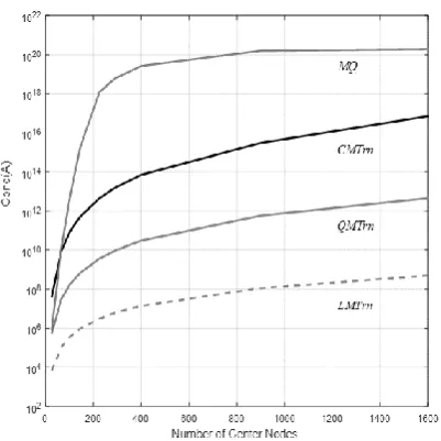
[image:6.595.65.266.344.545.2]

1 4.56E-02 4.31E-05 4.31E-05 1.41E-05 50 5.07E-03 8.82E-03 8.68E-03 8.69E-03 80 1.39E-02 1.60E-02 1.56E-02 1.63E-02 200 3.93E-02 3.78E-02 3.73E-02 9.25E-02 500 6.36E-02 6.54E-02 6.85E-02 3.93E-01 Fig. 2. Condition number when increasing the number of center

nodes at

Re



500

witht0.001,1.2, andt0.5.

IAENG International Journal of Applied Mathematics, 48:4, IJAM_48_4_17

2) Case-II: Moderate - High Reynolds Number

With the increase of the Reynolds number, it means that the viscous force of the system become more dominated by the inertial once. The phenomena is a transition of the flow from laminar to the state with much more complicated details known as ‘Turbulence’. The flow is typically turbulent with lots of large and small scale swirling motions (called eddies or vortices) and the flow can be quite chaotic on small scale even when the gross flow is fairly steady and smooth on average. This is known to remain one of the most challenging tasks for any numerical scheme aiming to mimic

this kind of natural transition phase. In the past decade, in particular, there has been a great deal of numerical works under the investigation of finding the solutions to this transition and some are listed in Table 5.

In this study, for the case of higher Reynolds number, it begins with investigating the general effect of the increase of Reynolds number where the solution errors produced by the RPIM are measured by the chosen error norms. Table 6 and Table 7 respectively provides both L_ and L_rms error norms for

U

-velocity and

V

-velocity computed using

2.5



 ,  t 0.01, t1.0, and N30 30. As can be anticipated, the numerical method loses its accuracy when the Reynolds number increases and yet, those obtained from using Matern family of RBF are still seen to maintain the level of accuracy around 1.50E01, even when

Re

reaches

1,200

.

TABLE IV

rms

L -ERROR FOR

V

-VELOCITY WITH



1.5 ,  t 0.001,

1.0

t , AND N 10 10

Re LMTrn QMTrn CMTrn MQ

[image:7.595.321.539.289.554.2]

1 6.42E-02 6.22E-05 6.22E-05 1.83E-05 50 1.78E-02 8.71E-03 8.67E-03 8.73E-03 80 2.16E-02 1.59E-02 1.56E-02 1.64E-02 200 4.15E-02 3.77E-02 3.73E-02 9.26E-02 500 6.41E-02 6.53E-02 6.85E-02 3.93E-01

Fig. 3. The effect of Cubic Matern shape parameter at

Re 100



with t0.001, andt0.5. [image:7.595.63.272.603.759.2]

Fig. 4. The effect of Multiquadric shape parameter at

Re



400

with t0.001, andt0.5.

Fig. 5.

U

-velocity profile from at

Re



50

withN20 20 ,

0.001,

t

[image:7.595.323.541.617.755.2]

 1.0and t0.5; (a) QMTrn, and (b) the exact solution.

Fig. 6. The effect of the number of centers at

Re



700

with  1.5, t0.001, and

t



2.0

.

IAENG International Journal of Applied Mathematics, 48:4, IJAM_48_4_17

With comparison taken only amongst those three Matern RBFs, the increase of Reynolds number is seen not to have significant effect on the solution quality. The Cubic form of Matern, nevertheless, is noticed to remain in comparatively best agreement with the exact solutions, and yet are also very close to those obtained by Quadratic Matern RBF.

The Linear form of Matern produces results with highest error magnitude with the maximum values of,

3.205 01

AverageL_ E and AverageLrms7.37E02

are found at the case of Re = 1,200 as expected.

This data presented in Table 6 and Table 7 is once more confirmed by the study of the center nodes density as illustrated in Fig 6 and Fig 7. In these two Figs, a large number of simulations were performed using

Re



700

with



1.5,t0.001 and the results were recorded at

2.0

t . The number of center nodes was set to cover a wide range starting from the smallest N 5 5 up to the highest

aboveN40 40 . The results calculated by MQ-RBF are clearly seen to be severely influenced by the increase of nodes density over the computational domain, with the going beyond AverageL_rms1.0E20 whenN600. On the other hand, those produced by Matern-RBF are insignificantly affected by the increase ofN, particularly when Nabove600. Within Matern family, the linear form is once again seen to have the highest value of error magnitude where the other two are comparatively in best agreement with the exact solutions and also stay close to each other with largeN.

Based on the results being under discussion so far, nevertheless, it has to be noticed that the choice of shape parameter,



, used for both MQ and Matern RBF can well be arguable. This is because it is known in many investigations (see [29, 41]) that MQ type of RBF can also be sensitive to its shape parameter. The assumption made based on Fig 4; run at

Re



400

with

0.001,

t

 and

t



0.5

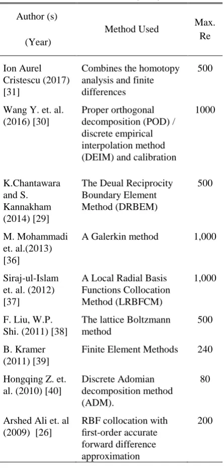
, may not be valid or reliable for cases with much higher Reynolds numbers as the interaction between those two forces has dramatically changed.

TABLE V

NUMERICAL WORKS DONE WITHIN THE PAST DECADE WITH THE REYNOLDS NUMBER,

Re

, INVOLVED

Author (s) (Year)

Method Used Max.

Re

Ion Aurel Cristescu (2017) [31]

Combines the homotopy analysis and finite differences

500

Wang Y. et. al. (2016) [30]

Proper orthogonal decomposition (POD) / discrete empirical interpolation method (DEIM) and calibration

1000

K.Chantawara and S. Kannakham (2014) [29]

The Deual Reciprocity Boundary Element Method (DRBEM)

500

M. Mohammadi et. al.(2013) [36]

A Galerkin method 1,000

Siraj-ul-Islam et. al. (2012) [37]

A Local Radial Basis Functions Collocation Method (LRBFCM)

1,000

F. Liu, W.P. Shi. (2011) [38]

The lattice Boltzmann method

500

B. Kramer (2011) [39]

Finite Element Methods 240

Hongqing Z. et. al. (2010) [40]

Discrete Adomian decomposition method (ADM).

80

Arshed Ali et. al (2009) [26]

RBF collocation with first-order accurate forward difference approximation

200

TABLE VI

ERROR MEASUREMENT FOR U-VELOCITY WITH



2.5, t 0.01,t1.0, AND N30 30

Re

L



LMTrn QMTrn CMTrn MQ

600 2.98E-01 2.67E-01 2.58E-01 3.09E+27 800 3.11E-01 2.78E-01 2.69E-01 6.39E+56 1000 3.17E-01 2.83E-01 2.73E-01 1.70E+59 1200 3.20E-01 2.86E-01 2.76E-01 6.86E+63

Re

L

rms

LMTrn QMTrn CMTrn MQ

[image:8.595.57.280.102.567.2]

600 6.56E-02 6.25E-02 6.20E-02 4.99E+26 800 6.93E-02 6.63E-02 6.49E-02 1.60E+56 1000 7.18E-02 6.87E-02 6.61E-02 3.79E+58 1200 7.36E-02 7.03E-02 6.68E-02 1.75E+63

TABLE VII

ERROR MEASUREMENT FOR U-VELOCITY WITH



2.5, t 0.01,t1.0, AND N30 30

Re

L



LMTrn QMTrn CMTrn MQ

600 3.00E-01 2.67E-01 2.58E-01 3.09E+27 800 3.12E-01 2.78E-01 2.69E-01 6.39E+56 1000 3.18E-01 2.83E-01 2.73E-01 1.70E+59 1200 3.21E-01 2.86E-01 2.76E-01 6.86E+63

Re

L

rms

LMTrn QMTrn CMTrn MQ

600 6.60E-02 6.25E-02 6.20E-02 4.99E+26 800 6.97E-02 6.63E-02 6.49E-02 1.60E+56 1000 7.20E-02 6.87E-02 6.61E-02 3.79E+58 1200 7.38E-02 7.03E-02 6.68E-02 1.75E+63

IAENG International Journal of Applied Mathematics, 48:4, IJAM_48_4_17

In order to provide answer to this skeptical aspect, a series of numerical test were carried out aiming to pinpoint the ‘Optimal opl’ value of MQ-shape parameter at a certain set of conditions;

Re



900

with  t 0.001, and

t



0.5

.

The results obtained from this small experiment, not shown here, indicates that the lowest Average L _rms and AverageL_ can be achieved with using opl



8.5,10.2



.

With this information, Fig 8 and Fig 9 show another results comparisons with the optimal shape for MQ-RBF of

9.6 opl

  and the Quadratic form is the representative from Matern family. It can clearly be seen from these two Figs that even with its best shape parameter, MQ-RBF still cannot outperform Matern-RBF under the exact same conditions; Reynolds number (

Re

),the number of nodes (

N

),time level (

t

),and time step (



t

).

B. Example 2

This problem is on a unit square domain with the boundary conditions being distracted directly from the exact solution which, by setting

 

 x and

 

 y, are expressed as follows;

Fig. 8.

U

-velocity profile comparison at

Re



900

withN20 20 ,  t 0.001, and t0.5 ; (a) QMTrn with

1.5





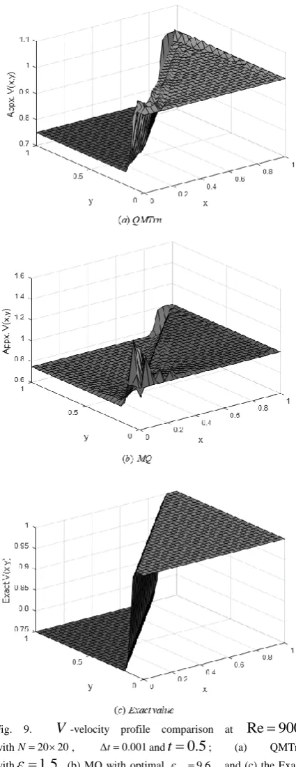
, (b) MQ with optimal opl9.6, and (c) the Exact profile.

Fig. 9.

V

-velocity profile comparison at

Re



900

withN20 20 ,  t 0.001and

t



0.5

; (a) QMTrn with





1.5

, (b) MQ with optimal opl9.6 , and (c) the Exact

profile.

IAENG International Journal of Applied Mathematics, 48:4, IJAM_48_4_17

[image:9.595.59.267.67.598.2] [image:9.595.320.533.235.786.2]





2

2

4 exp( 5 / Re) cos(2 ) sin( ) ( , , )

Re 2 exp( 5 / Re) sin(2 ) sin( )

t u x y t

t

   

  

  

  (41)





2

2

2 exp( 5 / Re) sin(2 ) cos( ) ( , , )

Re 2 exp( 5 / Re) sin(2 ) sin( )

t v x y t

t

   

  

  

  (42)

With

t



0

. And the initial conditions are;





4 cos(2 ) sin( ) ( , , 0)

Re 2 sin(2 ) sin( )

u x y   

 

 

 (43)





2 sin(2 ) cos( ) ( , , 0)

Re 2 sin(2 ) sin( )

v x y   

 

 

 (44)

This example is aimed to provide information on the CPU-time required in computation process when applying the method. Solutions shown in this Section presented in all tables are obtained using t 0.001. At the same optimal choice of shape parameter, Table 8 – 9 provide clear evidence that solutions obtained suing QMTrn and CMTrn stay in good agreement with the exact ones and are very close to those reported in the work of Aminikhah [42]. This trend is still also persistent when the Reynolds number increases to 500 and Matern type of RBF is found to over perform the MQ once, as shown in Table 10 – 11, with the change of the optimal shapeopl2.3, and even when the Reynolds number is as high as and even when the Reynolds number is as high as

Re 1,000



the good quality of solutions can still be obtained as illustrated in Fig 10 and Fig 11. With the increase of the number of nodes, as can be seen in Fig 12., Multiquadric RBF remain the cheapest choice in terms of CPT-time while the one that takes CPU-time to compute the same solution algorithm is seen to be QMTrn; with the difference of CPT-time between the two is approximately 250s at the same node density of 405 nodes.

TABLE VIII

SOLUTION COMPARISON OF

U

-VELOCITY COMPONENT ATRe 100, t0.5, USING N 9 9

Point

3.1 opl

 

Exact QMTrn CMTrn Ref.[42]

(0.1,0.1) -0.011460 -0.010860 -0.011401 -0.0114639

(0.5,0.1) 0.015170 0.015310 0.015110 0.0151741 (0.9,0.1) -0.013210 -0.013251 -0.013145 -0.0131984 (0.3,0.3) 0.009436 0.009954 0.009422 0.0094350 (0.7,0.3) 0.017548 0.017621 0.017512 0.0177710 (0.1,0.5) -0.032300 -0.031988 -0.032314 -0.0322795 (0.5,0.5) 0.049093 0.049102 0.049009 0.0490138 (0.3,0.7) 0.009436 0.009501 0.009452 0.0094350 (0.7,0.7) 0.017548 0.018520 0.017511 0.0177713 (0.1,0.9) -0.011460 -0.011504 -0.011562 -0.0114639 (0.5,0.9) 0.015170 0.015099 0.015140 0.0151741 (0.9,0.9) -0.013210 -0.013332 -0.013200 -0.0131984

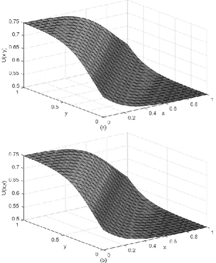
Fig. 10 Solution surface profile of U-velocity component at

Re1,000, t0.5,  t 0.001 using N20 20 and

3.25

 .

Fig. 11 Solution surface profile of V-velocity component at

Re1,000, t0.5,  t 0.001 using N20 20 and

3.25

 .

IAENG International Journal of Applied Mathematics, 48:4, IJAM_48_4_17

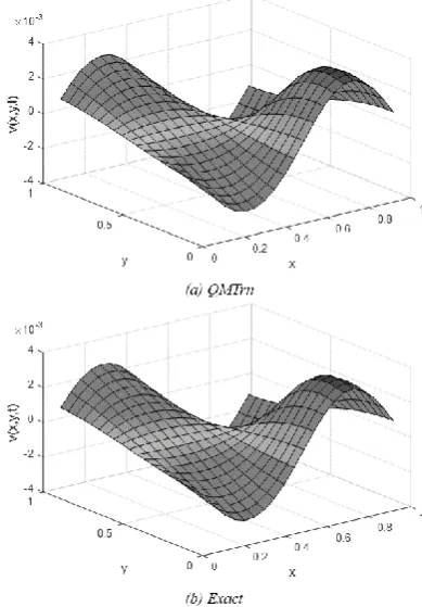
[image:10.595.46.290.77.220.2] [image:10.595.324.519.442.722.2] [image:10.595.51.291.560.784.2]

C. Example 3

This example deals with the 2D Burgers’ Equations with the initial conditions and boundary conditions are obtained directly from the exact solutions which are available in the work of Aminikhah [43] and Huazhong [44], expressed as;

2

2 ( , , )

1 2

x y xt u x y t

t

  

 (45)

2

2 ( , , )

1 2

x y yt v x y t

t

  

 (46)

The computational domain under the investigation is domain{( , ) : 0x y  x 0.5 , 0  y 0.5}. This final test case is expected to provide more information on the effects of the distribution of nodes as well as the effects of node density. In order to answer these questions, nodes are randomly distributed over the domain as depicted in Fig 13. while the measuring nodes are marked as shown in Table 12 - 13. In these two tables, the solutions agree well with both the exact and those provided by Huazhong [44], confirming the promising aspects of QMTrn and CMTrn.

When the number of nodes is increasing, Fig 14. clearly shows that MQ-RBF cannot be reliable when the errors are not clearly correlated with N. On the other hand, all three Metern RBFs are observed to be reducing while N is getting larger. The feature is mostly clear for the case of QMTrn and the L_rmserror norm is gradually decreasing with a lot less fluctuations while N is increasing, indicating the less sensitivity of accuracy to the node density.

V. CONCLUSION

A large number of numerical simulations have been carried out in this work aiming to explore in more details

TABLE IX

SOLUTION COMPARISON OF

V

-VELOCITY COMPONENT ATRe 100, t0.5, USING N 9 9

Point

3.1 opl

 

Exact QMTrn CMTrn Ref.[42]

[image:11.595.308.544.120.342.2]

(0.1,0.1) -0.012812 -0.012744 -0.012805 -0.0128133 (0.5,0.1) 0.000000 0.000015 0.000007 -0.0000071 (0.9,0.1) 0.014770 0.014699 0.014750 0.0147697 (0.3,0.3) -0.010550 -0.010485 -0.010599 -0.0105498 (0.7,0.3) 0.019619 0.019598 0.019684 0.0196916 (0.1,0.5) 0.000000 0.000095 0.000012 0.0000000 (0.5,0.5) 0.000000 0.000091 0.000009 0.0000000 (0.3,0.7) 0.010550 0.010651 0.010510 0.0105498 (0.7,0.7) -0.019614 -0.019501 -0.019599 -0.0199692 (0.1,0.9) 0.012812 0.012709 0.012958 0.0128133 (0.5,0.9) 0.000000 0.000095 0.000021 0.0000071 (0.9,0.9) -0.014770 -0.014110 -0.014797 -0.0147697

TABLE X

SOLUTION COMPARISON OF

U

-VELOCITY COMPONENT ATRe500,t0.5, USING N 9 9

Point

2.3 opl

 

Exact MQ-RBF CMTrn Ref.[42]

[image:11.595.55.285.298.540.2]

(0.1,0.1) -0.002752 -0.002102 -0.002706 -0.002752 (0.5,0.1) 0.003696 0.003002 0.003588 0.003696 (0.9,0.1) -0.003273 -0.003958 -0.003199 -0.003273 (0.3,0.3) 0.002188 0.002999 0.002104 0.002188 (0.7,0.3) 0.004718 0.005043 0.004701 0.004718 (0.1,0.5) -0.007561 -0.009021 -0.007555 -0.007561 (0.5,0.5) 0.011961 0.011055 0.011909 0.011961 (0.3,0.7) 0.002188 0.001125 0.002145 0.002188 (0.7,0.7) 0.004718 0.019502 0.004699 0.004718 (0.1,0.9) -0.002752 -0.008851 -0.002748 -0.002752 (0.5,0.9) 0.003696 0.005204 0.003608 0.003696 (0.9,0.9) -0.003273 -0.003802 -0.003266 -0.003273 Fig. 12: CPU-Time in seconds spent in each simulation at different nodes densities for Re 1, 200, t0.5 using t 0.001.

TABLE XI

SOLUTION COMPARISON OF

V

-VELOCITY COMPONENT AT Re500,t0.5, USING N 9 9

Point

2.3 opl

 

Exact MQ-RBF CMTrn Ref.[42]

(0.1,0.1) -0.003077 -0.003577 -0.003070 -0.003077 (0.5,0.1) 0.000000 0.000065 0.000008 0.000000 (0.9,0.1) 0.003659 0.003095 0.003645 0.003659 (0.3,0.3) -0.002447 -0.002996 -0.002439 -0.002447 (0.7,0.3) 0.005274 0.005305 0.005270 0.005274 (0.1,0.5) 0.000000 0.000601 0.000011 0.000000 (0.5,0.5) 0.000000 0.000551 0.000090 0.000000 (0.3,0.7) 0.002447 0.002559 0.002450 0.002447 (0.7,0.7) -0.005274 -0.005854 -0.005271 -0.005275 (0.1,0.9) 0.003077 0.003302 0.003081 0.003077 (0.5,0.9) 0.000000 0.000114 0.000009 0.000000 (0.9,0.9) -0.003659 -0.003551 -0.003664 -0.003659

IAENG International Journal of Applied Mathematics, 48:4, IJAM_48_4_17

the effectiveness of the so-called Radial Point Interpolation Method (RPIM). The method writes the approximate solution as a linear combination of a radial basis function (RBF), defining at each center node over the domain, together also with a polynomial function. Since

Multiquadric, the rather more popular choice of RBF, is

known to suffer from conditioning problem for the interpolation matrix, those in Matern category were focused on instead. To evaluate the method applied with Matern RBF, the famous nonlinear, transient and coupled-Burgers’ equations were tackled numerically. The results validation is performed using the corresponding exact ones and with also results published in literature when possible. Main findings achieved from this investigation can be listed as follows;

1) With the three forms of Matern RBF, it is found that the risk of encountering the ill-condition problem is notably reduced, giving more confidence when dealing with larger system of interpolation matrix

2) . At low Reynolds number, the method applied in this work is found to produce solutions with approximately the same level of accuracy as those documented in literature. It has to be noticed, however, that the number of degree of freedoms required are much less than other works indicating lower storage in CPU for computing.

3) At high Reynolds number, on the other hand, MQ-RBF can be a better choice in terms of CPU-time consumption, and yet in terms of accuracy CMTrn and QMTrn are still found to be superior.

4) When the inertial forces become more and more dominant, with an increase ofRe, Matern RBFs are witnessed to maintain the accuracy reasonably well while the MQ has a noticeable growth in error both for U-velocity and V-velocity components. 5) All three forms of Matern RBFs are clearly seen to

be much less sensitive to the change of the center nodes density. This is, however, not the case for MQ-RBF where the accuracy can be completely unreliable with higher nodes density.

6) The choice of shape parameter is found to have only an insignificant effect on the simulations done using Matern RBFs whereas a severe effect is found for the case of MQ-RBF.

[image:12.595.316.532.72.227.2]

7) Amongst only the three Materns, it is the Linear one that is found to produce comparatively worst results quality. Cubic and Quadratic are found to remain very close to each another in terms of accuracy and Fig. 13. Irregular node distribution with 100 computational nodes.

TABLE XII

COMPARISON OF COMPUTATIONAL U-SOLUTION AT

Re 1, t 0.1 WITH BOUNDARY NODES N 10 10

Point

2.8 opl

 

Exact QMTrn CMTrn Ref. [44]

(0.1,0.1) 0.183673 0.183605 0.183666 0.18368 (0.3,0.1) 0.346939 0.346911 0.346908 0.34694 (0.2,0.2) 0.367347 0.367369 0.367341 0.36735 (0.4,0.2) 0.530612 0.530606 0.530600 0.53062 (0.1,0.3) 0.387755 0.387711 0.387752 0.38776 (0.3,0.3) 0.551024 0.551018 0.551018 0.55103 (0.2,0.4) 0.571429 0.571420 0.571411 0.57144 (0.3,0.4) 0.653061 0.653058 0.653059 0.65307

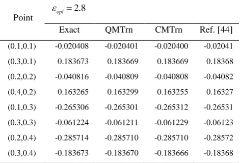
TABLE XIII

COMPARISON OF COMPUTATIONAL V-SOLUTION AT

Re 1, t 0.1 WITH BOUNDARY NODES N 10 10

Point

2.8 opl

 

Exact QMTrn CMTrn Ref. [44]

(0.1,0.1) -0.020408 -0.020401 -0.020400 -0.02041 (0.3,0.1) 0.183673 0.183669 0.183669 0.18368 (0.2,0.2) -0.040816 -0.040809 -0.040808 -0.04082 (0.4,0.2) 0.163265 0.163299 0.163255 0.16327 (0.1,0.3) -0.265306 -0.265301 -0.265312 -0.26531 (0.3,0.3) -0.061224 -0.061211 -0.061229 -0.06123 (0.2,0.4) -0.285714 -0.285710 -0.285710 -0.28572 (0.3,0.4) -0.183673 -0.183670 -0.183666 -0.18368

MQ-RBF

LMTrn QMTrn

[image:12.595.50.288.332.510.2]

CMTrn

Fig. 14: Average-RMS Error norm measured at a wide range of computational nodes with a fixed Re10.0 att0.5.

IAENG International Journal of Applied Mathematics, 48:4, IJAM_48_4_17

[image:12.595.52.288.558.718.2]

condition number over the whole range of Reynolds number under investigation.

To sum up, it is clearly seen that with all positive aspects discovered and presented in this work, Matern RBFs have revealed some promising Figs over the rather more popular choice of RBF such as Multiquadric. They, as a result, truly deserve further investigation and this shall remain one of our further numerical studies.

ACKNOWLEDGMENT

The corresponding author would like to express his sincere appreciation to the Center Of Excellence in Mathematics, Thailand, for their kind support.

REFERENCES

[1] Y. Deng, C. Liu, M. Peng and Y. Cheng, “The Interpolating Complex Variable Element-Free Galerkin Method for Temperature Field Problems,” International Journal of Applied Mechanics, vol. 07, no. 2, 2015.

[2] G.Y. Sheu, “Prediction of Probabilistic Settlements by the Perturbation-Based Spectral Stochastic Meshless Local Petrov– Galerkin Method,” Geotechnical and Geological Engineering, vol. 31, no. 5, 2013, pp. 1453-1464.

[3] B. Dai, B. Zheng, Q. Liang and L. Wang, “Numerical solution of transient heat conduction problems using improved meshless local Petrov–Galerkin method,” Applied Mathematics and Computation, vol. 219, no. 19, 2013, pp. 10044-10052.

[4] H. Gao, G. Wei, “Complex variable meshless manifold method for elastic dynamic problems,” Mathematical Problems in Engineering, 2016.

[5] E.J. Kansa, Multiquadrics—“A scattered data approximation scheme with applications to computational fluid-dynamics—II solutions to parabolic, hyperbolic and elliptic partial differential equations,” Computers & Mathematics with Applications, vol. 19, no. 8, 1990, pp. 147-161.

[6] G. Chandhini and Y. V. S. S. Sanyasiraju, “Local RBF-FD solutions for steady convection-diffusion problems,” International Journal for Numerical Methods in Engineering, vol. 72, no. 3, 2007, pp. 352-378.

[7] P.P. Chinchapatnam, K. Djidjeli, P.B. Nair, “Unsymmetric and symmetric meshless schemes for the unsteady convection–diffusion equation,” Computer Methods in Applied Mechanics and Engineering, vol. 195, no. 19, 2006, pp. 2432-2453.

[8] P.H. Wen and Y.C. Hon, “Geometrically nonlinear analysis of Reissner-Mindlin plate by Meshless computation,” CMES Computer Modeling Engineering Scences, vol. 21, 2004, pp. 177-191.

[9] H.J. Al-Gahtani, “RBF meshless method for large deflection of thin plates with immovable edges,” Engineering Analysis with Boundary Elements, vol. 33, no. 2, 2009, pp. 176-183.

[10] A.R. Ferreira, CMC; Martins, PALS, “Radial basis functions and higher-order shear deformation theories in the analysis of laminated composite beams and plates,” Composite structures, vol. 66, no. 1-4, 2001-4, pp. 287-293.

[11] K.M.L. Y. Liu, Y.C. Hon and X. Zhang, “Numerical simulation and analysis of an electroactuated beam using a radial basis function,” Smart Mater. Struct, vol. 14, no. 6, 2005, pp. 1163-1171.

[12] J. G. Wang and G. R. Liu, “A point interpolation meshless method based on radial basis functions,” International Journal for Numerical Methods in Engineering, vol. 54, no. 11, 2002, pp. 1623-1648. [13] X. Liu, G.R. Liu, K. Tai and K.Y. Lam, “Radial basis point

interpolation collocation method for 2-d solid problem,” Advances in Meshfree and X-FEM Methods, World Scientific, 2011, pp. 35-40.

[14] O.Y. Bozkurt, B.Kanber and M. Z. ASIk, “Assessment of RPIM shape parameters for solution accuracy of 2D geometrically monlinear problems,” Int. J. of Computational Methods, vol. 10, no. 3, 2013.

[15] M.B. H. Ghaffarzadeh, A. Mansouri. and M.H. Sadeghi, “Study of Meshfree Hermite Radial Point Interpolation Method for Flexural Wave Propagation Modeling and Damage Quantification,” Latin American Jounal of Solids and Sturctures, vol. 13, 2016, pp. 2606-2627.

[16] J. Ma, G. Wei, D. Liu and G. Liu, “The numerical analysis of piezoelectric ceramics based on the Hermite-type RPIM,” Applied Mathematics and Computation, vol. 309, 2017, pp. 170-182. [17] J.M. Burgers, “A Mathematical Model Illustrating the Theory of

Turbulence,” Advances in Applied Mechanics, vol. 11, 1948, vol. 171-199.

[18] J.a.J.D. Nee, “Limit Set of Trajectories of the Coupled Viscous Burgers Equations,” Applied Mathematics Letters, vol. 11, no. 1, 1998, pp. 57-61.

[19] S.E. Esipov, “Coupled Burgers equations: A model of polydispersive sedimentation,” Physical Review E, vol. 52, no. 4, 1995, pp. 3711-3718.

[20] D. Deng, and T. Pan, “A Fourth-order Singly Diagonally Implicit Runge-Kutta Method for Solving One-dimensional Burgers’ Equation,” IAENG International Journal of Applied Mathematics, vol. 45, no. 4, pp. 327-333, 2015.

[21] B. Wongsaijai, K. Poochinapan, and T. Disyadej, “A Compact Finite Difference Method for Solving the General Rosenau-RLW equation,” IAENG International Journal of Applied Mathematics, vol. 44, no. 4, pp. 192-199, 2014.

[22] S. Sungnul, B. Jitsom and M. Punpocha, “Numerical Solution of the Modified Burger’s equation using FTCS Implicit Scheme,” IAENG International Journal of Applied Mathematics, vol. 48, no. 1, pp. 53-61, 2018.

[23] A.R. Bahadır, “A fully implicit finite-difference scheme for two-dimensional Burgers-equations,” Appl. Math. Comput, vol. 137, 2003, pp. 131-137.

[24] M. Dehghan, A. Hamidi and M. Shakourifar, “The Solution of Coupled Burgers’ Equations using Adomain-Pade Technique,” Applied Mathematics and Computation, vol. 189, no. 2, 2007, pp. 1034-1047.

[25] A.A. Soliman, “On the Solution of Two-Dimensional Coupled Burgers’ Equations by Variational Iteration Method,” Chaos Solitions and Fractals, vol. 40, no. 3, 2009, pp. 1146-1155. [26] A. Ali, Siraj-ul-lslam and S. Haq, “A Computational Meshfree

Technique for the Numerical Solution of the Two-Dimensional Coupled Burgers’ Equations,” International Journal for Computational Methods in Engineering Science and Mechanics, vol. 10, no. 5, 2009, pp. 406-422.

[27] H. Zhu, H. Shu and M. Ding, “Numerical Solutions of Two-Dimensional Burgers’ Equations by Discreate Adomain Decomposition Method,” Computers and Mathematics with Applications, vol. 60, no. 3, pp. 840-848.

[28] S. Kaennakham, K. Chanthawara and W. Toutip, “Optimal Radial Basis Function (RBF) for Dual Reciprocity Boundary Element Method (DRBEM) applied to Coupled Burgers’ Equations with Increasing Reynolds Number,” Australian Journal of Basic and Applied Sciences, vol. 8, no. 7, 2014, pp. 462-476.

[29] K. Chanthawara, S. Kaennakham and W. Toutip, “The Dual Reciprocity Boundary Element Method (DRBEM) with Multiquadric Radial Basis Function for Coupled Burgers’ equations,” The International Journal of Multiphysics, vol. 8, no. 2, 2014, pp. 123-143.

[30] Y. Wang, I. M. Navon, X. Wang and Y. Cheng, “2D Burgers equation with large Reynolds number using POD/DEIM and calibration,” International Journal for Numerical Methods in Fluids, vol. 82, 2016, pp. 909-931.

IAENG International Journal of Applied Mathematics, 48:4, IJAM_48_4_17

[31] I.A. Cristescu, “Numerical resolution of coupled two-dimensional Burgers' equation,” Romanian Journal of Physics, vol. 62, 2017, pp. 103.

[32] M.L. Stein, Interpolation of Spatial Data: Some Theory for Kriging, New York: Springer-Verlag, 1999.

[33] C.A.J. Fletcher, “Generating Exact Solutions of the Two-Dimensional Burgers equations,” International Journal for Numerical Methods in Fluids, vol. 3, no. 3, 1983, pp. 213-216. [34] C. Gaspar, “Multi-level meshless methods based on direct

multi-elliptic interpolation,” Journal of Computational and Applied Mathematics, vol. 226, no. 2, 2009, pp. 259-267.

[35] C.F. D. Younga, S. Hua and S. Atluri, “The Eulerian–Lagrangian method of fundamental solutions for two-dimensional unsteady Burgers’ equations,” Eng.Anal. Bound Elem, vol. 32 2009, pp. 395-412.

[36] M. Mohammadi, R. Mokhtari and H. Panahipour, “A Galerkin-reproducing kernel method: Application to the 2D nonlinear coupled Burgers' equations,” Engineering Analysis with Boundary Elements, vol. 37, no. 12, 2013, pp. 1642-1652.

[37] I. Siraj ul, B. Šarler, R. Vertnik and G. Kosec, “Radial basis function collocation method for the numerical solution of the two-dimensional transient nonlinear coupled Burgers’