Compositional Modeling of Two-Phase Flow in Porous Media Using Semi-Implicit Scheme

Compositional Modeling of Two-Phase Flow in

Porous Media Using Semi-Implicit Scheme

Ondˇrej Pol´ıvka and Jiˇr´ı Mikyˇska

Abstract—In this paper we deal with the numerical modeling of the compressible two-phase flow of a mixture composed of several components in porous media with species transfer between the phases. We formulate the mathematical model by means of the extended Darcy’s laws for all phases, components continuity equations, constitutive relations, and appropriate initial and boundary conditions. The splitting of components among the phases is described by a formulation of the local thermodynamic equilibrium which uses volume, temperature, and moles as specification variables. We solve the problem numerically using a combination of the mixed-hybrid finite element method for the total flux discretization and the finite volume method for the discretization of transport equations, and the semi-implicit time discretization. The proposed numer-ical flux approximation does not require phase identification and determination of the corresponding phases on adjacent elements. The resulting system of nonlinear algebraic equations is solved by the Newton-Raphson method. In contrast to fully-implicit schemes, the size of the final system does not depend on the number of mixture components.

Index Terms—semi-implicit phase-by-phase upwinding, mixed-hybrid finite element method, finite volume method, constant-volume phase splitting.

I. INTRODUCTION

M

ATHEMATICAL modeling of gas injection into oil reservoirs is important in dealing with problems like enhanced oil recovery or CO2sequestration. The mathemat-ical model has to describe transport of a mixture composed of several chemical components in a porous medium. De-pending on the local thermodynamic conditions, the mixture can remain in a single phase or can split into two (or more) phases.

In this paper, we follow our previous work [14], where we have derived a fully-implicit numerical scheme for the compositional modeling in which components splitting among the phases is described by a formulation of the local thermodynamic equilibrium at constant volume, temperature, and moles (V T-flash) [11], [12], [6], [7]. The fully-implicit scheme is stable allowing for long time steps, but it suffers from higher computational costs because a large system of equations has to be solved. Moreover, the size of the final system is proportional to the number of mixture components.

Manuscript received December 31, 2013; revised July 21, 2014. This work was supported by the project P105/11/1507 Development of Computational Models for Simulation of CO2 Sequestration of the Czech Science Foun-dation and by the project KONTAKT II LH 12064 Computational Methods in Thermodynamics of Hydrocarbon Mixtures of the Ministry of Education, Youth and Sport of the Czech Republic.

O. Pol´ıvka is with the Department of Mathematics, Faculty of Nu-clear Sciences and Physical Engineering, Czech Technical University in Prague, Trojanova 13, 120 00 Prague 2, Czech Republic, e-mail: [email protected]

J. Mikyˇska is with the Department of Mathematics, Faculty of Nu-clear Sciences and Physical Engineering, Czech Technical University in Prague, Trojanova 13, 120 00 Prague 2, Czech Republic, e-mail: [email protected]

A remedy for this disadvantage could be an explicit scheme, where one does not have to solve any system. However, explicit schemes are conditionally stable with very restrictive size of the time step. We propose a semi-implicit approach based on a combination of the mixed-hybrid finite element method (MHFEM) and the finite volume method (FVM). Similarly to the fully-implicit schemes, our method leads to large systems of linear algebraic equations, but it is possible to reduce the size of the final system of equations to a size independent of the number of mixture components. Therefore, the size of the final linear system is significantly reduced which is a desirable feature, especially for mixtures composed of a large number of components.

The paper is structured as follows. In Section II, the mathematical model is formulated by means of partial differ-ential equations representing the conservation laws, Darcy’s laws, and by means of the conditions of local thermody-namic equilibrium in the V T-settings. Several fluxes are introduced and some important relations between them are described. Then, the compositional model is formulated and appropriate initial and boundary conditions are prescribed. In Section III, the system of equations is solved numerically using the MHFEM for Darcy’s law discretization, and the FVM including upwind technique for the components trans-port equations discretization. The semi-implicit scheme is derived and linearized using the Newton-Raphson iterative method (NRM), and the system of equations is reduced to a size that is independent of the number of components. In Section IV, the basic steps of the computational algorithm are summarized. Examples of computations using the semi-implicit approach and comparisons of results with the fully-implicit approach are presented in Section V. In Section VI, essential features of the method are commented and some conclusions are drawn. In Appendix, details on the equation of state used in the calculation are provided.

II. MODELEQUATIONS

A. Transport Equations

Consider two-phase compressible flow of a mixture com-posed ofnc components in a porous medium with porosity φ[-] at a constant temperatureT [K]. If we neglect diffusion and capillarity, the transport of the components can be described by the following molar balance equations [10], [14]

∂(φci) ∂t +∇ ·

X

α

cα,ivα

!

=Fi, i= 1, . . . , nc, (1)

where P

α sums over all phases, ci is the overall molar

concentration of componenti [mol m−3], cα,i is the molar

concentration of componentiin phaseα[mol m−3], andFi

is the sink or source term [mol m−3s−1]. The phase velocity

IAENG International Journal of Applied Mathematics, 45:3, IJAM_45_3_07

vα is given by the extended Darcy’s law vα=−λαK(∇p−%αg), λα=

krα µα

, (2)

whereK=K(x)is the medium intrinsic permeability [m2],

pis the pressure [Pa], %α =P nc

i=1cα,iMi is the density of

fluid in phase α (Mi is the molar weight of component i

[kg mol−1]), and g is the gravitational acceleration vector [m s−2]. The α-phase mobility λα is given by the ratio

of the α-phase relative permeability krα [-] and α-phase

dynamic viscosityµα[kg m−1s−1]. The relative permeability

and dynamic viscosity depend on properties of phase αas

krα=krα(Sα), µα=µα(T, cα,1, . . . , cα,nc), (3) where Sα is the saturation of phase α and viscosity is

computed using the Lohrenz-Bray-Clark method [9].

B. Phase Computations

As we study generally the two-phase flow, a mixture can stay in the single phase or two phases at each point. To decide on the number of phases from temperature T > 0

and overall molar concentrations c1, . . . , cnc, we use the constant volume phase stability test described in [12]. In the single-phase case, cα,i=ci, Sα = 1 hold, and pressure is

given by the Peng-Robinson equation of state (detailed in Appendix) of the form

p=p(T, c1, . . . , cnc). (4) If the V T-stability indicates that the system is in two phases, the splitting of components among the phases is given by the following phase equilibrium conditions [11]

X

α

cα,iSα=ci,

X

α

Sα= 1, (5a)

∀α6=β , ∀i= 1, . . . , nc,

p(T, cα,1, . . . , cα,nc) =p(T, cβ,1, . . . , cβ,nc), (5b) e

µi(T, cα,1, . . . , cα,nc) =µei(T, cβ,1, . . . , cβ,nc). (5c) Equations (5) express the balance of mass and volume (5a), mechanical equilibrium (5b), and chemical equilibrium (5c) in which µ_ei denotes the chemical potential of component i,

which can be derived from the equation of state. The exact form of µ_ei for the Peng-Robinson equation of state can be

found in [6], [11], [12].

The system of2·nc+ 2equations (5) for unknown molar

concentrations of all components in both phases cα,i and

phase saturationsSα can be solved by the Newton-Raphson

method (for details see [11]). Then, the equilibrium pressure

pcan be determined using the equation of state as

p=p(T, cα,1, . . . , cα,nc), (6) whereαis any of the split-phases.

C. Introduction of Fluxes

For the derivation of the numerical scheme, we need to define several fluxes. We denote qα,i the i-th component

flux in phaseα,qi the i-th component total flux, andqthe

total flux given by

qα,i=cα,ivα, (7a)

qi=

X

α

qα,i=

X

α

cα,ivα, (7b)

q=X

i qi=

X

α

cαvα, (7c)

wherecα=P nc

i=1cα,iis the totalα-phase concentration. By

substituting (2) into (7c), we can formulate Darcy’s law for the total flux as

q=−X

α

cαλαK(∇p−e%g), (8)

where

e

%=

P

αcαλα%α

P

αcαλα

(9) is an average density. Then, using (7a), (8), and (2),qα,ican

be evaluated as

qα,i=

cα,iλα

P

βcβλβ

 q−

X

β

cβλβ(%β−%α)Kg

 , (10) and, consequently, the total component flux is given from (7b) as

qi=

X

α

cα,iλα

P

βcβλβ

 q−

X

β

cβλβ(%β−%α)Kg

 .

(11)

D. Mathematical Formulation

LetΩ⊂Rd(d∈N) be a bounded domain andIbe a time

interval. In Ω×I, we solve for ci =ci(x, t) the following

equations which can be obtained from the transport equations (1) and (7b)

∂(φci)

∂t +∇ ·qi=Fi, i= 1, . . . , nc, (12)

whereqi is given by (11), andqis given by (8). The molar

concentrationscα,iand saturations are related to the overall

molar concentrationsciby (5) from which we also determine

the pressure (see Section II-B). Relative permeabilities and viscosities are given by (3). For this system of equations, we impose the following initial and boundary conditions

ci(x,0) =c0i(x), x∈Ω, i= 1, . . . , nc, (13a) p(x, t) =pD(x, t), x∈Γp, t∈I , (13b) qi(x, t)·n(x) = 0, x∈Γq, t∈I , i= 1, . . . , nc,

(13c) wherenis the unit outward normal vector to the boundary

∂Ω, Γp∪Γq = ∂Ω, and Γp∩Γq = ∅. Initial values of

molar concentrations are given by (13a), whereas (13b) is the Dirichlet boundary condition prescribing the pressurepD

onΓp, and (13c) is the zero Neumann boundary condition

representing impermeable boundary onΓq. We assume that Γp is the outflow boundary, so no boundary condition for

concentration has to be imposed.

IAENG International Journal of Applied Mathematics, 45:3, IJAM_45_3_07

III. NUMERICALMODEL

The system of equations (12), (5), and (13) is solved numerically using a combination of the MHFEM for the total flux discretization, and the FVM for the transport equations discretization. The obtained system is linearized by the NRM. The number of phases is determined locally on every element using the stability algorithm described in [12] at constant temperature and overall molar concentrations. In two-phase elements, the splitting of components among the phases is computed from theV T-flash algorithm [11]. Once the phase splitting is computed, pressure is evaluated readily using the equation of state.

We consider a 2D polygonal domainΩwith the boundary

∂Ωwhich is covered by a conforming triangulationTΩ. We denoteK the element of the meshTΩwith area|K|,E the edge of an element with the length |E|, nk the number of

elements of the triangulation, andnethe number of edges of

the mesh.

A. Discretization of Darcy’s Law for the Total Flux

The total flux q is approximated locally in the Raviart-Thomas space of the lowest order (RT0(K)) over the element

K∈ TΩ [2], [14], [10] as

q|K =

X

E∈∂K

qK,EwK,E, (14)

where the coefficient qK,E represents the numerical flux of

vector functionqthrough the edgeEon the elementKwith respect to the outer normal, and wK,E is the basis function

of RT0(K)associated with the edgeE. The basis functions are given by

wK,E(x) = 1

2|K|(x−NK,E), ∀x∈K , E∈∂K , (15) where NK,E ∈ K is a node against edge E. The basis

functions (15) satisfy the following properties ∇ ·wK,E(x) =

1

|K|, wK,E(x)·nK,E0 =

δE,E0

|E| . (16) Using (16) and techniques described in [14], we derive the mixed-hybrid finite element discretization of Darcy’s law for the total flux (8) as

qK,E =

X

α∈Π(K)

cα,Kλα,K αKEpK−

− X

E0_∈∂K βK_E,E0

b

pK,E0+γ_EK

e

%K

!

, E∈∂K, (17) where the coefficients are given by

αK_E = X E0_∈∂K

A−_K,E,E1 0, β_E,EK 0 =A−_K,E,E1 0,

γKE =

X

E0_∈∂K

A−_K,E,E1 0GK,E0,

(18)

where A−_K,E,E1 0 is an element of the inverse matrix A−

1

K , AK = (AK,E,E0)

E,E0_∈∂K ,and AK,E,E0 =

Z

K

K−1wK,E·wK,E0, G_K,E0 =

Z

K

g·wK,E0.

(19)

In (17),Π(K)is set of all phases on elementK,pK denotes

the cell pressure average,_bpK,E0 is the edge pressure average, cα,K, λα,K,%_eK are the mean values of concentration and

mobility of phase α, and average density on element K. The cell-averaged quantities are functions of the overall molar concentrations and temperature at element K; their evaluation is described in Section III-C.

In the mixed-hybrid formulation, we require the continuity of total flux normal component and pressure on the edgeE

between neighboring elements K, K0 ∈ TΩ which can be formulated as

qK,E+qK0_,E = 0, (20)

b

pK,E =pbK0,E =:pbE. (21) The boundary conditions (13b), (13c) are discretized as

b

pE =pD(E), ∀E⊂Γp, (22a) qK,E = 0, ∀E, K :E⊂Γq, E∈∂K , (22b)

wherepD_{(E)is the prescribed value of pressurep}D_averaged

on the edgeE.

We can eliminate the numerical fluxqK,E by substituting

from (17) into (20) and (22b). For further derivation, let us consider time dependent quantities at timetn+1 denoted by upper indexn+1. Then, Equations (17)–(22) transform to the following system ofne linear algebraic equationsFE = 0,

where

FE=

            

P

K:E∈∂K

P

α∈Π(K)

cn_α,K+1λn_α,K+1

!

αK Ep

n+1

K −

− P

E0_∈∂K β_E,EK 0p_b

n+1

E0 +γ_EK%_e n+1

K

, ∀E6⊂Γp,

b

pn_E+1−pD(E), ∀E⊂Γp.

(23) Herein, the symbol P

K:E∈∂K denotes the sum over the

elements adjacent to the edgeE .

B. Discretization of the Transport Equations

For the discretization of the transport equations (12) with the initial and boundary conditions (13), similarly as in [14], we use the FVM [8]. Unlike in [14], where the fully-implicit scheme was derived, here, we derive the semi-implicit scheme. Integrating (12) over an arbitrary element

K∈ TΩand using Green’s theorem, we have

d dt

Z

K

φ(x)ci(x, t) +

Z

∂K

qi(x, t)·n∂K(x) =

Z

K

Fi(x),

i= 1, . . . , nc. (24)

Applying the mean value theorem on (24), and de-noting φK, ci,K, Fi,K, the averaged values of φ, ci, Fi (i= 1, . . . , nc) over the cell K, respectively, the

semi-discrete form of (12) reads as

d(φKci,K) dt |K|+

X

E∈∂K

qi,K,E =Fi,K|K|, (25)

whereqi,K,E is a numerical approximation of

R

Eqi·nK,E

for E ∈ ∂K. To evaluate the numerical flux qi,K,E, we

IAENG International Journal of Applied Mathematics, 45:3, IJAM_45_3_07

propose the following upwind technique

qi,K,E=

               P

α∈Π(K,E)+

qα,i,K,E − P β∈Π(K0_,E)+

qβ,i,K0_,E,

∀E /∈∂Ω,

P

α∈Π(K,E)+

qα,i,K,E, ∀E∈Γp, 0, ∀E∈Γq,

(26) where Π(K, E)+ _{= {α∈Π(K)|q}

α,i,K,E>0} for E ∈ ∂K , andqα,i,K,E is given by

qα,i,K,E=

cα,i,Kλα,K

P

β∈Π(K)

cβ,Kλβ,K

(qK,E−

− X

β∈Π(K)

cβ,Kλβ,K(%β,K−%α,K)γEK

 . (27) Notice that (26) is an approximation of (11), and (27) is a discrete form of (10). In (26), we sum only over the outflowing phases through the edgeE. This method ensures that no phase identification or phase interconnection between neighboring elements is necessary, and the total component fluxes are balanced on each inner edge. In (27) qK,E is

given by (17), cα,i,K and Sα,K are computed locally on

each element byV T-flash (see Section II-B), and from them,

cα,K, λα,K, and%α,K are evaluated.

Assuming that the porosity does not depend on time, the time derivative ofci,K in (25) is approximated by the time

difference with a time step∆tn. For everyn ,allK∈ TΩ,

and i= 1, . . . , nc the semi-implicit scheme can be derived

from Equation (25) in a form FK,i= 0,where

FK,i=φK|K|

cn_i,K+1−cn i,K

∆tn

+ X

E∈∂K

q_i,K,En+1/2−Fi,K|K|,

(28) whereqn_i,K,E+1/2 is given by (26) using

qn_α,i,K,E+1/2 = c n

α,i,Kλnα,K

P

β∈Π(K)n cn

β,Kλ n β,K

qn_K,E+1−

− X

β∈Π(K)n

cn_β,Kλn_β,K %n_β,K−%n_α,K

γ_EK

 . (29) Note that onlyq_K,En+1is taken from the new time level in (29), all other terms are given explicitly from the previous time level includingΠ(K)n_{which denotes phases on elementK}

at time level n. This is the key point enabling to reduce the system of equations to a size that is independent of the number of mixture components described in the next section.

The initial conditions (13a) are approximated as

c0i,K=c0i(K), ∀K∈ TΩ, i= 1, . . . , nc, (30)

wherec0

i(K)denotes the average value ofc0i on elementK.

C. Assembling the Final System

In Equations (23) and (28), we have denotedFEandFK,i,

(for the edge E ∈ {1, . . . , ne}, element K∈ {1, . . . , nk},

and component i∈ {1, . . . , nc}) the expressions which

rep-resent the components of a vectorF. To evaluate quantities

cα,K, λα,K, %eK contained in (23) and also other element-averaged functions depending on the phase splitting, we performV T-flash calculation on element K using the cell-averaged values cn_1,K+1, . . . , cn_n+1

c,K and temperature T. The cell-averaged pressure pn_K+1 is also given implicitly by the result of theV T-flash and by (6) as

p_Kn+1=pT, c_α,n+1_1,K, . . . , cn_α,n+1 c,K

. (31)

This relation is valid in both single- and two-phase states due to (5b). We therefore solve a nonlinear system of algebraic equations ofnk·nc+ne equations

F1= [F1,1, . . . ,Fnk,nc] T

=0

F2= [F1, . . . ,Fne] T

=0 (32)

for unknown primary variables – overall molar concentra-tions cn_1,K+1, . . . , cn_n+1

c,K, K ∈ {1, . . . , nk}, and pressures on the edges_bpn_E+1, E∈ {1, . . . , ne}.

To solve (32), we use the NRM [16]. In each iteration of the NRM, we need to solve the following system of linear algebraic equations

J11 J12

J21 J22

δc δp_b

=

−F1 −F2

. (33)

The Jacobian matrix of system (33) composed of blocks

J11, . . . ,J22 is sparse and nonsymmetric. Elements of the matrix can be evaluated analytically using the following relations

(J11)K,i;K0_,j = ∂FK,i ∂cn_j,K+10

, (J12)K,i;E= ∂FK,i ∂p_bn_E+1,

(J21)E;K,j= ∂FE

∂cn_j,K+1, (J22)E,E0 = ∂FE ∂p_bn_E+10

, (34)

where i, j = 1, . . . , nc; K, K0 = 1, . . . , nk; E, E0 = 1, . . . , ne. The vectors of solutions δc and δpbcontain the corrections of nk ·nc molar concentrations δcni,K+1 and ne

pressures on the edges δp_bn_E+1,which are computed in each NRM-iteration and added to the values of cn_i,K+1 and _bpn_E+1

given from the previous iteration. The iteration procedure ends when the condition

kFk< ε (35)

is satisfied for a chosenε >0 [16].

The proposed semi-implicit scheme allows to reduce the size of system (33). By evaluatingqK0_,E from (20) and

sub-stituting it intoqβ,i,K0_,E in (26), matrixJ₁₁becomes

block-diagonal, each block being anc×nc matrix corresponding

to a single element. Then, by inverting the diagonal blocks,

J21 can be eliminated and (33) transforms to _J

11 J12

0 J22−J21(J11)−1J12

δc δp_b

=

=

−F1

J21(J11)

−1

F1−F2

. (36) Then, the system can be reduced to the final system

h

J22−J21(J11)− 1

J12 i

δp_b=

=J21(J11)

−1

F1−F2, (37)

IAENG International Journal of Applied Mathematics, 45:3, IJAM_45_3_07

for unknowns δp_bn_E+1, E = 1, . . . , ne. Thus, we eliminated

the internal degrees of freedomδcn_i,K+1, i= 1, . . . , nc, K= 1, . . . , nk,which are subsequently computed from (36) using

the evaluated inversion ofJ11 as

δc=−(J11)

−1

(F1+J12δpb). (38) The procedure of reducing the system in (33) to (37) is similar to static condensation described in [2]. The inversion of J11 is possible since the matrix is diagonally dominant for small time steps, and can be computed in parallel by inverting diagonal blocks inJ11.

The robustness of the NRM is increased by using the line-search technique [16] which ensures decreasing of kFk in each NRM-iteration with respect to the previous iteration. If the NRM cannot converge in 20 iterations, the time step is restarted and the value∆tnis halved. If the NRM converges

in less than 5 iterations, the time step is accepted and the next time step size is increased (∆tn+1= 1.2∆tn).

In contrast to the fully-implicit approach in [14], where it was necessary to solve a system of size (nc · nK + nE)×(nc·nK+nE)as in (33), here in the semi-implicit

approach, the size of the final system (37) isnE×nE,which

does not depend on the number of mixture components. The linearization is performed with respect to the persistent variables – i.e. well defined independently of whether a given element is in a single phase or two phases. The derivatives in (34) are also well defined in both single phase and two phases. Therefore, our schemes here and in [14] perform well in both cases and no primary variables switching is needed for treating phase appearance/disappearance (cf. [3], [4], [15]). As the discretization of the transport equations is based on the approximation of the total component flux, the connection between the elements with different number of phases is treated in a natural way.

IV. ALGORITHM

The computation proceeds in the following steps: 1) Initialize the geometry, physical and chemical

param-eters, and molar concentrations, generate a domain triangulation. Compute αK_E, β_E,EK 0, and γ_EK for all

elements and their edges.

2) Calculate pressures pK on each element using the

equation of state (4) and initial molar concentrations, then initialize all edge pressuresp_bE by averaging pK

on neighboring elements.

3) Repeat until the predetermined final time is reached

(tn∈I):

a) Repeat the NRM-iterations until the convergence criterion (35) is satisfied:

i) Perform the stability and flash calculations (see Section II-B) to obtain a number of phases and their compositions locally on all elements.

ii) For eachK, compute the cell-averaged pres-surespn_K+1 using (31), and average densities e

%n_K+1 using (9).

iii) Evaluate the total fluxes q_K,En+1 using (17), and phase fluxes q_α,i,K,En+1/2 using (29) and the quantities from the previous time step.

10 20 30 40 50

y

[

m

]

10 20 30 40 50

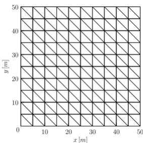
[image:5.595.348.490.62.204.2]

x[m] 0

Fig. 1. Structure of the computational grid.

iv) Assemble and solve system (37) for correc-tions of pressuresδp_bn_E+1.

v) From (38) compute corrections of molar con-centrationsδcn_i,K+1usingJ−₁₁1computed in the previous step.

vi) Add correctionsδcn_i,K+1andδp_bEn+1tocn_i,K+1and b

pn_E+1, respectively, check the convergence criterion (35).

b) Evaluate λn_α,K+1 and%n_α,K+1 on each element for all present phases.

c) Continue to the next time level (n→n+ 1). In step 2), only single phase is considered. In steps i. and ii., number of phases, their compositions, and pn_K+1 are computed using the data from the last available Newton iteration. In the first iteration, data from the previous time step are used.

V. RESULTS

In this section, we present numerical results of compo-sitional simulations of carbon dioxide (CO2) injection into reservoirs filled with different mixtures at constant temper-ature. The results have been computed using the numerical scheme described in Section III. We have computed the flow in a 2D square reservoir50×50m2 with porosity φ= 0.2

and isotropic permeability K = k = 9.87·10−15m2 (i.e. 10 mD). Structure of the computational grid consisting of

200 elements is shown in Fig. 1. Parameter ε from the NRM-convergence criterion (35) has been chosen10−6 _for all computations. The systems of linear algebraic equations have been solved using the direct solver UMFPACK [17], [18], [19], [20]. All examples have been computed on a grid of3200elements. In each figure, isolines of the overall molar fractionci/(Pn_i=1c ci)are depicted, and the two-phase region

is represented by gray color. We also mention the average time steps (computed as arithmetic mean from 5 values at time levels: 0.32, 0.63, 0.95, 1.27, and 1.58years) and CPU times using the current scheme and the fully-implicit scheme [14] in every example. All simulations have been computed on Six-Core AMD Opteron(tm) Processor 2427 at 2.2 GHz and 32 GB memory. Only V T-flash calculations were performed in parallel. The rest of the computation was sequential.

IAENG International Journal of Applied Mathematics, 45:3, IJAM_45_3_07

10 20 30 40 50

y

[

m

]

10 20 30 40 50 x[m]

0 Injection

of CO2

Outflow of mixture

[image:6.595.300.551.50.312.2]

Subsurface reservoir originally filled with propane or oil

Fig. 2. Outline of the simulated reservoir.

TABLE I

RELEVANT PARAMETERS OF THEPENG-ROBINSON EQUATION OF

STATE(40)FOREXAMPLES1AND2. VOLUME TRANSLATION IS NOT

USED.

i(component) pci[MPa] Tci[K] Vci[m3mol−1]

1(CO2) 7.375 304.14 9.416·10−5

2(C3) 4.248 369.83 2·10−4

i(component) Mi[g mol−1] ωi[-] δi1 [-] δi2 [-]

1(CO2) 44 0.239 0 0.15

2(C3) 44.0962 0.153 0.15 0

A. Injection of Carbon Dioxide into Propane Reservoir

Let us consider a cut through a reservoir filled with liquid propane (C3) at initial pressurep= 2.5MPa and temperature

T = 311K. In the left bottom corner of the reservoir, gaseous CO2 is injected, and in the right upper corner, the mixture of CO2 and propane is produced (Fig. 2). The injection rate of CO2 is 1778.1 mol/day. The parameters of the Peng-Robinson equation of state for both components of the mixture are summarized in Table I. In these settings, both CO2 and propane are single-phase but when mixed, the mixture can split into two phases. The boundary of the domain is impermeable except for the outflow corner where pressure p = 2.5MPa is maintained. Relative permeability depends linearly on saturation as krα(Sα) = Sα for each

phaseα.

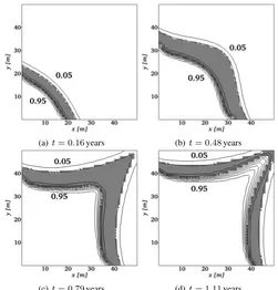
Example 1: In Fig. 3, a simulation of CO2 injection into a horizontal reservoir originally filled with propane is shown at four different times. Isolines of CO2overall molar fraction are distributed uniformly between the two displayed values of 0.9 and 0.1. The mixture stays in the single phase in the majority of the domain, only in the zone where the molar fractions are greater than 0.1 and less than 0.9, the two-phase region (colored in gray) appears. In comparison with results of the fully-implicit scheme [14], the contours of CO2overall molar fraction are almost the same. The average time step is 153minutes for the semi-implicit scheme and

179minutes for the fully-implicit scheme. The computation to t = 1.58years lasted 8.9hours using the semi-implicit scheme and9.4hours using the fully-implicit scheme.

(a)t= 0.16years (b)t= 0.48years

[image:6.595.67.274.54.246.2]

(c)t= 0.79years (d)t= 1.11years

Fig. 3. Isolines of CO2 overall molar fraction and the two-phase region (gray color) at different times. Contours are distributed uniformly between the two printed values. The solution is computed on a grid of3200elements: Example 1.

Example 2: In this example, we simulate the CO2injection into a vertical propane reservoir. So the only difference between this and the previous example is the non-zero gravity here. Uniformly distributed contours of CO2 overall molar fraction between 0.9 and 0.1 are visualized in Fig. 4. The single-phase mixture occupies a major part of the domain during the simulation but in the mixing zone a two-phase do-main also develops. At timet= 0.55years, we observed the maximum number of two-phase elements during the whole simulation. Afterwards, the number of two-phase elements decreases. In comparison with the fully-implicit scheme [14], the results almost coincide, and the average time steps are

141minutes (the current scheme) and280minutes (the fully-implicit scheme). The computation to t= 1.58years lasted

51.6hours using the semi-implicit scheme and 10.4hours using the fully-implicit scheme.

B. Injection of Carbon Dioxide into Oil Reservoir

Let us consider a cut through an oil (8-component hydro-carbon mixture) reservoir at initial pressure p= 2.76MPa and temperature T = 403.15K. The initial overall molar fractions of the oil components in the reservoir are written in Table II. Gaseous CO2 is injected in the left bottom corner of the reservoir, and the mixture of CO2 and oil is produced in the right upper corner. The injection rate of CO2 is 5578.2 mol/day. The reservoir is outlined in Fig. 2. The parameters of the Peng-Robinson equation of state for all components of the mixture are summarized in Table III. In these settings, the mixture can stay in the single phase or two phases. The boundary of the domain is impermeable except for the outflow corner where pressurep= 2.76MPa is maintained. Relative permeability depends quadratically on saturation askrα(Sα) =Sα2 for each phaseα.

IAENG International Journal of Applied Mathematics, 45:3, IJAM_45_3_07

TABLE III

RELEVANT PARAMETERS OF THEPENG-ROBINSON EQUATION OF STATE(40)FOREXAMPLES3AND4. VOLUME TRANSLATION IS NOT USED.

i(component) pci[MPa] Tci[K] Vci[m3mol−1] Mi[g mol−1] ωi[-]

1(CO2) 7.375 304.14 9.416·10−5 _{44 0.239}

2(N2) 3.39 126.21 8.988·10−5 _{28 0.039}

3(C1) 4.599 190.56 9.84·10−5 _{16 0.011}

4(C2–C3) 4.654 327.81 1.6571·10−4 _{34.96 0.11783}

5(C4–C5) 3.609 435.62 2.7522·10−4 _{62.98 0.21032}

6(C6–C10) 2.504 574.42 4.6839·10−4 _{110.21 0.41752}

7(C11–C24) 1.502 708.95 9.3876·10−4 _{211.91 0.66317}

8(C25+) 0.76 891.47 1.9298·10−3 _{462.79 1.7276}

i(component) δi1[-] δi2[-] δi3 [-] δi4 [-] δi5[-] δi6[-] δi7[-] δi8 [-]

1(CO2) 0 0 0.15 0.15 0.15 0.15 0.15 0.08

2(N2) 0 0 0.1 0.1 0.1 0.1 0.1 0.1

3(C1) 0.15 0.1 0 0.0346 0.0392 0.0469 0.0635 0.1052

4(C2–C3) 0.15 0.1 0.0346 0 0 0 0 0

5(C4–C5) 0.15 0.1 0.0392 0 0 0 0 0

6(C6–C10) 0.15 0.1 0.0469 0 0 0 0 0

7(C11–C24) 0.15 0.1 0.0635 0 0 0 0 0

8(C25+) 0.08 0.1 0.1052 0 0 0 0 0

(a)t= 0.16years (b)t= 0.48years

(c)t= 0.79years (d)t= 1.11years

Fig. 4. Isolines of CO2 overall molar fraction and the two-phase region (gray color) at different times. Contours are distributed uniformly between the two printed values. The solution is computed on a grid of3200elements: Example 2.

Example 3: In Fig. 5, a simulation of CO2injection in the left bottom corner of a horizontal reservoir originally filled with oil is shown. In the right upper corner, the mixture is produced. In each of the 8 plots, isolines of the overall molar fractions are visualized for every component at time

TABLE II

THE INITIAL OVERALL MOLAR FRACTIONS IN THE RESERVOIR FOR

EXAMPLES3AND4.

Component CO2 N2 C1 C2–C3

Overall molar fraction 0.0086 0.0028 0.4451 0.1207

Component C4–C5 C6–C10 C11–C24 C25+

Overall molar fraction 0.0505 0.1328 0.1660 0.0735

t= 1.36years. Contours are distributed uniformly between the displayed values. In each figure the two-phase region is colored in gray color. In comparison with Examples 1 and 2, the two-phase region occupies a major part of the domain (not only the part between 0.9 and 0.1 contours of CO2 molar fraction). If we compare the simulations from the semi-implicit and fully-implicit schemes, we obtain almost identical results. We have measured the average time step133minutes and 347minutes for the semi-implicit and fully-implicit schemes, respectively. The computation to t = 1.58years lasted 70.9hours using the semi-implicit scheme and66.9hours using the fully-implicit scheme.

Example 4: This example is similar to Example 3, but this time we simulate injection of CO2 into a vertical oil reservoir. CO2 is injected in the left bottom corner and the mixture is produced in the right upper corner. Results of the simulation at timet= 1.36years are shown in Fig. 6 using the isolines of the overall molar fractions of each component. The two-phase region is colored in gray in each figure. As in Example 3, also here, the two-phase region occupies a significant part of the reservoir. The semi-implicit scheme with the average time step of126minutes has given similar

IAENG International Journal of Applied Mathematics, 45:3, IJAM_45_3_07

(a) CO2 (b) N2

(c) C1 (d) C2–C3

(e) C4–C5 (f) C6–C10

(g) C11–C24 (h) C25+

Fig. 5. Isolines of the overall molar fractions and the two-phase region (gray color) att= 1.36years. Contours are distributed uniformly between the two printed values. The solution is computed on a grid of3200elements: Example 3.

results as the fully-implicit scheme with the average time step of 233minutes. The computation to t = 1.58years lasted

96.9hours using the semi-implicit scheme and 106.5hours using the fully-implicit scheme.

VI. CONCLUSION

We have developed a compositional model for the reser-voir simulation based on the semi-implicit time discretiza-tion. Unlike the fully-implicit approach derived in [14] the method proposed in this paper makes it possible to reduce the resulting system of equations to a size that does not depend

(a) CO2 (b) N2

(c) C1 (d) C2–C3

(e) C4–C5 (f) C6–C10

[image:8.595.48.550.46.584.2]

(g) C11–C24 (h) C25+

Fig. 6. Isolines of the overall molar fractions and the two-phase region (gray color) att= 1.36years. Contours are distributed uniformly between the two printed values. The solution is computed on a grid of3200elements: Example 4.

on the number of mixture components. This advantageous feature is especially important for simulations involving mixtures with many components. Numerical experiments indicate that the results computed using the semi-implicit and fully-implicit schemes match each other very well. Although the semi-implicit scheme enforces smaller time steps in comparison with the fully-implicit scheme, the time steps are much larger than those allowed by the explicit scheme. As the size of the linear systems to be solved in every NRM-iteration of the semi-implicit scheme is greatly reduced in comparison with the fully-implicit scheme, we expected the semi-implicit time stepping to be a CPU cost effective

IAENG International Journal of Applied Mathematics, 45:3, IJAM_45_3_07

alternative to the fully-implicit approach. However, we have not observed a rapid decrease of CPU times using our implementation of the semi-implicit scheme in comparison with the fully-implicit one, not even for the eight component mixture. Nevertheless, the semi-implicit approach has some potential for parallelization, which may be investigated in future.

Another unique feature of our method is the use of the

V T-flash. The main advantage of theV T-based formulation of phase equilibria over the commonly used P T-flash is that if the volume, temperature, and moles are specified, the equilibrium state of the system is uniquely determined. This is not the case for the P T-flash. We have found examples of mixtures for which equilibrium state at given pressure, temperature, and moles is not unique [11], [12], [6]. In this sense, computation of phase equilibria at specified volume, temperature, and moles is a well posed problem while the computation of the phase equilibria at specified pressure, temperature, and moles is not. The use of V T-flash also provides pressure on each element directly when the phase splitting is computed and thus in our method no artificial pressure equation (c.f. [1], [10]) has to be introduced. The direct evaluation of pressure without the need for inversion of the cubic equation of state is advantageous for pressure explicit equations of state like the Peng-Robinson equation of state. The advantage can be even higher for non-cubic equa-tions of state like the Cubic-Plus-Association (CPA) equation of state that is important for describing the interaction of CO2 with polar components like water. Application of this approach in CO2sequestration in water-containing reservoirs is another direction of our current research.

Finally, let us point out that similarly to [14], the semi-implicit scheme proposed here uses the flux approximation that does not require identification of the phases on the neighboring elements and any ad-hoc speculations on how to connect the corresponding phases on both neighboring el-ements. This feature is also important for CO2sequestration because typically, the CO2 is injected into the reservoir in the supercritical state at which the distinction between the phases is problematic.

APPENDIX

DETAILS OF THEPENG-ROBINSONEQUATION OFSTATE

We use this notation: R = 8.314472J K−1mol−1 is the universal gas constant,

aij= (1−δij)

√

aiaj,

ai=0.45724 R2_T

c2i p_ci

h

1 +mi

1−pT_{r i}i

2

,

mi=

        

0.37464 + 1.54226ωi−0.26992ω2i

for ωi<0.5, 0.3796 + 1.485ωi−0.1644ω2i + 0.01667ω3i

for ωi≥0.5, Tr i=

T Tci

, bi= 0.0778 R Tci

p_ci ,

(39) whereδij is the binary interaction coefficient [-]; Tci,pci, ωi,Tr iare the critical temperature [K], critical pressure [Pa],

acentric factor [-], and reduced temperature [-], respectively – all corresponding to thei-th component.

Then, pressure in (5b) is given by the Peng-Robinson equation of state [13], [5], [11], [12] as

p(T, c1, . . . , cnc) =

= R T

nc P

i=1

ci

1−

nc P

i=1

bici

−

nc P

i=1

nc P

j=1

aijcicj

1 + 2 nc P

i=1

bici−

nc P

i=1

bici

2, (40)

REFERENCES

[1] G. ´Acs, S. Doleschall, ´E. Farkas. ”General Purpose Compositional Model”.SPE Journal, vol. 25, no. 4, pp 543-553, 1985 (SPE-10515-PA).

[2] F. Brezzi, M. Fortin. Mixed and Hybrid Finite Element Methods. Springer-Verlag, New York Inc. (1991).

[3] A. Bourgeat, M. Jurak, F. Sma¨ı. ”On persistent primary variables for numerical modeling of gas migration in a nuclear waste repository”.

Computational Geosciences, vol. 17, no. 2, pp 287-305, 2013. [4] H. Class, R. Helmig, P. Bastian. ”Numerical simulation of

non-isothermal multiphase multicomponent processes in porous media.: 1. An efficient solution technique”.Advance in Water Resources, vol. 25, no. 5, pp 533-550, 2002.

[5] A. Firoozabadi.Thermodynamics of Hydrocarbon Reservoirs. McGraw-Hill, NY (1998).

[6] T. Jindrov´a, J. Mikyˇska. ”Fast and Robust Algorithm for Cal-culation of Two-Phase Equilibria at Given Volume, Temperature, and Moles”. Fluid Phase Equilibria, vol. 353, pp 101-114, 2013, http://dx.doi.org/10.1016/j.fluid.2013.05.036.

[7] T. Jindrov´a, J. Mikyˇska. ”Phase Equilibria Calculation of CO2-H2O System at Given Volume, Temperature, and Moles in CO2 Seques-tration”. IAENG Journal of Applied Mathematics, vol. 45, no. 3, pp 183-192, 2015.

[8] R. J. Leveque.Finite Volume Methods for Hyperbolic Problems. Cam-bridge University Press, CamCam-bridge (2002).

[9] J. Lohrenz, B. G. Bray, C. R. Clark. ”Calculating Viscosities of Reservoir Fluids From Their Compositions”. Journal of Petroleum Technology, pp 1171-1176, 1964.

[10] J. Mikyˇska, A. Firoozabadi. ”Implementation of higher-order methods for robust and efficient compositional simulation”.Journal of Compu-tational Physics, vol 229, pp 2898-2913, 2010.

[11] J. Mikyˇska, A. Firoozabadi. ”A New Thermodynamic Function for Phase-Splitting at Constant Temperature, Moles, and Volume”.AIChE Journal, vol. 57, no.7, pp 1897-1904, 2011.

[12] J. Mikyˇska, A. Firoozabadi. ”Investigation of Mixture Stability at Given Volume, Temperature, and Number of Moles”, Fluid Phase Equilibria, vol. 321, pp 1-9, 2012.

[13] D. Y. Peng, D. B. Robinson. ”A New Two-Constant Equation of State”.

Industrial and Engineering Chemistry: Fundamentals, vol. 15, pp 59-64, 1976.

[14] O. Pol´ıvka, J. Mikyˇska. ”Compositional Modeling in Porous Media Using Constant Volume Flash and Flux Computation without the Need for Phase Identification”.Journal of Computational Physics, vol. 272, pp 149-169, 2014, http://dx.doi.org/10.1016/j.jcp.2014.04.029. [15] R. Neumann, P. Bastian, O. Ippisch. ”Modeling and simulation of

two-phase two-component flow with disappearing nonwetting phase”.

Computational Geosciences, vol. 17, pp 139-149, 2013.

[16] A. Quarteroni, R. Sacco, F. Saleri.Numerical Mathematics. Springer-Verlag, New York (2000).

[17] T. A. Davis. ”A column pre-ordering strategy for the unsymmetric-pattern multifrontal method”.ACM Transactions on Mathematical Soft-ware, vol. 30, no. 2, pp 165-195, 2004.

[18] T. A. Davis. ”Algorithm 832: UMFPACK, an unsymmetric-pattern multifrontal method”. ACM Transactions on Mathematical Software, vol. 30, no. 2, pp 196-199, 2004.

[19] T. A. Davis and I. S. Duff. ”A combined unifrontal/multifrontal method for unsymmetric sparse matrices”.ACM Transactions on Mathematical Software, vol. 25, no. 1, pp 1-19, 1999.

[20] T. A. Davis and I. S. Duff. ”An unsymmetric-pattern multifrontal method for sparse LU factorization”.SIAM Journal on Matrix Analysis and Applications, vol. 18, no. 1, pp 140-158, 1997.

IAENG International Journal of Applied Mathematics, 45:3, IJAM_45_3_07