AN ORTHOGONAL FORWARD REGRESSION ALGORITHM COMBINED WITH BASIS
PURSUIT AND D-OPTIMALITY
X. Hong , M. Brown
, S. Chen
, C. J. Harris
Department of Cybernetics
University of Reading, Reading, RG6 6AY, UK
Department of Computing and Mathematics
Manchester Metropolitan University, Manchester, UK
Department of Electronics and Computer Science
University of Southampton, Southampton SO17 1BJ, UK
ABSTRACT
A new forward regression model identification algorithm is introduced. The derived model parameters, in each forward regression step, are initially estimated via orthogonal least squares (OLS) (using the modified Gram-Schmidt proce-dure), followed by being tuned with a new gradient descent learning algorithm based on the basis pursuit that minimizes the norm of the parameter estimate vector. The model
subset selection cost function includes a D-optimality de-sign criterion. Both the parameter tuning procedure, based on basis pursuit, and the model selection criterion, based on the D-optimality that is effective in ensuring model ro-bustness, are integrated with the forward regression, so as to maintain computational efficiency. An illustrative exam-ple is included to demonstrate the effectiveness of the new approach.
1. INTRODUCTION
A main obstacle in non-linear modelling using associative memory networks or fuzzy logic has been the problem of
the curse of dimensionality [1]. This factor applies to all
lattice based networks or knowledge representations [2, 3, 4, 5]. For these systems it is essential to use some model construction procedures to overcome the obstacle by deriv-ing a model with an appropriate dimension. An orthogonal least squares (OLS) algorithm including parameter regular-ization technique based on Gram-Schmidt orthogonal de-composition can be used to determine the significant model elements and associated parameter estimates, and the over-all model structure [6, 7, 8]. Model selection criteria such as the Akaike information criterion (AIC) [9] are usually incorporated into the procedure to determinate the model construction process. The use of AIC or other information
XH is sponsored by EPSRC
based criteria, if used in forward regression, however only affects the stopping point of the model selection, but does not determine which regressor to be selected.
In recent studies, variants of OLS algorithm were intro-duced to improve model robustness via experimental design and parameter regularization [10, 11, 12, 13]. Alternatively the model sparsity can be achieved by a novel concept of the basis pursuit or least angle regression [14, 15] that aims to obtain a model by minimizing the norm of the
param-eters. Both parameter regularization and basis pursuit can be integrated into a Bayesian framework [12, 13, 16]. The advantage of the basis pursuit is that it can achieve much sparser models by forcing more parameters to zero, than models derived from the minimization of the norm, as
most norms will produces parameters small, but nonzero,
values. Compared to method of the regularization [7, 8], the basis pursuit method, however, will not generally be computationally efficient, because by simply changing from
norm to norm in the cost function, this effectively
changes a quadratic optimization problem with a simple so-lution into a more sophisticated problem for which a con-vex, nonquadratic optimization is generally required [14, 15].
ef-ficiency of the method due to the forward OLS regression maintains.
2. PRELIMINARIES
A linear regression model (RBF neural network, B-spline neurofuzzy network) can be formulated as [2, 3]
(1)
where
, and
is the size of the estima-tion data set.
is system output variable, ! "# $ "# !% &'
is system input vector with assumed known dimension of!
!%
. "#
is system input variable. (
is a known nonlinear basis function, such as RBF, or B-spline fuzzy membership func-tions.
is an uncorrelated model residual sequence with zero mean and variance of) . Eq.(1) can be written in the
matrix form as *
,+.-0/
(2)
where
*
1 2&'
is the output vector.
&'
is parameter vector,/ 3
!
2&'
is the residual vector, and+
is the regression matrix+4 5
6665
&
, where5 3 2&'
, with #
. An orthogonal decomposition of+
is
+3,738
(3)
where89;: <#=> ?
is an@BAC@ unit upper triangular matrix
and7
is an
A@ matrix with orthogonal columns that
satisfy
7
'
7D;E F G H: I
I
?
(4)
with
I 0J
'
J LK$M
@ (5)
so that (2) can be expressed as
*
3+8N
8O P/
,71Q 0/
(6)
whereQ23R
R
&'
is an auxiliary vector.
2.1. The modified Gram-Schmidt algorithm and basis pursuit
Clearly for the orthogonalised system (6), the least squares estimates is given by
R!ST U J$'
*
J
'
J
LK$M
@ (7)
The original model coefficient vectorO41
!
&'
can then be calculated from8OVQ
through back substi-tution.
The modified Gram-Schmidt procedure, described be-low, can be used to perform the orthogonalization of (3) and parameter estimation (7). Starting fromKW
, the columns 5!>
, K
VXZY9X
@ are made orthogonal to
theK
th column at theK
th stage. The operation is repeated for PX4K3X
@
3
. Specifically, denoting5 ST U
>
45#>
,
XPY[X
@ , then for
K[3
@
0
\]_^a`#b ] cde
]
f ]g ^
\.h] `#b ] cde
g
\
h
]
\ ]BiLjlkmlnoCnp
`!b ] e
g
^a`#b ] cde grq
f] g \]
iLjkPmlnoCnp (8)
where< >
’s are components of the upper triangular ma-trix8
. The last stage of the procedure is simplyJ
5
S
N
U
. The elements of the auxiliary vector
Q
are com-puted by transforming
*
ST U
*
in a similar way. For
X,K$X
@
sbt
e
]
^
\h]u!b ] cde
\
h]
\]
u
b
] e
^
u
b
] cde
q
sbt
e
]
\]
(9)
It can be easily verified thatR ST U
as derived from (9) is equivalent to (7). Geometrically the system output vector
*
, at stepK
, is projected onto a set of orthogonal basis vectors,
: J
666J ?
. The model residual is decreased by projecting the system output vector
*
onto a new basisJ
at this step. Effectively, (9) can be regarded as a linear fitting of
*
S
N
U
by using a single variableJ S U
, and to derive the new model residual
*
S U
, and so on. This observation will be explored further in Section 3.1 for the development of the proposed algorithm in Section 3.2. For better model parameter esti-mation bias/variance tradeoff, the regularization can be ap-plied [7] with a solution from a quadratic form optimization, and the regularization parameters can be optimized by be-ing treated as hyper-parameters in Bayesian approach [12]. Alternatively the basis pursuit method is simply given by changing the norm into such that
v
!w
& 0x
'y
Q
y
(10)
is minimized for basis pursuit parameter estimates, where
x
Vz
666 z{ | &'
,y
Q
y
V}R
} 666 }R { | }&'
, and!~.X
@
denotes the size of parameter vector ofQ
with nonzero pa-rameters. z
V
, are basis pursuit parameters. Note that only nonzero parameters that are actually included in the model are penalized, because a regressor with zero param-eter does not influence model performance. Both parame-ter regularization and basis pursuit can be integrated into a Bayesian framework [12, 13, 16]. The basis pursuit method tends to produce model with greater sparsity than that of
2.2. Model structure selection by D-optimality
A significant advantage due to orthogonalisation is that the contribution of model regressors to the model can be eval-uated. The forward OLS estimator involves selecting a set of#~
variables5 3 ! 2&'
,K[3 !~
, from @ regressors to form a set of orthogonal basis
J
,
K2 !~
, in a forward regression manner. As the or-thogonality propertyJ$'
=
J[>$
forFVY
holds, if (6) is multiplied by itself and then the time average is taken, the following equation is easily derived
*
'
*
R
J ' J
/
'
/
(11)
Conventional OLS [6] uses an Error Reduction Ratio w
&
to select a candidate regressor as theK
th basis of the subset if it produces the largest value of
w
&
from the remain-ing
@
PK
candidates. By setting an appropriate tol-erance , which can be found by trial and error or via some
statistical information criterion such as Akaike’s informa-tion criterion(AIC) [9] that forms a compromise between the model performance and model complexity. Equivalently, this procedure can be expressed as
S U
S
N
U
R
I
(12)
where
ST U
*
'
*
. At theK
th forward regression stage, a candidate regressor is selected as theK
th regressor if it pro-duces the smallest
S U. (12) can be modified to form an
al-ternative model selective criterion to enhance model robust-ness. D-optimality based cost function is one of robustness design criterion in experimental design criteria [10]. The D-optimality criterion is to maximize the determinant of the design matrix defined as71' 7
, where 7
{ |
denotes the resultant regression matrix, consisting of#~
re-gressors selected from@ regressors in
7
.
:
7
'
7
{
|
I ?
(13)
It can be easily verified that the selection of the a subset of
7
from7
is equivalent to the selection of the a subset of
!~
regressors from+
[11]. In order to include D-optimality as a model selective criterion for improved model robust-ness, construct an augmented cost function as
/
'
/2 <
*
'
*
{ |
R
I
<
{ |
I
&
(14)
where<
is a positive small number. Note that this compos-ite cost function simultaneously minimizes (12) and maxi-mizes (13) [11]. Eq.(14) can be directly incorporated into
the forward OLS algorithm to select the most relevantK
th regressor at theK
th forward regression stage, via
S U
S
N
U
R
I
l <
I
&
(15)
Because
is an increasing function ifI
, which is true for someK "!
, the selection procedure will ter-minate if
S U
S
N
U
at the derived model size!~
if an proper<
is set. The proposed approach can detect a parsi-monious model size in an automatic manner.
3. MODEL IDENTIFICATION ALGORITHM USING FORWARD REGRESSION WITH BASIS
PURSUIT AND D-OPTIMALITY
3.1. Parameter estimation by basis pursuit function’s gradient descent
Before the introduction of the proposed algorithm, we ini-tially introduce a general concept (algorithm) of parameter estimation by basis pursuit function’s gradient descent, fol-lowed by the basic idea as how to incorporate this algorithm in the modified Gram-Schmidt orthogonal procedure.
Theorem 1(see [16] for the proof): Suppose that the
dynam-ics underlying data set#
can be described by
$# OC
P
(16)
where functional$#(
is given as appropriate. If the follow-ing parameter learnfollow-ing law is applied
O.
;O.
&% ('
$
'
O
%x
'
sgn O.
(17)
where the operator(
denotes the time averaging, and sgnO
sgn
666
sgn
&'
, in which,
sgn"*) +,
if
"-
if "
C
if " ,
%
is an arbitrarily small positive number, then
(i) . /01(2
v
4365
(18)
(ii) . /01(2
y
O. #PO.#PK
y
for any finiteK
where the basis pursuit cost function
v
;
x
'y
O
y
, andy
O
y
3}
} 666 } { | }&'
is constructed based on a subvector ofO
with nonzero parameters (see also (10)).
5.7
v
is the lower bound of
v
.
idea is introduced here. Consider (9), which can be regarded as a linear fitting of
*
S
N
U
by using a single variableJ S U
with the least squares method. The derived model resid-ual vector/
is then set as
*
S U
. This observation suggests that for each step K
in the modified Gram-Schmidt algo-rithm, the parameter estimates, calculated by (9) can be fur-ther tuned by learning algorithm of (17) that optimizes the basis pursuit’s function given by (10). Following (9), de-note
*
S
N
U
4
S
N
U
S
N
U
666
S
N
U
2&'
and
J 1 666 2&'
. The tuning process is an ex-tremely simple case based on Theorem 1, as illustrated by the following Theorem.
Theorem 2 (see [16] for the proof): If the learning law given
by (17) is applied to a special case of one dimensional linear system
S
N
U
,R
P
(19)
with the parameter estimatesR
initialized as the least square parameter estimate R ST U
, given by (9), and if z
}J['
*
}
, then the final converged parameter estimateR
(i) }R }
}R ST U
}
(ii) sgnR
sgnR!ST U
(20)
The significance of Theorem 2 is that by setting the ba-sis pursuit parameters z
below a certain value, for each stepK
, the overall effect of the tuning process is that the pa-rametersR
is pulled towards
. In forward regression, as model sizeK
increases, the parameter estimatesR
, as ini-tialized by least squares algorithm with very small magni-tudes, followed by basis pursuit gradient tuning, will shrink below some threshold value, and can therefore be obtained as zero, to achieve model sparsity. For a sufficiently small
z
, the optimality condition can be derived as
z
sgnR
(21)
or
R
J$'
*
S
N
U
P2z
sgnR
J
'
J
R!ST U 2z
sgnR!ST U
J$' J
(22)
3.2. The new algorithm using combined modified Gram-Schmidt algorithm, basis pursuit and D-optimality
In this Section a new algorithm is introduced that combines the modified Gram-Schmidt algorithm with the basis pursuit gradient tuning for new parameter estimation. The model selective criteria by D-optimality of Section 2.2 [11] is ap-plied in the proposed algorithm. The algorithm is intro-duced as follows, in which, the basis pursuit parameters are initially assumed to be predetermined.
The modified Gram-Schmidt algorithm combining basis pur-suit and D-optimality:
The Gram-Schmidt orthogonalisation scheme can be used to derive a simple and efficient algorithm for selecting sub-set models. Introducing the definition of+
S
N
U
as
+
S
N
U
3J
J
N
5
S
N
U
! 5
S
N
U
&
(23)
If some of the columns5
S
N
U
! 5
S
N
U
in
+
S
N
U
have been interchanged, this will still be referred to as +
S
N
U
for notational convenience. TheK
th stage of the forward regression selection procedure is given below
1. ForK$XPY[X
@ , compute
sb g e
]
^
`!b ] cde g
h
u!b ] cde
`#b ] cde
g h
`#b ] cde
g
(24)
b
] e
g
^
b
] cde
q
m
s
b
g e
]
b
g e
]
k
f
m
b
g e
]
(25)
2. Find
S U
S U >
.7!:
S U
>
LKXPY[X
@
?
(26)
Then theY
th column of+
S
N
U
is interchanged with the K
th column of +
S
N
U
, and theY
th column of
8
up to the K3
th row is interchanged with the
K
th column of 8
. This effectively selects the Y
th candidates as the K
th regressor in the subset model. Then setR ST U ,R S
>
U
.
3. Perform the orthogonalization as follows
\
]
^a`
b
] cde
]
f!] g ^
\.h] `!b ] cde
g
\
h]
\]
iLjkPmlnoCnp
`
b
] e
g
^a`
b
] cde
g q
f
]g
\
]
iLjkPmlnoCnp (27)
to transform+
S
N
U
into+ S U
and derive theK
th row of8
. UpdateI
.
4. WithR ST U
as initialized parameter estimates, the optimal solution of learning law (17) is given by (22), and is rewritten here
R ,R ST U
2z
sgnR ST U
J
'
J (28)
wherez
}J$'
*
S
N
U
}
5. Update
*
S
N
U
into
*
S U
by
*
S U
*
S
N
U
R J
(29)
and update
S U
S
N
U
R
I
l <
I
&
(30)
6. The selection is terminated at the!~
th stage where a subset model containing!~
significant regressors by the D-optimality model selective criteria
S U
achieves a minimum.
It is shown by analysis [11] that if the parameter esti-mates are initialized with very small magnitudes from least squares estimates, the basis pursuit gradient tuning proce-dure of Step 4, will pull it even more towards zero by ap-plying Theorem 2. The conclusion is that the proposed algo-rithm can achieve a sparser model than that of without basis pursuit gradient tuning procedure. The identification algo-rithm introduced above uses a predetermined basis pursuit parametersx
, which reflects a tradeoff between modelling errors and the norm of parameter vector. By the general
principle in data modelling of that a model with generaliza-tion is preferred, the choice ofx
may be derived based on the commonly used method of cross-validation. In the fol-lowing, a simple method of choosingx
is introduced, by the basic principle of cross-validation. i.e. using two data sets, one for training and another for testing. For simplicity a sin-gle global basis pursuitz
is used, that is,z
;z
M666 ,z
. The complete modelling procedure of iterating the proposed algorithm, by incrementally increasingz
from zero in a con-trolled manner, is given as follows.
The iterative procedure of the proposed algorithm including choosing basis pursuit parameters
1. Initialization. Set an arbitrarily small<
, applying the modelling procedure of [11] to derive a model with size#ST U
~ . (This is equivalent to the proposed
algo-rithm withz,
.) and setz,
}J$' {
|
*
}
. Set a
counter for iterationY.3
;
2. Applying the proposed algorithm with the newz
, to derive a model with the size ofS
>
U
~
#S
>
N
U
~
. Set a newz;
}J$' {
|
*
}
for next iteration of this step,
while the mean squares errors (MSE) of the test data set is monitored;Y.PY
;
3. Step 2 is terminated when the MSE of the test data set achieves a minimum.
It is shown by analysis [11] that as the iteration stepY
increases, the effect of basis pursuit cost function (shrinking
the small parameters to zero) would derive at the smaller size#S
>
U
~
compared to previous iteration step. Alternatively,
z
can be set as a very small value for general improvement in model sparseness.
4. ILLUSTRATIVE EXAMPLE
Consider the chaotic two dimensional time series, Ikeda map [17], given by
^
m#k
q
m
q
q
m
q
m
k
q
m
with
^
q
m#k
q
m
k
q
m
(31)
1000 data points were generated with an initial condition
# P
6
6
. Two models were constructed to model!
and
respectively. For both models, the input vector is set as 2#3 lV &'
. 498 data samples from.1
, were used as estimation set, and 500 data samples$ 1
were used as test data. The Gaussian radial basis function was used to construct full model sets by using all the data in the esti-mation data set as centers
=
,Fl 666
, and=
!: "#
S
/
U
N%$ & "'
(
'&
?
, with) =l
6
,)
F
. For the first model
that models !
, the modelling starts with z4
, and
<P3
N+*
(an arbitrarily small coefficient for D-optimality). The iterative procedure of the proposed algorithm was ap-plied. The model was automatically terminated at a, -
cen-ters networks. The final basis pursuit parameter was derived atz,/. 6.
A
N+*
. The modelling MSE for the test data set is derived at
-6 -[A
N+0
. Equivalently 6 1
output variance of the test data has been explained by the model. For the second model that models
, the modelling starts withz
, and<0
N+*
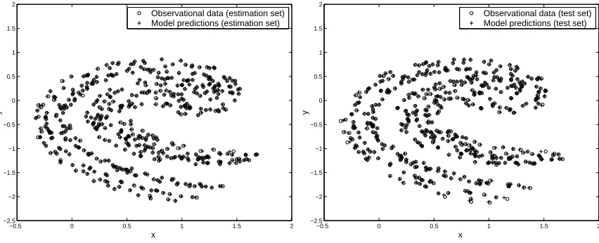
(an arbitrarily small coefficient for D-optimality). The iterative procedure of the proposed algorithm was applied. The model was automatically ter-minated at a, , centers networks. The final basis pursuit
parameter was derived atzP9 6.
A
N+*
. The modelling MSE for the test data set is derived at 6
- ,.A
N+0
. Equiv-alently 6 1
output variance of the test data has been ex-plained by the model. To illustrate the overall performance of the model in capturing the underlying system dynamics, the modelling results for both estimation and test data set is shown in Figure 1.
5. CONCLUSIONS
−0.5 0 0.5 1 1.5 2 −2.5
−2 −1.5 −1 −0.5 0 0.5 1 1.5 2
x
y
Observational data (estimation set) Model predictions (estimation set)
−0.5 0 0.5 1 1.5 2
−2.5 −2 −1.5 −1 −0.5 0 0.5 1 1.5 2
x
y
[image:6.595.87.513.91.264.2]Observational data (test set) Model predictions (test set)
Figure 1: Modelling results for illustrative example.
6. REFERENCES
[1] R. Bellman, Adaptive Control Processes. Princeton University Press, 1966.
[2] C. J. Harris, X. Hong, and Q. Gan, Adaptive
Mod-elling, Estimation and Fusion from Data: A
Neuro-fuzzy Approach. Springer-Verlag, 2002.
[3] M. Brown and C. J. Harris, Neurofuzzy Adaptive
Mod-elling and Control. Prentice Hall, Hemel Hempstead,
1994.
[4] J. S. R. Jang, C. Sun, and E. Mizutani, Neuro-Fuzzy
and Soft Computing: A Computational Approach to
Learning and Machine Intelligence. Upper Saddle
River, NJ : Prentice Hall, 1997.
[5] T. Takagi and M. Sugeno, “Fuzzy identification of systems and its applications to modelling and con-trol,” IEEE Trans. on Systems, Man, and Cybernetics, vol. 15, pp. 116–132, 1985.
[6] S. Chen, S. A. Billings, and W. Luo, “Orthogonal least squares methods and their applications to non-linear system identification,” International Journal of
Con-trol, vol. 50, pp. 1873–1896, 1989.
[7] S. Chen, Y. Wu, and B. L. Luk, “Combined genetic al-gorithm optimization and regularized orthogonal least squares learning for radial basis function networks,”
IEEE Trans. on Neural Networks, vol. 10, pp. 1239–
1243, 1999.
[8] M. J. L. Orr, “Regularisation in the selection of radial basis function centers,” Neural Computation, vol. 7, no. 3, pp. 954–975, 1995.
[9] H. Akaike, “A new look at the statistical model identi-fication,” IEEE Trans. on Automatic Control, vol. AC-19, pp. 716–723, 1974.
[10] A. C. Atkinson and A. N. Donev, Optimum
Experi-mental Designs. Clarendon Press, Oxford, 1992.
[11] X. Hong and C. J. Harris, “Nonlinear model structure design and construction using orthogonal least squares and d-optimality design,” IEEE Transactions on
Neu-ral Networks, vol. 13, no. 5, pp. 1245–1250, 2001.
[12] S. Chen, X. Hong, and C. J. Harris, “Sparse ker-nel regression modelling using combined locally reg-ularised orthogonal least squares and d-optimality ex-perimental design,” IEEE Trans. on Automatic
Con-trol, vol. 48, no. 6, pp. 1029–1036, 2003.
[13] D. J. C. MacKay, “Bayesian methods for adaptive models,” Ph.D. dissertation, California Institute of Technology, USA, 1991.
[14] S. S. Chen, D. L. Donoho, and M. A. Saunders, “Atomic decomposition by basis pursuit,” SIAM
Re-view, vol. 43, no. 1, pp. pp129–159, 2001.
[15] B. Efron, I. Johnstone, T. Hastie, and R. Tibshirani, “Least angle regression,” Annals of Statistics, p. To Appear, 2003.
[16] X. Hong, M. Brown, S. Chen, and C. J. Harris, “Sparse model identification using orthogonal forward regres-sion with basis pursuit and d-optimality,” Submitted to
IEE Proc. - Control Theory and Applications, 2003.