Abstract—Turbulence transition in boundary layer flows arises from nonlinear wave generation, interaction, and amplification in the flow. The nonlinear wave dynamics depend on the intricate phase synchronization of the propagating waves. Numerical simulation of the process encounters challenges in the forms of achieving sufficient computational resolution, dealing with truncated computational domains, and control of numerical errors. Application of high-order, optimized Combined Compact Difference numerical methods help to mitigate these issues and achieve realizations of nonlinear wave dynamics during turbulence transition. Validation of the numerical results attests to the accuracy of the model.
Index Terms—turbulence, transition, combined compact difference, nonlinear wave dynamics
I. INTRODUCTION
he classical work Schubauer and Skramstad, 1947 [1] conducts a famous experiment to examine the topic of boundary layer turbulence transition. The experiment entails a vibrating ribbon that is placed at the base of the inlet to a flow channel and acts to introduces perturbations into the flow. The perturbations convert to disturbance waves that travel downstream. As the disturbance waves propagate downstream, they will begin to interact with one another in progressive stages of transition towards flow turbulence. Initially, the wave interactions are linear in the linear instability stage [2]. Further downstream, the wave interactions will evolve to become linear. The non-linear interactions will spawn a secondary instability in the flow. The secondary instability will eventually become unsustainable and break down into turbulence. The stages of transition up to the linear instability stage are well-understood presently. The linear wave interactions can be described accurately with the Orr-Sommerfeld (OS) equation of linear stability theory. Chen and Chen, 2010 [3] offers an excellent study of the linear stage of turbulence transition. However, once the waves undergo non-linear interactions, the transition phenomenon becomes mysterious and is the subject of much current research.
Manuscript received December 8, 2010; revised January 11, 2011; supported by Ministry of Education Grant RG 4/07.
*JC Chen, Corresponding Author, Nanyang Technological University, School of Civil and Environmental Engineering, Singapore (phone: +65 6790-5273; fax: +65 6790-5273; e-mail: [email protected])
Weijia Chen, Nanyang Technological University, School of Civil and Environmental Engineering, Singapore (e-mail: [email protected])
A subsequent classical work, Klebanoff, et al., 1962 [4] would shed illuminating insight into the non-linear stage of transition. As transition to turbulence can occur via multiple pathways, Klebanoff, et al., 1962 [4] studies the pathway that has come to bear the namesake of its author, K-type transition. When the amplitude of the initial perturbation exceeds 1% of the mean flow, the K-type transition mechanism activates to induce an explosive amplification of waves leading to breakdown into turbulence. Klebanoff, et
al., 1962 [4] observes definitive and reproducible behavior of non-linear wave interactions beginning with the formation of the first set of waves from the perturbation known as the fundamental waves. The fundamental wave exercises a fecundity that begets second and third harmonics of successively higher wave frequencies. The harmonics would then cluster in wave packets as they traverse downstream. Within the packets, the waves interact and synchronize. The phase synchronization of the waves results in explosive spikes in the observed wave oscillations. These observations have become bespoke signature features of non-linear turbulence transition [4].
Additional classical works would ensue. Kachanov and Levchenko, 1984 [5] and Kachanov, 1994 [6] reveal another possible pathway towards turbulence called the N-type transition. The N-N-type transition facilitates a more controlled pathway to turbulence, evoked by a lower amplitude of the initial disturbance than K-type transition. As such, the N-type transition transpires with measurably exponential amplification of waves as contrasted with the incontinent explosion in the K-type. Also, the N-type transition generates harmonics of lower frequencies than the K-type. For more details, Herbert, 1988 [7] offers an excellent review of the physical processes occurring in the non-linear transition stage.
The perspicacity of the aforementioned procession of classical works, though worthy of fete, has only begun to enervate the confounding complexity of the turbulence transition phenomenon. The nature of turbulence transition remains shrouded in mystery to the present time.
II. ISSUES OF CONCERN
The numerical simulation of boundary layer turbulence transition meets with several challenges. The simulation endeavor must successfully contend with these issues of concern so that it can attain accurate and precise realizations of the transition process.
Numerical Realization of Nonlinear Wave
Dynamics in Turbulence Transition Using
Combined Compact Difference Methods
JC Chen* and Weijia Chen
T
A. Computational Resolution
The wave interaction dynamics underlying the transition to turbulence presents a view of the process from the perspective of periodic oscillations of the disturbance velocities in wave form. A concomitant perspective views the process in terms of the formation and deformation of physical flow structures during transition. Some of the commonly observed flow structures include the Λ-vortex,
Ω-vortex, high shear layer, and turbulent streaks [3]. An important physical flow structure of note is the formation of turbulent eddies strewn intermittently throughout the flow. The intermittent turbulent eddies also experience progeneration where first generation eddies beget second and third generations in cascading fashion ([8], [9], and [10]). The posterior eddies will sequentially decrease in length and time scales, imposing taxing demands on the computational power required to visualize them. Chen, 2009 [8] offers an excellent exposition on the eugenics of turbulent eddy progeneration. The numerical simulation must have the computational capacity to reach the necessary level of computational resolution.
Further exacerbating the situation is the concept of three-dimensionality. During the transition towards turbulence, the generated waves will acquire a three-dimensional characteristic. The formation of three-dimensional waves represents a key development in the transition towards turbulence. Saric, et al., 2003 [11] explains that the three-dimensional waves arise from crossflow and centrifugal instabilities occurring in flow regions with pressure gradients. The three-dimensional nature of the flow is the critical element that leads to rapid generation of additional harmonics and their subsequent explosive or exponential amplification. Orszag and Patera, 1983 [12] notes that, during wave interactions, the two-dimensional waves are unstable to the presence of even infinitesimal three-dimensional waves and will amplify exponentially from the encounter. Orszag and Patera, 1983 [12] systematically illustrates that the combination of vortex stretching and tilting terms in the governing Vorticity Transport Equation accelerates the growth of waves. Both vortex stretching and tilting are required to produce the accelerated growth of waves [12]. Both are three-dimensional phenomena and thus, concurringly underline the important role of three-dimensionality in turbulence transition. Reed and Saric, 1989 [13] and Herbert, 1988 [7] offer excellent reviews of the mechanisms that cause the formation of dimensional waves. Numerical visualization of three-dimensional waves incurs vast computational demands.
Even further immiseration in regard to computational demands comes in the form of the critical Reynolds number. The putative work, Orszag and Kells, 1990 [14], explains that, for the transition to turbulence to be sustainable, the flow Reynolds number must exceed a critical threshold value. The fact that a critical Reynolds number exists for turbulence transition has been corroborated by other works of Orszag and Patera, 1983 [12] and Saric, et al., 2003, [11]. Towards the study of non-linear wave interaction dynamics, the critical Reynolds number carries a vexatious implication. The resolution of computational grids needed to realize turbulent flow structures scales exponentially with the Reynolds number (number of grid points ~ ⁄ ) [3].
Hence, for transition to occur, the Reynolds number must surpass a critical threshold, and the numerical visualization of the transition process at that Reynolds number requires a computational grid that scales exponentially with it. The exponential correlation between the Reynolds number and computational grid causes the computational demands to quickly reach impractical levels for even typical turbulent flow conditions.
Clearly then, due to the amalgamation of these issues, microscopic length scales of turbulent eddies, three-dimensionality, and critical Reynolds number, the computational demands weigh onerously on numerical simulations of turbulence transition. Computational capacity of the present time cannot meet such demands for flows of physically realistic dimensions within practical simulation runtime limits. The limitation in computational capacity leads to a follow-up challenge, well-renowned as the Open Boundary Condition (OBC) problem.
B. Open Boundary Condition Problem
Because present-day computational capacity cannot practically realize turbulence transition for flows of realistic physical dimensions, the computational domain must be truncated to maintain satiable computational demands. This truncation creates its own problems. Questions now arise regarding what should be the correct boundary conditions stipulated at the points of truncation. In general, for boundary layer flows, the domain will be truncated at the freestream and outflow boundaries. For the freestream boundary, because it lies transverse to the prevailing flow, the disturbance vorticity will decay rapidly along that direction, making the boundary conditions there relatively manageable. However, the case of the outflow boundary stands as a formidable challenge, because it lies in-line with the flow direction and the downstream direction of the amplifying waves. The propagating waves will exit the domain at the outflow boundary while potentially still containing appreciable wave amplitudes. How to correctly define the outflow boundary conditions becomes a topic of much longstanding controversy and debate. The outflow boundary conditions must be defined in such a way as to prevent the exiting waves from reflecting back into the domain to cause numerical errors. This issue is known as the Open Boundary Condition (OBC) problem.
solutions for non-reflecting OBC’s include Jin and Braza, 1993 [16], Hedstrom 1979 [17], Rudy and Strikwerda, 1980[18], and Johansson, 1993 [19]. Another excellent review of OBC’s is given in Gresho, 1991 [20].
Since the correct definition of the OBC proves to be querulous, perhaps then, it would be expedient to eschew the topic by appealing to the convenience of using a buffer domain. A buffer domain implements a damping function near the outflow that would dissipate the waves prior to their exit. Other works that practice this strategy include Streett, 1989 [21] and Meitz, et al., 2000 [22].
The insertion of an artificial buffer domain onto an artificial truncation of that domain merely trades one problem for another. Unsurprisingly, a new problem emerges, this time in the form of grid-mesh oscillations. The buffer domain inserts a discontinuity into the flow domain that will generate oscillating numerical errors of high wave numbers that can flow back upstream to distort the true wave dynamics. Furthermore, the buffer domain forcibly damps waves that potentially could still be amplifying. The coerced damping against the amplifying will of the waves results in violent oscillations with clearly visible shaking of the wave motion, as the waves struggle against the suppression of the buffer domain. Grid-mesh oscillations declare a very important issue of contention in the simulations of turbulence: control of numerical errors.
C. Numerical Errors
Nonlinear wave generation, interaction, and amplification in boundary layer turbulence transition rely heavily on the intricate minutiae underlying synchronization of the phases and amplitudes of the propagating wave packets. As such, the presence of pernicious numerical errors exacts a noisome toll on the accuracy and precision of the numerical visualizations with potentially disastrous consequences. One of the sources of numerical errors emanates from the buffer domain. The buffer domain prevents the exiting waves from reflecting back upstream but at the cost of introducing its own errors in the form of grid-mesh oscillations. Other types of errors can be introduced from the numerical discretization of the governing equations of the flow. With finite difference discretizations, numerical dissipiation, dispersion, and aliasing errors become relevant.
Dissipation errors pertain to the accurate depiction of the amplitudes of the propagating waves. The flow contains natural viscous dissipative forces. So, dissipation errors can emerge simply from inaccurate accounting for the effects of viscous dissipation ([2], [23], and [24]). In addition, the numerical discretization can generate pseudo-dissipative mechanisms in the simulation that otherwise should not be present at all ([2], [23], and [24]). These would be numerical dissipation errors. Dissipation errors impact the amplification behavior within the wave interaction dynamics, and wave amplification is a key component of the turbulence transition process.
Dispersion errors deal with the phase velocities of the traveling waves, as well as, the relative velocities amongst waves within a group or packet. The effects of dispersion errors cause the wave velocities to drift away from their true speeds ([2], [23], and [24]). This can lead to incorrect lagging or acceleration of the traveling waves, or even
worse, a false total reversal in the direction of propagation. Dispersion errors affect the phase synchronization of the interacting waves, and this synchronization is the flywheel that drives wave generation, interaction, and amplification in boundary layer turbulence transition.
Perhaps, the most dyspeptic prospects egress from aliasing errors. The interactions of the propagating waves produce additional waves with increasing wave numbers. For simulations with insufficient numerical resolution, the high wave number waves would need to be interpolated or aliased onto the grid as lower wave number waves. The incorrect representation of the high wave number wave as a lower wave number wave will cause numerical instabilities that culminate in the apprehensive scenario of numerical blow-up ([25] and [26]). Indeed, aliasing error threatens potential disaster if the numerical simulation does not adequately address its catastrophic influence.
So then, the discussion heretofore should elucidate the both the detracting and devastating aspects of numerical errors. Therefore, the abeyance of numerical errors poses a mandate of utmost importance. Combined compact difference numerical methods offer a viable tool for surmounting the preceding jeremiad in regards to the challenges confronting the numerical simulations of wave dynamics occurring in boundary layer turbulence transition.
III. PROBLEM DEFINITION
The governing equations for turbulence transition in boundary layer flow are the Navier-Stokes (NS) equations. For better ease of defining the flow conditions at the boundaries, the NS equations undergo a conversion to its variant form, the Vorticity Transport Equation (VTE). Chen and Chen, 2010 [3] provides copious discussions on the transformation procedure and its mathematical implications. The total set of governing equations for two-dimensional flows comprise the VTE given in (1), the Velocity-Poisson’s Equation in (2), and the continuity condition in (3):
2 2 2 2
1
y
Ω
x
Ω
Re y
Ω
V x
Ω
U t
Ω
∂ ∂ + ∂ ∂ = ∂ ∂ + ∂ ∂ + ∂
∂ (1)
x
Ω
y V x
V
Re ∂
∂ − = ∂ ∂ + ∂ ∂
2 2 2 2
1 (2)
y x
V x
U
∂ ∂
∂ − = ∂
∂ 2
2 2
(3) where Uis the velocity in the x-direction, V is the velocity
in the y-direction, and Ω is the vorticity. The numerical model can be extended to three-dimensional flows once the accuracy of the two-dimensional model has been established. The flow parameters U, V, and Ω consist of steady, time-independent base flow components, UB, VB, and ΩB, with no disturbances and time-dependent components, u, v, and ω, that account for the disturbance:
) , , ( ) , ( ) , ,
(x y t U x y u x yt
U = B + (4)
) , , ( ) , ( ) , ,
(x yt V x y v x y t
V = B + (5)
). , , ( ) , ( ) , ,
(x yt Ω x y x yt
Ω = B +ω (6)
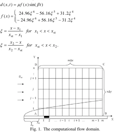
Figure 1 shows the flow domain. Truncations to the domain occur at the freestream boundary CD and outflow boundary BC. The perturbation is introduced into the flow at the location of the black block in the form of a blowing
and suction strip modeled by a sinusoidal function: ) sin( ) ( ) ,
(xt f x t
d =μ β (7)
⎪⎩ ⎪ ⎨ ⎧ − + − + −
= 66 55 44
2 . 31 16 . 56 96 . 24 2 . 31 16 . 56 96 . 24 ) ( ξ ξ ξ ξ ξ ξ x
f (8)
st 1 1 st
1 for x x x
x x
x
x < <
− − =
ξ (9)
.
2 st st 2
2 for x x x
x x
x
x < <
− − =
[image:4.612.71.270.58.289.2]ξ (10)
Fig. 1. The computational flow domain.
Chen and Chen, 2010 [24] expounds on the boundary conditions. Noteworthy are the freestream and outflow boundaries. The freestream boundary conditions are:
v Re y
v=− α
∂
∂ (11)
0 2 2 = ∂ ∂ = ∂ ∂ = y y ω ω
ω (12)
where α is the linear disturbance wave number.
The OBC problem at the outflow boundary is treated by a buffer domain. The buffer domain damps ω between a designated point x = xB and the outflow boundary by
multiplying ω to a damping function T(Lb) given in Fig. 2:
. M B
B
b x x
x x L
− −
[image:4.612.71.283.425.568.2]= (13)
Fig. 2. The damping function.
After damping, the outflow boundary conditions are: . 0 2 2 2 2 2 2 = ∂ ∂ = ∂ ∂ = ∂ ∂ x x v x
u ω (14)
The insertion of the buffer domain interjects a discontinuity that produces grid-mesh oscillating errors with high wave numbers. To preserve the accuracy and precision of the numerical simulation, the grid-mesh oscillations must be suppressed along with other types of numerical errors, dissipation, dispersion, and aliasing errors.
IV. NUMERICAL METHOD
A. Combined Compact Difference Schemes
High-order combined compact difference (CCD) schemes
provide the dual advantages of accuracy of simulations and control of numerical errors. The CCD scheme combines the discretization for the function, f, its first derivative, F, and second derivative, S, with a, b, and c as the coefficients of the numerical scheme and h as the grid size:
0 2 1 2 1 2 1 , 1 , 1 2 ,
1 +
∑
+∑
=∑
= + = + = + j j j j j j j j j j i j j j j j ijF h b S c f
a
h (15)
. 0 2 1 2 1 2 1 , 2 , 2 2 ,
2 +
∑
+∑
=∑
= + = + = + j j j j i j j j j j i k j j j j ijF h b S c f
a
h (16)
A 5-point CCD scheme involves points at i = -2, -1, 0, 1, 2. To derive a CCD scheme of 12th-order accuracy, there will be 15 coefficients each for (15) and (16). The parameters bp,2 (p = 1, 2) should be set as 1 for
normalization. Then, bp,0 and bp,1 are free for selection. The
other 12 parameters are obtained from matching the Taylor series up to 12th-order.
The discretizations of the spatial derivative terms involving 2
2 x ∂ ∂ , y ∂ ∂
, and 2 2
y ∂
∂
in (1) to (3) use 12th-Order Centered-Difference Combined Compact Difference schemes hereafter referred to as CCCD12. The high order of the numerical discretizations here will suppress dissipation and dispersion errors. The discretization of the downstream convective term
x Ω U
∂ ∂
uses a 12th-Order Upwind-type Combined Compact Difference scheme hereafter referred to as UCCD12. The upwind nature of this discretization scheme will suppress the grid-mesh oscillations arising from the buffer domain. The discretization of the temporal derivative in (1) uses a 4th -order 5-6 alternating stages Runge-Kutta (RK) scheme based on Hu, et al., 1996 [27].
B. Control of Numerical Errors
The effectiveness of the CCCD12 and UCCD12 schemes in controlling numerical errors can be examined using Modified Wave Number analysis. This method takes the Fourier transform of (15) and (16) to consider the numerical errors in spectral space:
( ) ( )
( ) 0
exp exp exp 2 2 , 1 2 2 , 1 2 2 2 2 , 1 1 = + +
∑
∑
∑
− = − = − = i j i j i j Iiw c f Iiw b f w Iiw a f Iw ) ) ) (17) ( ) ( )( ) 0
exp exp exp 2 2 , 2 2 2 , 2 2 2 2 2 , 2 1 = + +
∑
∑
∑
− = − = − = i j i j i j Iiw c f Iiw b f w Iiw a f Iw ) ) ) (18)where is the Fourier transform of f, , and is the scaled wave number, the wave number multiplied by the grid size Δx. Due to numerical errors, the scaled wave numbers will be modified. The parameters w1 andw2are the
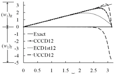
modified scaled wave numbers for the discretizations of the first and second derivatives, respectively. The modified scale wave numbers are complex numbers, whereas the true scale wave numbers are purely real numbers. Figure 3 shows a comparison between the modified and true scaled wave numbers for the first derivative discretizations using the CCCD12, UCCD12, and ECD1st12 (12th-Order Explicit
x k w= Δ
Centered-Difference) schemes. The subscripts R and I represent the real and imaginary parts, respectively. Deviations of the real part of the modified scale wave number from the true value w will cause dispersion errors. Deviations of the imaginary part, which should be zero since
[image:5.612.317.543.154.322.2]w is a real number, will give rise to dissipation errors. Figure 3 indicates that, the real parts of the modified scale wave number, (w1)R, for the CCCD12 and UCCD12
schemes remain close to the true value w for a longer range than the ECD1st12 scheme. So, the two former schemes should display greater accuracy and lower dispersion errors than the latter. The UCCD12 scheme is the only method that exhibits an imaginary part, increasing rapidly at high scaled wave numbers to signify powerful dissipation.
Fig. 3. Comparison between the modified and true scaled wave numbers for the first derivative discretization.
The numerical method can be optimized to leverage upon the high accuracies of CCCD12 and UCCD12 schemes and the dissipative tendencies of the UCCD12 scheme at high wave numbers. The idea here is to choose the grid size Δx and coefficients of the UCCD12 and 5-6 RK schemes such that the physical waves for simulation will fall in the range where (w1)Rremains close to w for accurate realizations.
Then, the grid-mesh oscillating errors with high wave numbers will be made to enter into the high dissipation range and be dissipated by the imaginary part (w1)I.
V. RESULTS AND DISCUSSIONS
[image:5.612.96.281.220.339.2]To establish confidence in the accuracy of the numerical model, its simulations of linear instability can be validated versus the OS equation. Figure 4 shows a comparison between model predictions and solutions of the OS equation for the wall-normal profiles of flow parameters u, v, and ω. The results of the model and the OS equation completely overlap, averring excellent agreement.
Fig. 4. Validation of the numerical model versus linear stability theory and the OS equation. Initial disturbance A0 = 0.009% of the freestream velocity to maintain linear waves. Downstream x-locationRex= xRe=400.
With confidence assured, the matter at hand shifts to the investigation of nonlinear wave generation, interaction, and amplification in boundary layer turbulence transition. Figure 5 delivers a numerical realization to this effect. The numerical visualization of the downstream evolution of the
u-disturbance velocity vividly describes the sequence where disturbance waves manifest then amplify in their amplitudes as they traverse downstream. Indeed, the targeted nonlinear wave dynamics have been realized.
Fig. 5. Downstream amplification behavior of the u-disturbance velocity. Amplitude of initial disturbance A0 = 0.3% of the freestream velocity.
Notice a critical development occurring at the buffer domain. When the waves arrive at the buffer domain, their amplification persists. However, the damping function of the buffer domain forcibly compels the amplifying waves to damp. The struggle between the natural amplifying tendencies of the waves and the forced damping of the buffer domain produces a visible shaking of the waves in the simulation. Numerical errors caused by the disruption from the buffer domain are quite obvious, as is the importance of controlling these errors. The oscillations at the buffer domain tend to have high wave numbers, and the numerical method can eliminate them using the dissipative mechanisms of the UCCD12 scheme shown in Fig. 3.
Figure 6 shows Fourier decomposition of the flow field in Fig. 5 and depicts four constituent wave components 1F to 4F. The 4F wave has four times the frequency as the 1F. Notice here that the 3F and 4F waves display amplitudes orders of magnitude lower than the 1F and 2F. The microscopic amplitudes of the 3F and 4F waves render them especially vulnerable to distortions from numerical dissipation, dispersion, and aliasing errors. The high-order CCCD12 schemes applied to the spatial derivatives control the numerical errors and preserve the low-amplitude waves. Notice further that the 4F wave has a scaled wave number of 2.25, which according to Fig. 3, places it safely in the region before the large dissipative effects at high wave numbers. So, the delicate 4F wave can be protected from this risk.
An immediate riposte that inveighs upon this result should be addressed, and that is, the dissipative mechanism of the UCCD12 scheme can destroy high wave number physical waves that may be crucial to the wave interaction dynamics. In fact, the dominance of microscopic-scale eddies in turbulence suggests that high wave number physical waves would seem especially relevant to the
[image:5.612.76.298.603.696.2]process. The remedy to this conundrum would call for rigorous further study of the wave interaction dynamics to astutely demarcate the cut-off point for realizing high wave number waves. Beyond the cut-off point, the waves can be allowed to be dissipated. In Fig. 6, the justification for realizing up to the 4F wave contends that inclusion of higher wave number waves would not produce appreciable changes to the overall disturbance amplification.
Fig. 6. Fourier transformation of the fully developed flow field given in Fig. 5 at the wall-normal location y = 0.7.
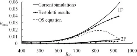
Figure 7 exhibits qualitative agreement between the model predictions and the work of Bertolotti, et al., 1992 [28] for the amplification behaviors of the 1F and 2F waves. Also, the 1F wave amplifies faster than the prediction from the OS equation due to the inclusion of nonlinear interaction effects. These results attest to the accuracy of the model.
Fig. 7. Comparisons of simulation results of nonlinear amplification of the maximum disturbance velocity umax with linear stability theory and Bertolotti, et al., 1992 [28].
VI. CONCLUSION
This has been an illuminating discourse on non-linear wave generation, interaction, amplification in boundary layer turbulence transition. This fascinating problem traces from the classical works of Schubauer and Skramstad, 1947 [1], Klebanoff, et al., 1962 [4], and Kachanov and Levchenko, 1984 [5]. Important challenges confront the numerical simulation of turbulence transition in terms of considerations for computational resolution, the OBC problem, and control of numerical errors. The numerical model uses high-order, optimized CCD schemes to preserve the physical waves, while dissipating numerical errors with high wave numbers. Numerical realizations resplendently demonstrate the wave dynamics and its underlying constituent components. Validation of the model versus linear stability theory and other works of non-linear wave dynamics asserts confidence and legitimacy. The numerical model can be extended to three-dimensions to realize the full turbulence transition process and to address the issue of meeting the requisite computational demands.
REFERENCES
[1] G. Schubauer and H. K. Skramstad, “Laminar boundary layer oscillations and stability of laminar flow,” J. Aeronaut. Sci., vol. 14, no. 2, pp. 69-78, 1947.
[2] J. Chen and W. Chen, “Turbulence transition in two-dimensional boundary layer flow: Linear instability,” in Proc. 6th Intl. Conf. Flow
Dyn., Sendai, Japan, 2009, pp. 148-149.
[3] J. Chen and W. Chen, “The complex nature of turbulence transition in boundary layer flow over a flat surface,” Intl. J. Emerg. Multidiscip. Fluid Sci., vol. 2, no. 2-3, pp. 183-203, 2010.
[4] P. S. Klebanoff, K. D. Tidstrom and L. M. Sargent, “The three-dimensional nature of boundary-layer instability,” J. Fluid Mech., vol. 12, no. 1, pp. 1-34 1962.
[5] Y. S. Kachanov and V. Y. Levchenko, “The resonant interaction of disturbances at laminar-turbulent transition in a boundary layer,” J. Fluid Mech., vol. 138, pp. 209-247, 1984.
[6] Y. S. Kachanov, “Physical mechanisms of laminar-boundary-layer transition,” Annu. Rev. Fluid Mech., vol. 26, pp. 411-482 1994. [7] T. Herbert, “Secondary instability of boundary layers,” Annu. Rev.
Fluid Mech., vol. 20, pp. 487-526, 1988.
[8] J. Chen, “The law of multi-scale turbulence,” Intl. J. Emerg. Multidiscip. Fluid Sci., vol. 1, no. 3, pp. 165-179, 2009.
[9] G. K. Batchelor, The theory of homogeneous turbulence. Student's edition. London: Cambridge University Press, 1953.
[10] A. S. Monin and A. M. Yaglom, Statistical fluid mechanics: Mechanics of turbulence II. Mineola: Dover Publications, 1975. [11] W. S. Saric, H. L. Reed and E. B. White, “Stability and transition of
three-dimensional boundary layers,” Annu. Rev. Fluid Mech., vol. 35, pp. 413-440, 2003.
[12] S. A. Orszag and A. T. Patera, “Secondary instability of wall-bounded shear flows,” J. Fluid Mech., vol. 128, pp. 347-385, 1983.
[13] H. L. Reed and W. S. Saric, “Stability of three-dimensional boundary layers,” Annu. Rev. Fluid Mech., vol. 21, pp. 235-284, 1989. [14] S. A. Orszag and L. C. Kells, “Transition to turbulence in plane
Poiseuille and plane Couette flow,” J. Fluid Mech., vol. 96, no. 1, pp. 159-205, 1980.
[15] R. L. Sani and P. M. Gresho, “Resume and remarks on the open boundary condition minisymposium,” Intl. J. Numer. Methods Fluids, vol. 18, no. 10, pp. 983-1008, 1994.
[16] G. Jin and M. Braza, “A non-reflecting outlet boundary condition for incompressible unsteady Navier-Stokes calculations,” J. Comput. Phys., vol. 107, no. 2, pp. 239-253, 1993.
[17] G. W. Hedstrom, “Nonreflecting boundary conditions for nonlinear hyperbolic systems,” J. Comput. Phys., vol. 30, pp. 222-237, 1979. [18] D. H. Rudy and J. C. Strikwerda, “A nonreflecting outflow boundary
condition for subsonic Navier-Stokes calculations,” J. Comput. Phys., vol. 36, no. 1, pp. 55-70, 1980.
[19] B. Christer and V. Johannson, “Boundary conditions for open boundaries for the incompressible Navier-Stokes equation,” J.
Comput. Phys., vol. 105, pp. 233-251, 1993.
[20] P. M. Gresho, “Incompressible fluid dynamics: Some fundamental formulation issues,” Annu. Rev. Fluid Mech., vol. 23, pp. 413-453, 1991.
[21] C. L. Streett and M. G. Macaraeg, “Spectral multi-domain for large-scale fluid dynamic simulations,” Appl. Numer. Math., vol. 6, no. 1-2, pp. 123-139, 1989.
[22] H. L. Meitz and H. F. Fasel, “A compact-difference scheme for the Navier-Stokes equations in vorticity-velocity formulation,” J.
Comput. Phys., vol. 157, no. 1, pp. 371-403, 2000.
[23] J. Chen and W. Chen, “Combined compact difference method for simulation of nonlinear wave generation, interaction, and amplification in boundary layer turbulence transition,” in Proc.7th
Intl. Conf. Flow Dyn., Sendai, Japan, 2010, pp. 82-83.
[24] W. Chen and J. Chen, “Direct numerical solution of Navier-Stokes equations by combined compact difference methods for simulations of boundary layer turbulence transition,” Intl. J. Numer. Methods Fluids, submitted for publication.
[25] P. Moin and K. Mahesh, “Direct numerical simulation: A tool in turbulence research,” Annu. Rev. Fluid Mech., vol. 30, pp. 539-578, 1998.
[26] S. L. Lyons and T. J. Hanratty, “Large-scale computer simulation of fully developed turbulent channel flow with heat transfer,” Intl. J. Numer. Methods Fluids, vol. 13, no. 8, pp. 999-1028, 1991.
[27] F. Q. Hu, M. Y. Hussaini and J. L. Manthey, “Low-dissipation and low-dispersion Runge-Kutta schemes for computational acoustics,” J. Comput. Phys., vol. 124, no. 1, pp. 177-191, 1996.
[image:6.612.74.304.383.477.2]