Online Full Text

Abstract—Sub-harmonic resonance in zero pressure

gradient three-dimensional boundary layer flow occurs in the classical N-type pathway of turbulence transition. Three-dimensionality incurs exorbitant computational demands on the numerical simulations. Imposition of a spectral method and a non-uniform grid countervails the impractical computational demands. Eigenvalue analysis ascertains ranges of stability of the numerical method. Validation of the numerical method versus the three-dimensional OS equation avers confidence in the accuracy of the model. Numerical realizations of the generation, amplification, and interaction of two- and three-dimensional sub-harmonic waves agree qualitatively with classical experiments.

Index Terms— sub-harmonic resonance, spectral method,

non-uniform grid, three-dimensional boundary layer flow

I. INTRODUCTION

ow does flow become turbulent? The profundity of the question mandates a meticulous deconstruction of its coadjuvantly interacting metaphysics. Underneath the artifice of seemingly chaotic cacophony lie deterministic symphonies of motion. To the present day, knowledge of turbulence transition remains inchoate. Some bespoke phenomena have consistently manifested in both experimental visualizations and numerical simulations. At the onset of turbulence transition, the flow becomes three-dimensional, characterized by spanwise modulations of the streamwise velocity and the formation of a mysterious flow structure known as the Soliton-like Coherent Structure (SCS) [1-4]. An SCS is a strong, concentrated, self-enforcing non-linear wave. It can persist for long durations of time, and it is strong in that it emerges from interactions with other SCSs with little change to its structures except for a shift in phase [3, 5, 6]. The SCSs travel downstream at much slower speeds than the mean boundary layer flow. However, the transverse flow velocity in the SCS is close to the mean flow velocity [6]. So, the SCS will tend to shed a secondary closed vortex in the upward direction. The interactions among the SCSs will ultimately lead to them merging together to form elongated low-speed streaks of coherent structures along the wall of the boundary layer [6].

The SCSs and the spanwise modulation of velocity induce the formation of a signature structure of turbulence transition, the Λ-vortex [7, 8]. The Λ-vortices form at the

Manuscript received 9 April, 2012. Supported by Ministry of Education Grant RG 4/07.

*JC Chen, Corresponding Author, Nanyang Technological University, School of Civil and Environmental Engineering, Singapore (phone: +65 6790-5273; fax: +65 6790-5273; e-mail: [email protected])

Chen Weijia, Nanyang Technological University, School of Civil and Environmental Engineering, Singapore

peak locations of the spanwise modulation [1, 3, 5]. The legs of the Λ-vortex comprise two tubes of streamwise vortices [9-12]. Above the Λ-vortex, a high shear layer develops featuring rapidly increasing velocity gradients [1, 8-11, 13-15]. The interaction between the Λ-vortex and the high shear layer leads to a peculiar phenomenon. The Λ -vortex will incline and lift upwards [4, 5, 11, 15, 16]. The inclination of the Λ-vortex causes its tip to enter into the region of high shear. The high shear stretches the tip of the Λ-vortex and elongates it [5, 11]. The elongating tip deforms into an Ω-shaped vortex [1, 5]. Further elongation would lead to the Ω-vortex detaching from the Λ-vortex. The detached ends of the Ω-vortex would reconnect to close the loop to form a ringed vortex [5].

At this point, the ringed vortex travels downstream and becomes a most crucial element of turbulence transition, the turbulent spot [8, 17, 18]. The turbulent spot is believed to be the flashpoint from which transition to turbulence initiates. Consecutive ringed vortices would overtake one another downstream, propelled by the high shear layer, and merge [8]. Within the ringed vortex, disturbance waves generated in the flow propagate in concert in the form of wave packets. Inside the wave packets the disturbance waves interact and synchronize [3, 18]. This concept is known as space-time focusing of wave energy, made famous by Landahl, 1972 [19]. When the waves synchronize, their mutual additive summation produces spiking signals in the flow velocity, one of the fascinating aspects of turbulence transition [1, 3, 5]. The pulsating spikes resonate to the point of unsustainable breakdown, and hence the onset of flow randomization that leads to turbulence.

The high shear layer would form a “kink” at its apex that then rolls up into a vortex [1, 7, 9]. The rolled-up vortex exhibits similar behavior to that of the ringed vortex with spikes occurring within its core [5]. In fact, the rolled-up vortex has been observed to be in synchronization with the ringed vortex [5]. The rolling up of the high shear layer causes fluid away from the wall to be swept downwards towards the wall and vice versa with eruption of near-wall fluid upwards [9]. The transference of fluid leads to another signature feature of turbulence transition, low-speed streaks of high shear stress moving downstream along the wall famously known as Klebanoff modes [9, 13, 17, 18, 20]. The high shear layer and low-speed streak both will undergo their own instabilities that conclude in breakdown to turbulence [13]. The physical mechanisms and dynamics responsible for the series of phenomena leading to turbulence remains a classical mystery of science. This topic has drawn intense study with an illustrious history.

In the alternative perspective, the classical work, Schubauer and Skramstad, 1947 [21], conducts a famous experiment to examine the topic of boundary layer

How Flow Becomes Turbulent

JC Chen* and Chen Weijia

H

IAENG International Journal of Applied Mathematics, 42:2, IJAM_42_2_05

turbulence transition. The experiment entails a vibrating ribbon that is placed at the base of the inlet to a flow channel and acts to introduce perturbations into the flow. The perturbations evolve into disturbance waves known as Tollmien–Schillichting (TS) waves that travel downstream. As the disturbance waves propagate downstream, they will begin to interact with one another in progressive stages of transition towards flow turbulence. Initially, the wave interactions are linear in the linear instability stage [22]. Further downstream, the wave interactions become nonlinear. The nonlinear interactions spawn a secondary instability in the flow. The secondary instability eventually becomes unsustainable and break down into turbulence. The stages of transition up to linear instability are well-understood presently. The linear wave interactions can be described accurately with the Orr-Sommerfeld (OS) equation of linear stability theory. Chen and Chen, 2010 [23] offers a scholastic study of the linear stage of turbulence transition. However, once the waves undergo nonlinear interactions, the transition phenomenon becomes mysterious and is the subject of much cerebation.

A subsequent classical work, Klebanoff, et al., 1962 [24], would shed illuminating insight into the nonlinear stage of transition. As transition to turbulence can occur via multiple pathways, Klebanoff, et al., 1962 [24] studies the pathway that has come to bear the namesake of its author, K-type transition. When the amplitude of the initial perturbation exceeds 1% of the mean flow, the K-type transition mechanism activates to induce an explosive amplification of waves leading to breakdown into turbulence. Klebanoff, et al., 1962 [24] observes definitive and reproducible behavior of nonlinear wave interactions beginning with the formation of the first set of waves from the perturbation known as the fundamental waves. The fundamental wave exercises a fecundity that begets second and third harmonics of successively higher wave frequencies. The harmonics would then cluster in wave packets as they traverse downstream. Within the packets, the waves interact and synchronize. The phase synchronization of the waves results in explosive spikes in the observed wave oscillations. These observations have become bespoke signature features of nonlinear turbulence transition [24].

Additional classical works would ensue. Kachanov and Levchenko, 1984 [25] and Kachanov, 1994 [3] reveal another possible pathway towards turbulence called the N-type transition. The N-N-type transition facilitates a more controlled pathway to turbulence, evoked by a lower amplitude of the initial disturbance than K-type transition. As such, the N-type transition transpires with measurably exponential amplification of waves as contrasted with the incontinent explosion in the K-type. Also, the N-type transition generates harmonics of lower frequencies than the K-type. The N-type wave interactions are termed sub-harmonic resonance that involves the initial TS disturbance waves of a given frequency and subsequently generated sub-harmonic waves with frequencies / /2. For more details, Herbert, 1988 [4] offers an excellent review of the nonlinear transition stage.

Chen, 2009 [26], Chen and Chen, 2010 [23] Chen and Chen, 2012 [27], Chen and Chen, 2011 [28], Chen and Chen, 2012 [29], Chen and Chen, 2012 [30], Chen and

Chen, 2009 [22], Chen and Chen, 2010 [31], Chen and Chen, 2011 [32], Chen and Chen, 2011 [33], and Chen and Chen, 2012 [34] respectfully anthologize his study of boundary layer turbulence transition.

II. THREE DIMENSIONALITY

During the transition towards turbulence, the generated waves acquire a three-dimensional characteristic. The formation of three-dimensional waves represents a key development in turbulence transition. Saric, et al., 2003 [35] explains that the three-dimensional waves arise from crossflow and centrifugal instabilities occurring in flow regions with pressure gradients. The three-dimensional nature of the flow is the critical element that leads to rapid generation of additional harmonics and their subsequent explosive or exponential amplification. Orszag and Patera, 1983 [36] notes that, during wave interactions, the two-dimensional waves are unstable to the presence of even infinitesimal three-dimensional waves and will amplify exponentially from the encounter. Orszag and Patera, 1983 [36] systematically illustrates that the combination of vortex stretching and tilting terms in the governing Vorticity Transport Equation accelerates the growth of waves. Both vortex stretching and tilting are required to produce the accelerated growth of waves [36]. Both are three-dimensional phenomena and thus, concurringly underline the important role of three-dimensionality in turbulence transition. Reed and Saric, 1989 [12] and Herbert, 1988 [4] offer excellent reviews of the mechanisms that cause the formation of three-dimensional waves.

Study of three-dimensional flows carves a frontier of great interest in cutting-edge fluid dynamics research. However, numerical visualization of three-dimensional waves incurs vast computational demands. The computational demands quickly reach impractical levels for even typical flows. Therefore, easing computational demands to within practical limits poses a mandate of utmost importance. Spectral methods offer such a reprieve.

III. PROBLEM DEFINITION A. Flow Domain

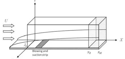
Figure 1 depicts the flow problem as the classical three-dimensional boundary layer flow problem of Schubauer and Skramstadt, 1947 [21]. A blowing and suction strip generates the disturbances. The spanwise z-direction covers one disturbance wavelength . A buffer domain before the outflow boundary ramps down the disturbances to prevent reflection [27, 31].

Fig. 1. Schematic of the flow domain.

IAENG International Journal of Applied Mathematics, 42:2, IJAM_42_2_05

B. Governing Equations

Non-dimensional variables are used. They are related to their dimensional counterparts, denoted by bars, as follows:

, , √ , (1a)

, , √ , and (1b) where the characteristic length 0.05 m, freestream

velocity = 30 m/s, kinematic viscosity = 1.5 × 10-5 m2_{/s, is the Reynolds number, , , and are the} streamwise, transverse, and spanwise flow velocities.

The total flow velocity and vorticity , comprise a steady two-dimensional base flow , and an unsteady three-dimensional disturbance flow , [11, 37]:

, , , , , , , , , (2)

, , , , , , , , , (3)

, , 0 , 0, 0, , and (4)

, , , , , . (5)

The governing equations for the disturbance flow are the Vorticity Transport Equations [11, 37]:

, (6)

, (7)

, (8)

, (9)

, (10)

, and (11)

, , . (12)

In addition, there is a set of Poisson’s equations [11, 37]:

, (13)

, and (14)

. (15)

Finally, the continuity equation completes the set:

0. (16)

Zero pressure gradient (ZPG) boundary layer flow serves as the base flow. The solution procedure begins by solving

the two-dimensional steady base flow followed by the three-dimensional disturbance flow. Chen and Chen, 2012 [27] copiously details this solution algorithm.

C. Boundary Conditions Inflow Boundary Condition

The inflow boundary introduces no disturbances; hence, , , , , , and along with their first and second derivatives are all zero there.

Freestream Boundary Condition

Assuming potential flow at the freestream boundary, the vorticity is zero there:

0, 0, 0, (17)

0, 0, 0, (18)

0, 0, 0, and (19)

√ . (20)

The parameter decays much slower, and so its wall-normal derivative remains appreciable with a prescribed wave number of . The other parameters and would result from the solution of the governing equations.

Wall Boundary Condition

The boundary conditions at the wall are:

0, (21)

0, 0, (22)

0, (23)

, (24)

0, and (25)

. (26)

Correct definition of the wall boundary conditions remains a hotly contested matter. Problematic issues include the need to preserve continuity and vorticity. Chen and Chen, 2010 [23] engages in a tendentious intellection of the issue of defining the wall boundary condition.

The blowing and suction strip shown in Fig. 1 generates disturbances in spectral space according to:

√ sin , (27)

24.96 56.16 31.2

24.96 56.16 31.2 , (28) for the first case, and (29)

IAENG International Journal of Applied Mathematics, 42:2, IJAM_42_2_05

for the second case (30) where = 0 or 1, the disturbance amplitude = 1.0 × 10-4_{, and the disturbance frequency = 10.0. The Fourier} modes = 0 and 1 correspond to the two- and three-dimensional disturbances, respectively.

Outflow Boundary Condition

A buffer domain located at x = xB prior to the outflow

boundary at x = xM ramps down the flow disturbances with

ramping function:

. . . .

. . (31)

. (32) Spanwise Boundary Condition

The spanwise boundaries located at = 0 and = implement periodic boundary conditions where all disturbance flow parameters and their derivatives at = 0 are equal to their counterparts at = .

IV. SPECTRAL METHOD

Spectral methods offer the advantages of exponential convergence, numerical accuracy, and computational efficiency. They have demonstrated superior performance to finite difference methods [38]. Spectral methods approximate the solution to a given set of governing equations, for example, by assuming the solution to be a Fourier series or Chebyshev polynomials [38]. In contrast, finite difference methods approximate the original governing equations and then seek to solve the approximate problem. Spectral methods are especially suited for problems with periodic boundary conditions, which in this study occurs at the spanwise boundaries. This study uses a Fourier series approximation for the solution [11, 37, 39]:

, , , ∑ , , exp (33) where is a flow variable of interest such as the velocity,

, , are the Fourier amplitudes, spanwise wave number 2 ⁄ , and is the largest spanwise wavelength of flow disturbances. The mode is the complex conjugate of , so the governing equations and boundary conditions can be transformed to +1 equations and boundary conditions in the two-dimensional x-y plane.

For cases with symmetric flow, the Fourier expansion can be compacted to sines and cosines separately as [11, 37, 39]:

, , , , ∑ , , , , cos (34)

, , , ∑ , , , sin . (35)

The parameters , , , , and are symmetric; , , , and are anti-symmetric. This compaction requires the simulation of half of the wavelength, /2, hence, reduces computational demands by half [11, 37, 39].

The governing equations in spectral representation are:

, (36)

, (37)

, (38)

, (39)

, and (40)

. (41)

V. OVERALL NUMERICAL METHOD

The present study uses a spectral Fourier method in the spanwise direction. By that, imagine the flow domain shown in Fig. 1 to be divided into a series of x-y planes. For each x-y plane, the governing equations are given according to Eqs. (36) to (41). Each x-y plane would then need its numerical discretization. The spatial discretization uses 12th_{-order Combined Compact Difference (CCD) schemes.} The temporal discretization uses a 4th_{-order 5-6 alternating} stages Runge-Kutta (RK) scheme. Chen and Chen, 2011 [28], Chen and Chen, 2012 [27], and Chen and Chen, 2012 [30] comprise a graphomanic series on the development of these numerical methods.

VI. NON-UNIFORM GRID A. Computational Efficiency

Since the numerical realization of turbulence transition exerts impractically onerous computational demands, one would do well to preserve computational resources as much as possible. One method of conservation uses non-uniform grids that concentrate the computational resolution in regions of interest and relax to coarse resolutions in regions of less relevance. For the case of boundary layer turbulence transition, this entails using very fine grids near the wall where the transition process occurs and gradually coarsening the grid with increasing distance away from the wall. In so doing, the precious resource of computational capacity would be allocated with maximum utility.

Furthermore, micro-scaled wave interactions in turbulence transition can be easily distorted by numerical errors. So, high-order numerical methods would seem to be a logical remedy to control the errors. However, the use of high-order numerical methods presents an additional issue at the wall boundary. To properly close a high-order numerical method, the appropriate boundary scheme would generally be at least one order lower than the numerical scheme in the interior domain, in order to prevent numerical instability [40]. The difference in orders between the interior and boundary schemes widens with increasing order of the numerical method [40]. So, even when using a high-order numerical method, the overall high-order of the numerical method would be diluted by the need for lower-order boundary schemes that poses a threat to the numerical stability [40]. One means to preserve numerical stability of high-order methods at the boundary and combat the dilutive effects of lowering the order of the boundary scheme uses non-uniform grids that concentrate fine grid spacing near the

IAENG International Journal of Applied Mathematics, 42:2, IJAM_42_2_05

wall. The solution would first generate a non-uniform grid and then derive a numerical method with coefficients bespoke to the non-uniform grid [40].

B. Non-Uniform Grid Generation

The non-uniform grid is generated in the wall-normal y -direction using piecewise functions:

1 for 0 (42)

for 1 (43)

where and are the grid stretching parameters and c is the index for a designated node point where the two piecewise functions meet.

C. Numerical Scheme Bespoke to Non-Uniform Grid The numerical scheme would be derived bespoke to the non-uniform grid. High-order combined compact difference (CCD) schemes provide the advantages of accuracy of simulations and control of numerical errors. The CCD scheme combines the discretization for the function, f, its first derivative, F, and second derivative, S, with a, b, and c as the coefficients of the scheme and h as the grid size:

0 2 1 2 1 2 1 , 1 , 1 2 ,

1 +

∑

∑

∑

jF h b S c f

a

h (44)

. 0 2 1 2 1 2 1 , 2 , 2 2 ,

2 +

∑

∑

∑

jF h b S c f

a

h (45)

The coefficients of the CCD scheme are derived using Lagrange polynomial interpolation. The Lagrange polynomial interpolation of a function is [40]:

∑ (46)

where ’s are Lagrange basis polynomials [40]:

∏ , . (47)

The Lagrange polynomial interpolation can be extended to include higher-order derivatives [40]:

∑ ∑ , ∑ (48)

where denotes the Dth_{-order derivative of the} function , is the set of points defining up to the th_{-order derivative, is the set of points defining only}

the function values of , and , and are additional interpolation polynomials. The numerical schemes can be derived by differentiating Eq. (48) times to obtain the expressions for as [40]:

∑ ∑ _, ∑ (49)

for =1, 2, … , . The coefficients of the scheme are derived from Eq. (49). In this study, the numerical scheme derived is a 12th_{-order 5-point non-uniform CCD scheme.} The concomitant boundary schemes are 10th _{and 11}th_-order.

VII. STABILITY OF NUMERICAL METHOD

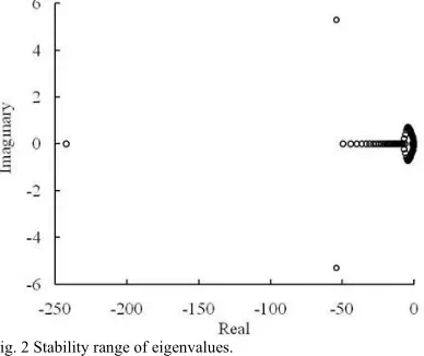
With the objective of customizing the numerical method to a non-uniform grid for strengthening numerical stability, a logical evaluation of the numerical method would consider its ranges of stability. The stability of a numerical method entails two facets, the temporal and spatial discretizations. Both aspects must be numerically stable. Mathematical theory decrees that the properties of the eigenvalues of a spatial discretization define its range of numerical stability [41]. The eigenvalue analysis begins with applying the numerical method, in this case, a 12th_{-order 5-point} non-uniform CCD scheme with 10th _{and 11}th_{-order boundary} schemes, to a reference governing equation, the classical one-dimensional convective diffusion equation. The theory mandates that the real part of the eigenvalue of the numerical discretization must be negative to ensure stability.

For the temporal discretization, the theory examines its amplification factor [41]. A temporal discretization will be stable if the absolute value of the amplification factor is less than one. Since the temporal discretization integrates the spatial discretization over time, the amplification factor is a function of the eigenvalue. This linkage allows for concurrent examination of the stabilities of both discretizations. The overall stability condition would require first that the real part of the eigenvalue be negative. Next, it selects the eigenvalues that limit the amplification factor to less than one.

Applying this two-step analysis to the one-dimensional convective diffusion equation indeed yields a set of eigenvalues for which the numerical method will remain stable, as depicted in Fig. 2. The stability of the numerical method when applied to this reference case provides indications as to how it will fare on the actual flow problem.

Fig. 2 Stability range of eigenvalues.

VIII. VALIDATION OF NUMERICAL METHOD The stable numerical method then must be validated for accuracy. An accurate numerical model would agree well with the Orr-Sommerfeld (OS) equation of linear stability theory. Figure 3 affirms agreement amongst the present study, three-dimensional OS equation, and numerical study of Fasel, et al., 1990 [42] for the downstream amplification rates of the disturbance velocities , , and :

ln (50)

where is the flow variable of interest. Figure 4 asserts

IAENG International Journal of Applied Mathematics, 42:2, IJAM_42_2_05

further averment with a near complete overlap between the present study and the OS equation for the transverse profiles of the disturbance velocities , , and . With confidence in the model accuracy, it is now ready for investigation of turbulence transition.

Fig. 3. Comparison of model, OS equation, and Fasel, et al., 1990 [42] for downstream amplification rates of velocities (a) , (b) , and (c) . Flow conditions given in Section III.

Fig. 4. Comparison of model results and OS equation for transverse profiles of disturbance velocities , , and .

IX. SUB-HARMONIC RESONANCE

The classical works Kachanov and Levchenko, 1984 [25] and Kachanov, 1994 [3] reveal the N-type turbulence transition involving sub-harmonic resonance of the propagating waves in ZPG boundary layer flow. The present study respectfully simulates the experiments in Kachanov and Levchenko, 1984 [25] using three Fourier modes in the spectral method with lowest wave number 31.47. The blowing and suction strip generates two-dimensional disturbances with = 12.4 and = 1.2 × 10-4 and three-dimensional disturbances with = 6.2 and = 5.1 × 10-6_.

Figure 5 shows comparison amongst the present study, Kachanov and Levchenko, 1984 [25], and numerical study of Fasel, et al., 1990 [42] for downstream amplification of

waves ⁄ / : modes (1, 0), two-dimensional initial TS waves, and (1/2, 1), subsequently generated three-dimensional sub-harmonic waves. The first entry in the brackets such as (1, 0) stands for multiples of the fundamental TS wave frequency, and the second entry represents multiples of the spanwise wave number. The three studies agree qualitatively. Figure 6 shows further close agreement amongst the three studies for the transverse profile of the wave amplitude for the mode (1, 0). The case for the mode (1/2, 1) in Fig. 7 displays less good agreement between the numerical studies and the experiments of Kachanov and Levchenko, 1984 [25].

Fig. 5. Comparison amongst present study, Kachanov and Levchenko, 1984 [25], and Fasel, et al., 1990 [42] for downstream amplification of waves: modes (1, 0) and (1/2, 1). Flow conditions given in Section III.

Fig. 6. Comparison amongst present study, Kachanov and Levchenko, 1984 [25], and Fasel, et al., 1990 [42] for transverse profiles of wave amplitudes of the mode (1, 0). Flow conditions given in Section III.

Fig. 7. Comparison amongst present study, Kachanov and Levchenko, 1984 [25], and Fasel, et al., 1990 [42] for transverse profiles of wave amplitudes of the mode (1/2, 1). Flow conditions given in Section III (% according to freestream velocity).

IAENG International Journal of Applied Mathematics, 42:2, IJAM_42_2_05

X. ASYMMETRICAL FLOW A. Full Fourier Expansion

Extension of the numerical model to investigate asymmetrical flows would logically follow. The previous assumption of symmetrical flow would no longer apply. So, instead of the compacted sine and cosine Fourier expansion of Eqs. (34) and (35), the spectral method must now use the full Fourier expansion of Eq. (33). Using Eq. (33), the governing equations become the following two sets. The first set of equations comprises [11, 37, 39]:

, (51)

, (52)

, (53)

, (54)

, and (55)

. (56)

The terms in Eqs. (51) to (56) with the subscript I are imaginary, while all the other terms are real. The second set comprises [11, 37, 39]:

, (57)

, (58)

, (59)

, (60)

, and (61)

. (62)

The terms in Eqs. (57) to (62) with the subscript R are real, while all the other terms are imaginary.

B. Adverse Pressure Gradient Flow Grid Independence Study

The numerical model of the present study with full Fourier expansion will simulate Borodulin, et al., 2002 [5]. The freestream velocity is given as:

H

H (63)

where H is the Hartree parameter fixed as −0.115 and is adjusted to 8.374 to match the flow conditions in Borodulin, et al., 2002 [5]. Figure 8 shows a comparison of the freestream velocity between the present study and Borodulin, et al., 2002 [5] with good overlap.

Fig. 8. Comparison of the freestream velocity between the present study and Borodulin, et al., 2002 [5].

Next, a grid independence test ensures that the numerical results would not be sensitive to the selection of grid spacing parameters. Table I gives the parameters used for two cases in the grid independence study. The test calibrates the initial disturbance strength at = 350 mm to match the experiments of Borodulin, et al., 2002 [5]. As such, the necessary initial amplitudes of fundamental and sub-harmonic waves are 0.1% and 0.01% of freestream velocity, respectively, corresponding to a disturbance frequency from the blowing and suction strip of 1.12 (109.1 Hz in experiments). Figure 9 shows the results for the transverse profile of the mean flow velocity using both grids along with the results of Borodulin, et al., 2002 [5]. Figure 10 shows the results for the downstream growth of the boundary layer thickness. Both figures exhibit complete overlap, indicating grid independence and concurrence with experimental data.

Table I. Computational parameters for grid independence study. The parameters m and n are the number of grids in the x- and y-directions, respectively and k is the number of Fourier modes used in the z-direction. X, Y, and Z are the physical dimensions in those directions.

m n k X(mm) Y(mm) Z(mm)

Case 1 280 60 4 200-760 0-17.4 0-48

Case 2 850 80 16 200-880 0-17.4 0-48

Fig. 9. Grid independence study for the transverse profiles of the flow velocity using a coarse grid (case 1), fine grid (case 2), and Borodulin, et al., 2002 [5].

IAENG International Journal of Applied Mathematics, 42:2, IJAM_42_2_05

Fig. 10. Grid independence study for the downstream growth of the boundary layer thickness using a coarse grid (case 1), fine grid (case 2), and Borodulin, et al., 2002 [5].

Sub-harmonic Resonance

The numerical model proceeds to simulate the sub-harmonic resonance of the generated waves in flow. Figure 11 shows the amplification of the wave amplitudes for the modes (1, 0) and (1/2, 1) with good agreement with Borodulin, et al., 2002 [5]. In Fig. 12, the transverse profiles of the wave amplitudes for the modes (1, 0) and (1/2, 1) once again agree with those of Borodulin, et al., 2002 [5].

Fig. 11. Amplification of the wave amplitudes for the modes (1, 0) and (1/2, 1) using a coarse grid (case 1), fine grid (case 2), and Borodulin, et al., 2002 [5].

Fig. 12. Comparison of transverse profiles of the wave amplitudes using a coarse grid (case 1), fine grid (case 2), and Borodulin, et al., 2002 [5]: (a) mode (1, 0) and (b) mode (1/2, 1).

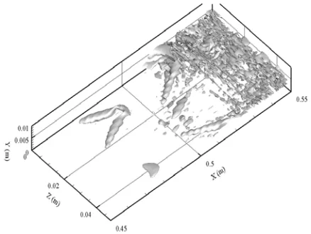
XI. TURBULENT STRUCTURE FORMATION In the alternative perspective, the aforementioned sub-harmonic resonance translates into the formation of definitive flow structures signaling the onset of turbulent transition. Section I describes these turbulent structures. Amongst them is the commonly observed Λ-vortex. Figure 13 confirms that the present study can capture the formation of the Λ-vortex when visualizing contours of the disturbance velocity ′ in the x-z plane. Interaction of the Λ-vortex with the high shear layer, another commonly observed structure, leads to the elongation of the tip of the Λ-vortex to form the Ω-vortex. Figure 14 captures the downstream development of the Λ-vortex using the Q-criterion technique of Jeong and Hussain, 1995 [43]. Indeed, the elongation towards an Ω -vortex is clearly evident.

Fig.13. Contours u’ in the x-z plane at y = 2.3 mm and t = 0.105 s.

Fig. 14. Vortex formation visualized at t = 0.105 s.

XII. BROADBAND DISTURBANCE FLOW A. Broadband Disturbance

More realistic turbulent conditions would entail a randomized disturbance. The present study continues by imposing a randomized signal from the blowing and suction strip shown in Fig. 1. Figure 15 shows the randomized disturbance amplitudes also known as broadband disturbance. The characteristics of the broadband disturbance is adopted from the experiments of Borodulin, et al., 2002 [5]. The size of the computational domain is 500 × 25.3 × 48 (mm) in the streamwise, transverse, and spanwise directions, respectively. The non-uniform grid generation uses parameters = 0.98 and = 30.16.

Figure 16 affirms once again good agreement between the present study and Borodulin, et al., 2002 [5] for the transverse profile of the amplitudes of ′. With confidence in the numerical model, it could proceed to investigate whether the coherent structures seen previously would persist in a randomized disturbance environment. Would there still be symphony in the midst of cacophony?

IAENG International Journal of Applied Mathematics, 42:2, IJAM_42_2_05

Fig. 15. Randomized disturbance introduced into the flow.

Fig. 16. Transverse profile of amplitudes of u’ at x = 450 mm, z = 14 mm.

B. Formation of Coherent Turbulent Structures

Λ-Vortex

The formation of the Λ-vortex indeed persists in the broadband disturbance flow as depicted in the evolutionary series from Figs. 17 a to d using the Q-criterion of Jeong and Hussain, 1995 [43]. The dark region below the Λ-vortex signals the formation of another flow structure known as the Soliton-like Coherent Structure (SCS).

(a)

(b)

(c)

(d)

Fig. 17. Evolution of Λ-vortex formation at (a) t = 0.061 s, (b) t = 0.0622 s, (c) t = 0.0635 s, and (d) t = 0.0649 s.

Streamwise Vortices

The legs of the Λ-vortices induce streamwise rotation commonly observed in boundary layer turbulence transitional flows [3, 25]. Visualizations of the flow vector field in the z-y plane at a downstream location x = 0.4323 m confirms the formation of streamwise vortices (see Fig. 18).

IAENG International Journal of Applied Mathematics, 42:2, IJAM_42_2_05

Fig. 18. Flow vector field with streamwise rotation at x = 0.4323 m and t = 0.053 s. The shaded contours represent u’.

Ω-Vortex

The flow structure evolution continues in Fig. 19. The tip of the Λ-vortex elongates and lifts up to form the Ω-vortex. Further elongation of the Ω-vortex results in its breaking away from the Λ-vortex to form a separated ringed vortex. Figure 20 shows the uplifting flow vectors that contribute to this sequence.

(a)

(b)

Fig. 19. Formation of Ω-vortex and subsequent break-off to form ringed vortex: (a) t = 0.066 s and (b) t = 0.0675 s.

Fig. 20. Flow vector field with upward lift at x = 0.4508 m and t = 0.059 s. The shaded contours represent u’.

Soliton-like Coherent Structure

The Λ-, Ω-, and ringed vortices interact with the SCS in interplay that would ultimately lead to flow randomization. The SCS is a persistent flow structure that resists breakdown by its surrounding flow. Figure 21 indeed depicts a powerful flow structure traversing along the wall region. The SCS plays a primary role in the evolution of the Λ- and Ω-vortices as can be seen in Figs. 17 and 19, as the SCS undergirds these structural formations.

Fig. 21. Flow vector field showing SCS at z = 0.0135 m and t = 0.053 s. The shaded contours represent u’.

Flow Randomization

The interplay amongst the Λ-, Ω-, and ringed vortices, as well as, with the SCS produces downstream flow randomization shown in Fig. 22. At this point the flow is turbulent. The nature of turbulence transition remains a mystery. The classical works of Klebanoff, et al., 1962 [24], Kachanov and Levchenko, 1984 [25], and Kachanov, 1994 [3] intimate that wave generation, amplification, and interaction dynamics lead to turbulence. Fourier decomposition of the flow velocity reveals five underlying harmonic waves shown in Fig. 23. The author predilects that perhaps their mysterious synchronization underlies the turbulence transition phenomenon.

IAENG International Journal of Applied Mathematics, 42:2, IJAM_42_2_05

Fig. 22. Evolution of Λ-, Ω-, and ringed vortices, as well as, with the SCS towards downstream flow randomization.

Fig. 23. Frequency spectrum disturbances measured at x = 450 mm.

XIII. CONCLUSION

This has been a study of sub-harmonic resonance in three-dimensional ZPG boundary layer flow. Sub-harmonic wave generation, amplification, and interaction drive the N-type pathway in turbulence transition made famous by the classical works of Kachanov and Levchenko, 1984 [25] and Kachanov, 1994 [3]. At the onset of turbulence transition, the wave dynamics become three-dimensional. Investigation of three-dimensional flows stands at the forefront of cutting-edge fluid dynamics research at the present time. Three-dimensionality incurs exorbitant computational demands on the numerical simulations that exponentially increase to impractical levels. The present study countervails such onerous computational demands by the imposition of a spectral method and a non-uniform grid. The symmetrical characteristic of the flow in the present study further improves upon the computational efficiency by needing only sine and cosine expansions in the spectral method, thereby reducing the computational demands by half. The non-uniform grid raises numerical stability issues at the wall boundary. Eigenvalue analysis ascertains ranges of stability of the numerical method. Validation of the

numerical method versus the three-dimensional OS equation avers confidence in the accuracy of the model. The present study respectfully emulates the classical experiments of Kachanov and Levchenko, 1984 [25]. The model simulations realize the resonance of the two-dimensional initial TS waves and the subsequently generated three-dimensional sub-harmonic waves with qualitative agreement to Kachanov and Levchenko, 1984 [25].

Extension of the numerical model to investigation of asymmetrical flows entails using the full Fourier expansion in the spectral method. Validation of the expanded model with Borodulin, et al., 2002 [5] affirms accuracy. The present study captures wave amplification dynamics for the modes (1, 0) and (1/2, 1) in good agreement with those of Borodulin, et al., 2002 [5]. A grid independence study proves that the numerical results do not depend on the specifications of the grid spacing.

Converting the input perturbation to a random signal adds closer verisimilitude to real turbulent flows. The commonly observed turbulent flow structures, Λ-, Ω-, and ringed vortices, manifest under these conditions also. Underlying mechanisms of streamwise vortices, upward lift away from the wall, and persistent SCS near the wall would appear to contribute to the observed structure formation. Ultimately, the turbulent structures break down into flow randomization. The author respectfully anthologizes his epistemology on the fascinating topic of turbulence transition in boundary layer flows. Chen, 2009 [26] invites readers to a bibliolatrous appreciation of the paper that has become the fulcrum for turbulent fluid dynamics research, Kolmogorov, 1941a [44], The Local Structure of Turbulence in Incompressible Viscous Fluid for Very Large Reynolds Numbers, better known as K41, which derives the very famous universal 5/3 law of Kolmogorov. A scholastic foray into the fundamental physics, mathematics, and numerical simulation of the Navier-Stokes equations and its variant form, the Vorticity Transport Equation, follows in Chen and Chen, 2010 [23]. The burgeoning study of the author logically proceeds into the numerical simulation of the linear stability stage of wave interactions leading to turbulence. Chen and Chen, 2009 [22] presents its findings at the 6th _{International Conference on Flow Dynamics,} Sendai, Japan and the 62nd _{Meeting of the Division of Fluid} Dynamics of the American Physical Society, Minneapolis, MN, USA. This stage signifies the completion of the fundamental background studies. Prior to investigating the question of interest, how flow becomes turbulent, Chen and Chen, 2012 [27] interlards a reportorial study of two very important preliminary issues of concern in the numerical simulation of turbulence transition: control of numerical errors and preservation of the generation, amplification, and interaction of microscopic-amplitude waves. Chen and Chen, 2010 [31] presents this work at the 7th _{International} Conference on Flow Dynamics, Sendai, Japan and 63rd Meeting of the Division of Fluid Dynamics of the American Physical Society, Long Beach, CA, USA. The contributions of the author to the field begins to receive recognition from the academic community beginning with Chen and Chen, 2011 [32], which further expands on the preceding work and makes presentation at the International Multi-Conference of Engineers and Computer Scientists 2011 where it earns the

IAENG International Journal of Applied Mathematics, 42:2, IJAM_42_2_05

distinction of the Best Paper Award. The scribomania continues in order to satisfy rising interest from the academic community with the invited paper, Chen and Chen, 2011 [28], and invited edited book chapter, Chen and Chen, 2012 [30]. The present study addresses the issue of turbulence transition in three-dimensional flows, a topic that lies at the forefront of contemporary research in the field. Chen and Chen, 2011 [33] presents this work at the 8th International Conference on Flow Dynamics, Sendai, Japan and 64th _{Meeting of the Division of Fluid Dynamics of the} American Physical Society, Baltimore, MD, USA. Copious details of that study resides in Chen and Chen, 2012 [29]. Chen and Chen, 2012 [34] presents this assiduous work at the International Multi-Conference of Engineers and Computer Scientists 2012. How does flow become turbulent? Knowledge of this profound question remains hitherto inchoate. Thank you for your consideration.

REFERENCES

[1] S. Bake, D. G. W. Meyer and U. Rist, “Turbulence mechanism in Klebanoff transition: A quantitative comparison of experiment and direct numerical simulation,” J. Fluid Mech., vol. 459, pp. 217-243, 2002.

[2] E. Mollo-Christensen, “Physics of turbulent flows,” AIAA J., vol. 9, no. 7, pp. 1217-1228, 1971.

[3] Y. S. Kachanov, “Physical mechanisms of laminar-boundary-layer transition,” Annu. Rev. Fluid Mech., vol. 26, pp. 411-482, 1994. [4] T. Herbert, “Secondary instability of boundary layers,” Annu. Rev.

Fluid Mech., vol. 20, pp. 487-526, 1988.

[5] V. I. Borodulin, V. R. Gaponenko, Y. S. Kachanov, D. G. W. Meyer, U. Rist, Q. X. Lian and C. B. Lee, “Late-stage transitional boundary-layer structures. Direct numerical simulation and experiment,”

Theoret. Comput. Fluid Dyn., vol. 15, no. 5, pp. 317-337, 2002. [6] C. B. Lee and J. Z. Wu, “Transition in wall-bounded flows,” Appl.

Mech. Rev., vol. 61, pp. 1-20, 2008.

[7] Z. Liu and C. Liu, “Fourth order finite difference and multigrid methods for modeling instabilities in flat plate boundary layers - 2-D and 3-D approaches,” Comput. Fluids, vol. 23, no. 7, pp. 955-982, 1993.

[8] D. R. Williams, H. Fasel and F. R. Hama, “Experimental determination of the three-dimensional vorticity field in the boundary-layer transition process,” J. Fluid Mech., vol. 149, pp. 179-203, 1984. [9] N. D. Sandham and L. Kleiser, “The late stages of transition to

turbulence in channel flow,” J. Fluid Mech., vol. 245, pp. 319-348, 1992.

[10] E. Laurien and L. Kleiser, “Numerical simulation of boundary-layer transition and transition control,” J. Fluid Mech., vol. 199, pp. 403-440, 1989.

[11] U. Rist and H. Fasel, “Direct numerical simulation of controlled transition in a flat-plate boundary layer,” J. Fluid Mech., vol. 298, pp. 211-248, 1995.

[12] H. L. Reed and W. S. Saric, “Stability of three-dimensional boundary layers,” Annu. Rev. Fluid Mech., vol. 21, pp. 235-284, 1989. [13] P. Andersson, L. Brandt, A. Bottaro and D. S. Henningson, “On the

breakdown of boundary layer streaks,” J. Fluid Mech., vol. 428, pp. 29-60, 2001.

[14] L. Kleiser and T. A. Zang, “Numerical simulation of transition in wall-bounded shear flows,” Annu. Rev. Fluid Mech., vol. 23, pp. 495-537, 1991.

[15] S. Biringen, “Final stages of transition to turbulence in plane channel flow,” J. Fluid Mech., vol. 148, pp. 413-442, 1984.

[16] S. Biringen, “Three-dimensional vortical structures of transition in plane channel flow,” Phys. Fluids, vol. 30, no. 11, pp. 3359-3367, 1987.

[17] R. G. Jacobs and P. A. Durbin, “Simulations of bypass transition,” J. Fluid Mech., vol. 428, pp. 185-212, 2001.

[18] D. Henningson and J. Kim, “On turbulent spots in plane Poiseuille flow,” J. Fluid Mech., vol. 228, pp. 183-205, 1991.

[19] M. T. Landahl, “Wave mechanics of breakdown,” J. Fluid Mech., vol. 56, no. 4, pp. 775-802, 1972.

[20] H. F. Fasel, U. Rist and U. Konzelmann, “Numerical investigation of the three-dimensional development in boundary layer transition ” in

19th AIAA Fluid Dynamics, Plasma Dynamics, and Lasers Conference, Honolulu 1987, pp. 12.

[21] G. Schubauer and H. K. Skramstad, “Laminar boundary layer oscillations and stability of laminar flow,” J. Aeronaut. Sci., vol. 14, no. 2, pp. 69-78, 1947.

[22] J. Chen and W. Chen, “Turbulence transition in two-dimensional boundary layer flow: Linear instability,” in 6th International Conference on Flow Dynamics, Sendai, Japan, 2009, pp. 148-149. [23] J. Chen and W. Chen, “The complex nature of turbulence transition in

boundary layer flow over a flat surface,” Intl. J. Emerging Multidisciplin. Fluid Sci., vol. 2, no. 2-3, pp. 183-203, 2010.

[24] P. S. Klebanoff, K. D. Tidstrom and L. M. Sargent, “The three-dimensional nature of boundary-layer instability,” J. Fluid Mech., vol. 12, no. 1, pp. 1-34 1962.

[25] Y. S. Kachanov and V. Y. Levchenko, “The resonant interaction of disturbances at laminar-turbulent transition in a boundary layer,” J. Fluid Mech., vol. 138, pp. 209-247, 1984.

[26] J. Chen, “The law of multi-scale turbulence,” Intl. J. Emerging Multidisciplin. Fluid Sci., vol. 1, no. 3, pp. 165-179, 2009.

[27] W. Chen and J. Chen, “Combined compact difference methods for solving the incompressible Navier-Stokes equations,” Intl. J. Numer. Methods Fluids, published online, 2012.

[28] J. Chen and W. Chen, “Two-dimensional nonlinear wave dynamics in blasius boundary layer flow using combined compact difference methods,” IAENG Intl. J. Appl. Math., vol. 41, no. 2, pp. 162-171, 2011.

[29] W. Chen and J. Chen, “Combined compact difference schemes on non-uniform grid for incompressible Navier-Stokes equations,” Intl. J. Numer. Methods Fluids, submitted, 2012.

[30] J. Chen and W. Chen, “Nonlinear wave dynamics in two-dimensional boundary layer flow,” in IAENG Transactions on Engineering Technologies, Vol. 7, S. Ao, A. Chan, H. Katagiri, L. Xu, Hong Kong: World Scientific, 2012, pp. 130-143.

[31] J. Chen and W. Chen, “Combined compact difference method for simulation of nonlinear wave generation, interaction, and amplification in boundary layer turbulence transition,” in 7th International Conference on Flow Dynamics, Sendai, Japan, 2010, pp. 82-83.

[32] J. Chen and W. Chen, “Numerical realization of nonlinear wave dynamics in turbulence transition using Combined Compact Difference methods,” in Lecture Notes in Engineering and Computer Science: Proceedings of The International MultiConference of Engineers and Computer Scientists 2011, Hong Kong, 2011, pp. 1517-1522.

[33] J. Chen and W. Chen, “Non-uniform grids in numerical simulations of boundary layer turbulence transition,” in 8th International Conference on Flow Dynamics, Sendai, Japan, 2011, pp. 168-169.

[34] J. Chen and W. Chen, “Sub-harmonic resonance in three-dimensional boundary layer flow,” in Lecture Notes in Engineering and Computer Science: Proceedings of The International MultiConference of Engineers and Computer Scientists 2012, Hong Kong, 2012, pp. 1635-1640.

[35] W. S. Saric, H. L. Reed and E. B. White, “Stability and transition of three-dimensional boundary layers,” Annu. Rev. Fluid Mech., vol. 35, pp. 413-440, 2003.

[36] S. A. Orszag and A. T. Patera, “Secondary instability of wall-bounded shear flows,” J. Fluid Mech., vol. 128, pp. 347-385, 1983.

[37] H. L. Meitz and H. F. Fasel, “A compact-difference scheme for the Navier-Stokes equations in vorticity-velocity formulation,” J. Comput. Phys., vol. 157, no. 1, pp. 371-403, 2000.

[38] C. Canuto, M. Y. Hussaini, A. Quarteroni and T. A. Zang, Spectral methods: Fundamentals in single domains. Berlin, Heidelberg: Springer-Verlag, 2006.

[39] C. Liu and S. A. Maslowe, “A numerical investigation of resonant interactions in adverse-pressure-gradient boundary layers,” J. Fluid Mech., vol. 378, p. 269-289, 1999.

[40] X. Zhong and M. Tatineni, “High-order non-uniform grid schemes for numerical simulation of hypersonic boundary-layer stability and transition,” J. Comput. Phys., vol. 190, no. 2, pp. 419-458, 2003. [41] C. Hirsch, Numerical computation of internal and external flows:

Fundamentals of computational fluid dynamics, 2nd edition. London: Butterworth-Heinemann, 2007.

[42] H. F. Fasel, U. Rist and U. Konzelmann, “Numerical investigation of the three-dimensional development in boundary-layer transition,”

AIAA J., vol. 28, no. 1, pp. 29-37 1990.

[43] J. Jeong and F. Hussain, “On the identification of a vortex,” J. Fluid Mech., vol. 285, pp. 69-94, 1995.

[44] A. N. Kolmogorov, “The local structure of turbulence in incompressible viscous fluid for very large Reynolds numbers,” Dokl. Akad. Nauk SSSR, vol. 30, no. 4, pp. 299-303, 1941.

IAENG International Journal of Applied Mathematics, 42:2, IJAM_42_2_05