Let the weekend begin!
A solution for solving the Weekend Scheduling Problem for ORTEC Harmony
Master thesis Industrial Engineering and Management Frédérique Versteegh
[email protected] June, 2009
Committee:
Dr. ir. E.W. Hans (University of Twente) Dr. ir. G.F. Post (University of Twente)
Drs. M. Hoogstrate (ORTEC)
University of Twente
School of Management and Governance
Starting to write your thesis feels like nishing a great period of life. Finishing writing your thesis feels like starting a new period in life. I thank all my friends and my family for the great experience that my student time was.
Graduation is sometimes a rough experience, but every rough moment forces you to learn and to grow. I thank ORTEC for oering me this research project and especially for the chance they have given me to go to Calgary. This was a very challenging and interesting experience in which ORTEC gave me the condence of successfully accomplishing the project. I thank my supervisor at ORTEC, Monique Hoogstrate, for her support, her critical views, the valuable lunch breaks, and for the nice period we have had. I thank my colleagues at ORTEC for their support, and especially my roommate, Egbert van der Veen, who I have bothered with many questions.
I thank my rst supervisor at the University of Twente, Erwin Hans, for his enthusiasm, his critical views, and for challenging me to a higher level. I thank Gerhard Post for his role as second supervisor.
Graduation knows some tough periods. I thank my boyfriend, Ralf Stamps, and my two dear friends, Golein Klein Bramel and Els Hettinga, for brightening me up in hard times and for not blaming me that I was not always in the best mood.
Last but not least, I thank my parents and my brothers for their support, the chances they have given me, and the freedom to explore.
To learn is to discover things of which you did not even know that you did not know them.
Management summary
Introduction
This research is performed within the Product Knowledge Center of ORTEC. ORTEC is one of the largest providers of advanced planning and optimization software solutions and consulting ser-vices. We study the assignment of weekend shifts in ORTEC's decision support software solution for workforce scheduling, called ORTEC Harmony. The assignment of weekend shifts is of great importance to customers, as weekends have an impact on the social life of employees and thus on employee satisfaction. In addition, unfullled demand in weekends is hard to cover and expen-sive, as irregularity allowances have to be paid for those hours. Harmony has the functionality to automatically create schedules. In a case study we analyze three real-life cases from practice that use this functionality. These customers use a two-step approach to schedule: weekend shifts as a priori step, followed by the remaining shifts. The current alternatives in Harmony to create satisfying schedules are very time-consuming. Even the best approach (varies per user) regularly leads to unfullled weekend demand and does not always satisfy user requirements. Users prefer an equitable schedule in which every employee works approximately the same number of weekend shifts and shift types.
Research objective
The objective of this research is to improve the assignment of weekend shifts such that unfullled demand is minimized and user requirements are satised as much as possible. The problem addressed by this objective is referred to as the Weekend Scheduling Problem.
Solution approach
We model the Weekend Scheduling Problem as a Quadratic Integer Programming model. For this problem we propose a stand-alone solution, the Weekend Planner. The Weekend Planner can be
embedded in Harmony, both as an individual planner and as an element of the current optimiza-tion engine. The Weekend Planner assigns weekend shifts to employees using an intelligent form of list scheduling. Working a shift means working a specic shift type in a specic weekend, for the whole weekend. For the selection of shifts and resources, the Weekend Planner uses selection rules based on exibility and busyness. First, the least exible shift is selected. In case of a tie, the shift is selected based on randomness. Second, the least busy and least exible resource is selected. Again, in case of a tie, the resource is selected based on randomness. Constraints on availability and on the maximum allowed number of weekends to work are taken into account. The creation of one schedule ends with a local search method. Random sampling is used to create diversity in the resulting schedules.
Results
The Weekend Planner is tested on three real-life cases from practice and on 400 random instances. Randomly generated instances with parameter ranges typically seen in practice are used to test the robustness and sensitivity of the Weekend Planner. Computational experiments show that the Weekend Planner solves 89% of the instances - i.e., all shifts are assigned - and solves 67.5% of the instances to optimality. The results deviate on average 3.8% from optimal. The Weekend Planner is most sensitive for cyclical schedules and schedules in which every employee needs to work its maximum number of weekends, in other words a tight schedule.
Computational experiments on the three real-life cases show that the Weekend Planner outper-forms Harmony on all aspects and improves schedules by 15% to 400%.
Conclusions
The Weekend Planner is a suitable method for solving the Weekend Scheduling Problem. The Weekend Planner decreases the unfullled demand and delivers more equitable schedules than Harmony does. The Weekend Planner focuses on weekend related constraints and therefore is a user-friendly and not time-consuming method.
Recommendations
1 Introduction 10
1.1 Context . . . 11
1.2 Problem description . . . 12
1.3 Research objective . . . 12
2 Context 15 2.1 Harmony's optimization engine . . . 15
2.1.1 Hard and soft constraints . . . 16
2.1.2 Model formulation . . . 17
2.1.3 Automatic planners . . . 19
2.1.4 Algorithm of Harmony's optimization engine . . . 20
2.2 Case study . . . 22
2.3 Performance and scheduling alternatives in Harmony . . . 24
2.3.1 Performance . . . 24
2.3.2 Alternatives to schedule weekend shifts in Harmony . . . 25
2.4 Requirements for Weekend Planner . . . 27
2.5 Related research . . . 28
3 Modeling 29 3.1 Modeling assumptions . . . 29
3.2 Mathematical problem denition . . . 30
3.3 Quadratic Integer Programming model . . . 32
CONTENTS 7
4 Weekend Planner design and description 35
4.1 Terminology . . . 35
4.2 Weekend Planner design . . . 35
4.3 Weekend Planner description . . . 36
4.3.1 Select shift . . . 38
4.3.2 Select resource . . . 39
4.3.3 Assign shift to resource . . . 40
4.3.4 Local search . . . 40
4.3.5 Sampling . . . 41
4.4 Alternative algorithm designs and model extensions . . . 41
4.4.1 Alternative algorithm designs . . . 41
4.4.2 Model extensions . . . 43
5 Computational results 45 5.1 Experiment approach . . . 45
5.2 Generation of random instances . . . 46
5.3 Test results on random instances . . . 47
5.4 Sensitivity analysis . . . 49
5.4.1 Algorithm settings . . . 49
5.4.1.1 Precision . . . 49
5.4.1.2 Number of samples . . . 54
5.4.1.3 Number of local search iterations . . . 54
5.4.2 Instance parameters . . . 55
5.4.2.1 Sensitivity of single parameters . . . 56
5.4.2.2 Combination of parameters . . . 56
5.5 Alternative algorithm designs . . . 57
5.6 Comparison results for case study . . . 59
5.6.1 Performance indicators . . . 59
5.6.2.1 Settings . . . 60
5.6.2.2 Calgary Health Region . . . 61
5.6.2.3 Belgian Police . . . 62
5.6.2.4 Kennemer Gasthuis Haarlem . . . 63
5.6.2.5 Conclusions on case study results . . . 64
5.6.3 Comparison Harmony results with Weekend Planner results . . . 65
6 Conclusions and recommendations 67 6.1 Conclusions . . . 67
6.2 Recommendations . . . 68
A Preliminary study - Calgary Health Region 71 A.1 Introduction to Calgary Health Region . . . 71
A.2 Process . . . 72
A.2.1 Current process . . . 72
A.2.2 Conclusion . . . 74
A.3 Control . . . 75
A.3.1 Harmony changes . . . 75
A.3.2 Denition of scheduling requirements in the software . . . 75
A.3.3 Conclusion . . . 76
A.4 Performance . . . 76
A.4.1 Quality of cyclical schedule . . . 76
A.4.2 Conclusion . . . 77
B Experimental results 79 C Sensitivity analysis 81 C.1 Instance size . . . 81
C.2 Availability . . . 83
C.3 Scope . . . 86
CONTENTS 9
C.5 Cyclical . . . 91
Introduction
This research describes improvements for a workforce scheduling algorithm that is used in a software solution for workforce scheduling called ORTEC Harmony (in the remainder called Harmony), a product of ORTEC. ORTEC is one of the largest providers of advanced planning and optimization software solutions and consulting services.
This research analyzes a problem in one of Harmony's modules: the optimization engine, which is used to automatically generate workforce schedules. First, it analyzes the current performance of Harmony regarding the planning of weekend shifts using a case study. The main current issues are inability to cover demand and to create an equitable division of weekend shifts. To solve these issues we propose a heuristic approach, the Weekend Planner, for the assignment of weekend shifts. The Weekend Planner consists of an intelligent form of list scheduling followed by a local search. The selection rules used in the list scheduling are based on selecting the least exible shift and the least exible resource. We describe the implementation of the Weekend Planner and test its robustness and the sensitivity of the solution. Finally, we compare the results of the Weekend Planner with Harmony's results for three real-life cases from practice.
Section 1.1 shortly describes the context in which this research has taken place and discusses ORTEC and Harmony. Section 1.2 describes the problem, followed by the research objectives and research questions in Section 1.3.
Context 11
1.1 Context
ORTEC
ORTEC is one of the largest providers of advanced planning and optimization software solutions and consulting services. ORTEC's solutions result in optimized eet routing and dispatch, vehicle and pallet loading, workforce scheduling, delivery forecasting and network planning. ORTEC has over 700 employees in several oces in Europe and North America and an extensive customer base in a large number of industries, including:
• trade, transport, and logistics
• oil, gas, and chemicals
• consumer packaged goods
• health care
• professional and public services
This research takes place at ORTEC's Product Knowledge Center (PKC) in Gouda, the Nether-lands. PKC transfers product knowledge and delivers nished products to market units and partners and is the link between ORTEC Software Development (OSD) and the market units. They are responsible for release management, documentation and trainings, product consultancy, and support. OSD also supports this research. OSD is responsible for developing and building ORTEC software.
Harmony
Harmony is an advanced planning solution for workforce scheduling. It is used in organizations that operate in an environment where work is carried out at irregular times and/or where the workload is uctuating during operating hours. Typical customers can be found in health care and in security industry. Harmony oers the possibility of creating shift rosters in a rapid and well-organized manner. One of its goals is to automatically generate the closest to optimal workforce schedules for a set of resources (employees) and a set of shifts, constrained by rules (hard constraints) and criteria (soft constraints).
in the software. In both ways the user is able to dene legislation, company specic rules, and regulations in the software. Harmony takes these into account to check if it is allowed to assign a shift to an employee on a certain day.
Harmony has two dierent types of schedules: cyclical schedules and non-cyclical schedules. Cyclical schedules are schedules repeating at regular intervals (i.e. every 4 weeks). A non-cyclical schedule is a schedule with a start and end date.
1.2 Problem description
The performance of the optimization engine does not meet several important requirements of some customers. In a case study (Section 2.2) we describe three customer situations, both cyclical and non-cyclical, and the problems they encounter when using the optimization engine. In that case study, the optimization engine appears not to be able to deliver schedules that meet or improve the quality of manually created schedules. ORTEC feels the need to investigate the abilities to improve the performance of the optimization engine. This results in the following problem description:
The optimization engine in Harmony does not meet all requirements regarding the assignment of shifts.
1.3 Research objective
Research objective 13
in the schedule. The general principle of Harmony is that the rst priority is to assign as many shifts as possible, while minimizing the penalties for soft constraints. Therefore, penalties on non-key performance indicators are of less importance in this research. This results in the following research objective:
Improve the assignment of weekend shifts for ORTEC Harmony, such that the total number of unassigned shifts and the penalties on key performance indicators are reduced.
To be able to achieve the research objective, this research investigates the following subjects:
• Context
1. How does the algorithm currently work in Harmony?
Description of the algorithm and current possibilities to plan in Harmony (Section 2.1).
2. What are the current problems with weekend shifts in more detail?
Analysis of three real-life cases from practice, performance, and scheduling alternatives (Sections 2.2 - 2.4).
• Model
1. What is the mathematical formulation of the problem?
Denition of the Weekend Scheduling Problem and a Quadratic Integer Programming formulation (Sections 3.1 - 3.3).
• Algorithmic improvements
1. What requirements should be considered when deciding on the algorithmic improve-ment?
Summarize found requirements in previous chapters (Section 4.2). 2. How can we solve the Weekend Scheduling Problem?
Description and design of the Weekend Planner (Chapter 4).
• Results
1. Is the solution robust?
2. How sensitive is the solution for various parameters?
Sensitivity analysis for algorithm settings and instance parameters (Section 5.4). 3. What is the performance result of implementing the improved algorithm, when testing
on the case study?
Analysis of Harmony's results compared with results of the Weekend Planner (Section 5.6).
Chapter 2
Context
This chapter discusses the context and some background information on this research. Section 2.1 explains how the optimization engine in Harmony currently works, including explanation of constraints, the dierent automatic planners available in Harmony, a model formulation, and the algorithm itself. Section 2.2 discusses a case study in which we analyze the problems regarding weekend shifts of three users of Harmony. Section 2.3 summarizes the current performance of the optimization engine and Section 2.4 describes the requirements for the solution. For information used in this chapter we refer to Fijn van Draat et al. (2005) and Van der Put (2005).
2.1 Harmony's optimization engine
The goal of the optimization engine of Harmony is to generate qualitatively good schedules, such that for as many shifts as possible the required number of employees is assigned, while all hard constraints and as many soft constraints as possible are satised. Hard constraints make schedules that do not satisfy these constraints infeasible; soft constraints act as quality measures for a schedule. Section 2.1.1 discusses the hard and soft constraints used in Harmony. Section 2.1.2 discusses the mathematical formulation of the workforce scheduling problem that Harmony solves. Section 2.1.3 explains the dierent automatic planners available in Harmony. Section 2.1.4 describes the algorithm of the optimization engine.
2.1.1 Hard and soft constraints
Numerous constraints are involved in personnel scheduling, both hard and soft constraints. Hard constraints impose rules on the schedule, making it infeasible when one of the hard constraints is violated. The optimization engine in Harmony never violates a hard constraint. The soft constraints are a measure for the quality of a schedule. Not satisfying a soft constraint increases the cost of the schedule, or in other words: imposes a penalty on the schedule (see formula (2.2) in Section (2.1.2)). In Harmony, the hard constraints are mostly incorporated in the so-called labor rules; the soft constraints are incorporated in the scheduling criteria (valid for all employees in the schedule) and work agreements (apply to individual employees).
Hard constraints
The hard constraints can be divided into four categories:
1. Legislation: these constraints apply to all employees. Examples of these constraints are:
• A maximum of xhours of work in y week(s)
• In x days there should be a period of rest of at leasty hours
• After a night shift the rest time should be at least x hours
2. Industry agreements, such as collective labor agreements: these constraints apply to all em-ployees that work in the sector or industry for which the agreement has been set. Examples of these constraints are:
• At least x weekends o in a period of y weeks
• A weekend o is dened as a time slot of at least x hours without labor, including
Saturday 00:00 AM until Monday 04:00 AM.
3. Organizational/departmental level: extra constraints can be dened within an organization or a department. An example of such a constraint is:
• At most x shifts of work in a row
4. Personal level: constraints that only apply to certain employees, based on their individual contract or requests. Examples of these constraints are:
Harmony's optimization engine 17
• An employee can only work shifts of type xand y
• An employee can only work shifts for which he is qualied
The constraints mentioned above are just examples for the specic categories, some constraints can appear in more categories with dierent parameter values. For example, legislation can subscribe a maximum number of 60 hours per week, but for the specic industry rules may say that a lower maximum number of 50 hours per week applies.
Soft constraints
The soft constraints can be divided into the following three categories:
1. Organization or department criteria: these apply to all employees of the organization/department. Examples of these criteria are:
• No stand-alone shifts
• In a weekend assign either no, or otherwisex shifts
2. Group criteria: apply to certain groups of employees, such as part-time employees. Exam-ples of these criteria are:
• Shifts series should be between x andy shifts for employees workingv to z hours per
week
• At least x shifts of type y in a period of w weeks for employees workingv to zhours
per week
3. Individual criteria: preferences of individual employees, such as:
• Employee x prefers shift y on dayz
2.1.2 Model formulation
criterion (how much over or under the dened criterion boundaries) and on the way the severity is calculated (depending on the criterion the excess is taken linearly or quadratically). The severity thus diers every time a criterion is broken. An example of severity is when the criterion describes a maximum of 4 shifts in a row and 6 shifts in a row are planned, then the criterion is exceeded by 2 shifts. If the excess of this criterion is taken quadratically, the severity is 4.
The value of the cost function is the weighted sum of the unsatised soft constraints. A qualita-tively good schedule is a schedule with a minimum number of unassigned shifts and an objective value of the cost function that has a minimum amount of penalties given the number of unas-signed shifts. We call a schedule an individual, the objective is to improve the score of that individual. The score of an individual consists of the penalties per resource and the penalties for the unassigned shifts. The weight used for the criterion that involves the unassigned shifts is usually set to 1,000,000, whereas weights for other criteria are in the range of 1 to 1,000. This section discusses the problem description of Harmony's workforce scheduling model. First we introduce some notation:
• R is the set of resources (employees), r is an element of the set if r∈R
• S is the set of shifts, s is an element of the set ifs∈S
• C is the set of criteria, c is an element of the set ifc∈C
• wc is the weight assigned to criterion c
• wcu is the weight for an unassigned shift (= 1.000.000)
• ςc is the severity of how criterion c is not met
• ϕ(r, c) =
ςc if resource r violates criterion c
0 otherwise
• ϕ˜(s) =
1 if shift s is unassigned
0 otherwise
The cost function per resourcef(r) can be dened as:
f(r) =X
c∈C
wc·ϕ(r, c) (2.1)
Harmony's optimization engine 19
Shift Sequence Planner
Optimization Engine Vacant Shifts
Planner
Greedy insertion Local search
Greedy insertion
Genetic algorithm Local search VNS Calls in Harmony
Calls in Harmony Calls in Harmony
C
a
lls
C
al
ls
User
Figure 2.1: Relation between automatic planners in Harmony
dened as:
Score Individual=−X
r∈R
X
c∈C
wc·ϕ(r, c) −
X
s∈S
wcu·ϕ˜(s) (2.2)
2.1.3 Automatic planners
Harmony contains three dierent automatic planners:
• Shift Sequence Planner: the user denes possible shift sequences: a consecutive combination
of shifts that occur often, i.e. DDDD (four day shifts in a row) or DDEE (two day shifts followed by two evening shifts). This planner tries to schedule as many shift sequences against the lowest possible cost, using a greedy insertion followed by a local search.
• Vacant Shifts Planner: assigns the unassigned shifts using a greedy insertion. This planner
sorts the unassigned shifts based on several criteria and assigns each shift to the best available resource (based on cost function) for which the rules are not violated. This Vacant Shifts Planner does not reconsider assigned shifts.
• Optimization engine: optimization engine with a genetic algorithm and a local optimizer
that generates a complete schedule. Section 2.1.4 describes the algorithm of the optimization engine in more detail.
2.1.4 Algorithm of Harmony's optimization engine
This section discusses the algorithm of Harmony's optimization engine's, which consists of three steps:
1. Genetic algorithm
2. Local optimization
3. Variable Neighborhood Search (VNS)
The philosophy behind this algorithm is twofold:
• robust - the algorithm is robust for instance characteristics (input data) and problem
de-nitions (changing constraint and/or criteria set);
• control possibilities - the planner can adjust weights for criteria etc.
The remainder of this section describes the three steps of the algorithm.
Genetic algorithm
The rst phase of the algorithm consists of a genetic algorithm. A genetic algorithm is a ran-domized search process based on the principles of natural evolution and 'survival of the ttest'. For general information on genetic algorithms we refer to Goldberg (1989). The rst step of the algorithm is to generate an initial population, called generation 0. The user sets a value for the number of individuals in the population that has to be created. Harmony uses the Vacant Shifts Planner to create generation 0. To make sure to get dierent unique individuals, the algorithm divides the resources randomly in two groups and uses the Vacant Shifts Planner to rst assign as many shifts as possible to the resources of the rst group and then assigns as many remain-ing shifts as possible to the resources of the second group. This procedure is repeated until the algorithm has created enough unique individuals for generation 0.
Harmony's optimization engine 21
1-opt move 2-opt move 1- opt- 2 move 2- opt- 2 move
Figure 2.2: 1-opt and 2-opt moves
the next generation. This process of creating generations continues until no further improvement is found during a certain period.
Local optimization
Once the global optimization stops, the algorithm continues with a local search consisting of a 1-opt and 2-opt search on the best schedule found in the genetic algorithm. A 1-opt move (Figure 2.2) takes one shift and assigns it to the rst feasible resource that is better than the current assignment. A 2-opt move consists of selecting two shifts that are currently assigned to dierent resources. If exchanging them is feasible and results in an improvement, the exchange takes place. The schedule is said to be 1-optimal when the schedule cannot be improved by a 1-opt change. When the schedule is 1-optimal the algorithm starts a 2-opt search. When it nds one 2-opt improvement, the algorithm returns to the 1-opt search, until the schedule is 1-optimal again. When the schedule is also 2-optimal, the algorithm starts a 1-opt-2 search: a 1-opt search in which 2 shifts are moved to another resource. The algorithm returns to the 1-opt-1 search every time an improvement is found, it continues the local search until it reaches a 2-opt-3 optimal schedule, or until no further improvements can be found within a reasonable amount of time.
Variable Neighborhood Search
Solution space
Local optimum
Kick to other neighborhood
Figure 2.3: Variable Neighborhood Search
algorithm continues until the time set by the user is spent or until an optimal solution is found, in other words when a schedule is found with a value 0 for the objective function as described in formula 2.2. When the value of formula 2.2 is 0, the schedule has no unassigned shifts and violates no soft constraints.
2.2 Case study
Appendix A describes a preliminary study performed at a customer of Harmony: Calgary Health Region (CHR). CHR uses a new module in Harmony: the optimization engine for cyclical sched-ules. In this study the problem of assigning weekend shifts as described in Chapter 1 rst became clear. This section summarizes their problems with respect to weekend shifts. To test whether this performance problem only appears in the new functionality, this section also discusses two cases of other ORTEC customers that use the optimization engine for non-cyclical schedules: the Belgian police and a Dutch hospital, the 'Kennemer Gasthuis Haarlem'.
Calgary Health Region
Case study 23
do not want employees to work only a Saturday or only a Sunday. In the current performance of Harmony single weekend shifts sometimes are assigned. A third problem is that the assignment of weekend shifts is not equitable, not regarding the amount of the same shift types and not regard-ing the number of weekends an employee works. This last problem arises especially when more employees than weekend shifts are available, in which case the weekend shifts are not divided equally over all employees. This results for example in one employee working three weekends and somebody else working only one weekend. It is neither equitable when one employee works two weekends of night shifts and another employee works two weekends of day shifts.
Belgian Police
The Belgian Police also uses the optimization engine in Harmony to schedule their employees. They use non-cyclical schedules. The problems they encounter when making schedules are com-parable to those at Calgary Health Region: not all shifts are assigned to employees, not every employee works the same number of weekend shifts, and employees get assigned single weekend shifts. The rst problem arises especially when employees already have for example a vacation, training, or occasional activities (such as alcoholic beverage control) scheduled in the scheduling period, so more constraints are placed on that resource. They also want an equitable division of the types of shifts to be worked among employees. Their workaround to create reasonable sched-ules is to use the Shift Sequence Planner and manual tweaking for the weekend shifts followed by the optimization engine to schedule the remaining shifts. Nevertheless, this workaround does not solve all problems mentioned before. They still encounter diculties to divide weekend shifts equally over employees when they already have leave scheduled in the scheduling period. They use dierent rules than Calgary Health Region when scheduling for weekends; all rules that do not directly inuence weekend shifts are turned o. They do use rules to stimulate an equitable division of the number of shifts and shift types.
Kennemer Gasthuis Haarlem
they see as an important disadvantage.
2.3 Performance and scheduling alternatives in Harmony
Section 2.3.1 summarizes the current performance of Harmony's automatic planners. Section 2.3.2 summarizes the possibilities currently available in Harmony to schedule weekend shifts.
2.3.1 Performance
From the case study we derive four major problems with respect to scheduling weekend shifts in Harmony. The optimization engine does not always:
1. schedule all weekend shifts, whereas a feasible solution does exist for all weekend shifts.
2. divide the weekend shifts equitably over all employees: not all employees work the same number of shifts and shift types during weekends.
3. assign either zero or two shifts in a weekend.
4. assign two shifts of the same type in a weekend.
Performance and scheduling alternatives in Harmony 25
Shift 1 Unassigned Shift 1 Shift 2 Resource X
Day Z
Empty Resource Y
Empty Unassigned
Shift 1 Resource X
Day Z
Shift 2 Resource Y
Figure 2.4: A 3-opt change in which an unassigned shift gets assigned
A 3-opt change for example, could give a better result, as Figure 2.4 shows, but unfortunately Harmony's local search does not include 3-opt. Because of the quality of the start solution for the local search, the local search has to make a too large improvement.
Problems 2, 3, and 4 are problems the optimization engine simply does not take into account if the user does not dene soft constraints for these subjects. In the three cases described in Section 2.2 the users did dene the corresponding constraints, but as they are soft constraints, Harmony can, and obviously does, violate them. This shows that solving problem 2, 3, and 4 by dening soft constraints is not sucient for the users of the optimization engine.
2.3.2 Alternatives to schedule weekend shifts in Harmony
The previous sections show that the performance of the optimization engine is not sucient for weekend shifts. Scheduling all shifts in one step is too complicated. Fortunately, the optimization engine as explained above is not the only possibility in Harmony to plan weekend shifts. This section summarizes the current possibilities in Harmony to schedule weekend shifts.
Calgary Health Region
Belgian Police
Kennemer
Gasthuis Average
Penalty increase with weekend shifts as a priori
step
12% 4.6% 2.5% 6.4%
Remaining non-weekend shifts with weekend shifts as
a priori step
1.7% 1.5% 1.3% 1.5%
Remaining weekend shifts with non-weekend shifts as a
priori step
40% 29% 50% 40%
Table 2.1: Comparison of results for weekend shifts as a priori step to non-weekend shifts as a priori step
Unassigned shifts on weekend days are of more inuence to a company than unassigned shifts on non-weekend days. It is hard (nobody wants to give up a free weekend) and expensive (pay irregularity allowances) to get these unassigned shifts lled. Next, the assignment of weekend shifts has the most inuence on the social life of employees. To keep your employees satised, it is important to schedule weekend shifts as much as possible according to employee preferences.
We thus conclude that a two-step approach with scheduling weekend shifts as an a priori step is the best scheduling method. For this a priori step Harmony has several options:
• Optimization engine for weekend shifts only
Requirements for Weekend Planner 27
• Optimization engine for weekend shifts only with non-weekend rules and criteria turned o
The user denes rules and criteria for a schedule. Some of these rules and criteria do not concern weekend shifts. Although these rules do not directly concern weekend shifts, the planner checks on them. It might have a positive inuence on the resulting schedule when these rules are turned o during the assignment of weekend shifts. Further advantages and disadvantages are equal to the option above.
• Shift sequence planner
The user predenes shift sequences. For weekend shifts they start on Friday or Saturday and consist of 2 or 3 consecutive shifts. The shift sequence planner tries to assign as many shift sequences as possible to resources. The user can predene the priority of a sequence and whether that sequence is valid for the whole department or only for selected employees. The advantage of this option is that for weekends only sequences are scheduled that the user wants, so no single weekend shifts and no consecutive shifts of dierent shift types (unless the user prefers so). The disadvantage is that this option does not try to divide the shifts equally over all employees. The user can dene criteria to stimulate an equitable division, but again, these are soft criteria and thus not always met.
• Plan manually
A last option to improve a schedule is to tweak manually. Users often (if not always) make manual adjustments after using one of the above described options to improve the resulting schedule and adjust it to their preferences.
2.4 Requirements for Weekend Planner
This section discusses which requirements the Weekend Planner has to satisfy. These requirements can be split into two parts: general requirements, resulting from within ORTEC, and requirements for the resulting schedules of the Weekend Planner, which follow from the users of the optimization engine.
The main general requirements for the Weekend Planner are:
• Implementation: it has to be possible to implement the solution in the current structure of
Harmony.
• Generic: over 200 customers use Harmony and they all have to be able to work with the
perception is that the problem occurs at many customers. This emphasizes the need for a generic solution.
• No workarounds: as described in Section 2.2 several users of the optimization engine
cur-rently use workarounds to create reasonable schedules. Workarounds are available in Har-mony, but as the problem is generic, it is important to come up with a solution that makes workarounds unnecessary. The Weekend Planner nally has to become part of a one-step-scheduling process for the user.
The main requirements for the resulting schedules of the Weekend Planner are:
• All weekend shifts assigned to employees, if a feasible solution exists;
• Weekends divided equitably over all employees;
• No stand-alone weekend shifts;
• The same shift-type for all shifts in one weekend.
2.5 Related research
Chapter 3
Modeling
This chapter describes the mathematical model of the problem discussed in this research. Section 3.1 gives the assumptions of the model, Section 3.2 describes the mathematical problem denition, followed by a quadratic integer programming model in Section 3.3.
3.1 Modeling assumptions
As with every translation of real life situations into a mathematical model, several assumptions have to be made. Assumptions can also be useful to decrease the problem size and to keep the problem from becoming too complicated. This section describes the assumptions we make for the problem as described in Chapter 2.
• we only consider the planning of weekend shifts in this research. This planning of weekend
shifts is a pre-processing of the planning of the complete schedule;
• all employees cost the same, i.e. wages are not taken into account;
• demand for shifts is equal on Saturdays and Sundays;
• in the model we use weeks as indices for time, the week represents a complete weekend;
• if a resource works in a certain week in the model, he works both on Saturday and on
Sunday and the same shift type on both days;
• a shift is a period of work, for example a morning assignment from 7 AM - 3 PM, or an
afternoon assignment from 1 PM - 9 PM etc.
We realize that the above list is not complete; factors like contract hours and age related require-ments are not taken into account in this stage of the research. We will discuss some important possible extensions of the model in Section 4.4.2.
3.2 Mathematical problem denition
This section starts by introducing the sets we use in the remainder of this research:
Sets
R resources (index r)
W weeks (index t)
W+ subset of W,={t≥0}
S shift types (index s, z)
In the remainder of this research we will use shift as a unique combination of a week and a shift type:
Denition 3.1. Shift(s,t)
Shift(s,t) is the unique combination of shift type s in week t.
Mathematical problem denition 31
Denition 3.2. (Weekend Scheduling Problem)
GIVEN: A nite set of time periods W, a set of resources R, a set of shift types S, the following
parameters:
dts demand: number of resources needed for shift(s,t)
arts
(
1 if resource r is available for shift(s,t) (vacation, skills, etc.)
0 otherwise
wer maximum number of weekends resourcer can work in wr weeks
wr number of weeks in which resource r can workwer weekends,
qrt
(
1 if resource r works in week t (t<0 )
0 otherwise
and the following decision variables
Xrts
(
1 if resource r works shift type s in week t
0 otherwise t= 0, . . . , W
Crts
(
1 if resource r is allowed to work shift type s in week t
0 otherwise
GOAL: Does there exist a binary vectorx = (Xrts), such that the deviation between the number
of weekends a resource works and the average workload per resource, and the deviation between the number of shifts a resource works of each allowed shift type is minimized (an equitable division of weekend assignments over the resources) for cyclical schedules (variant a) and non-cyclical schedules (variant b) and such that the following constraints, of which the mathematical formulation is given in Section 3.3, hold:
• demand dts is satised in every week tfor every shift types(constraint 3.4);
• every resource works at most one shift type per week (constraint 3.5);
• every resource only works shifts that it is allowed to work (constraint 3.6);
• every resource works maximum wer weekends in wr weeks (constraint 3.8a for cyclical
schedules and constraint 3.8b for non-cyclical schedules).
3.3 Quadratic Integer Programming model
This section describes a quadratic integer programming formulation (QIP) of WSP (Denition 3.2). First, we discuss the formulation of the objective function, followed by the formulation of the complete model and the explanation of the constraints.
Objective function
The objective function consists of two parts. The rst part establishes a minimization of the dif-ference between the number of weekends a resource works and the average workload per resource. This dierence is taken quadratically because a deviation of 4 for one resource is worse than a deviation of 1 for four resources for example. This rst part of the objective is as follows:
minX
r
X
t,s
Xrts−
P
t,s
dts
|R|
2
(3.1)
The second part of the objective function consists of the minimization of the deviation from an equitable division of shift types for each resource. The goal of this objective is to make sure that each resource works approximately the same number of weekends of each shift type that that resource is allowed to work. For example, two resources working both one weekend with day shifts and one weekend with night shifts is preferred over one resource with two weekends of night shifts and the other resource working two weekends of day shifts.
This deviation is formulated as the dierence in the number of weekends worked between all
possible combinations of shift typessandzfor each resource. We only take the value of a worked
weekend with shift type s into account if the resource would have been allowed to work shift
typez as well. To accomplish this, we multiply variableXrtswith the parameter for availability
for shift type z: artz and vice versa. To make sure we take all possible combinations of shift
types into account, we compare for each resource the number of weekends worked with shift type
s to the number of weekends worked with shift type z, if the ordinality of z is larger than the
ordinality ofs. As the deviation consists of positive and negative deviation, we need to take the
absolute value:
minX
r
X
s,z|ord(s)<ord(z)
X
t
(artz·Xrts−arts·Xrtz)
(3.2)
Quadratic Integer Programming model 33
zrsz+ Assisting variable for the positive deviation from an equitable division of shift types
sandz for resourcer
zrsz− Assisting variable for the negative deviation from an equitable division of shift types
sandz for resourcer
Next, we introduce two extra constraints to make sure that z+
rsz and z−rsz represent the positive
respectively negative deviation:
zrsz+ ≥X
t
(artz·Xrts−arts·Xrtz) ∀r, s, z
zrsz− ≥X
t
(arts·Xrtz−artz·Xrts) ∀r, s, z
and to make sure that for each resource only one of the two assisting variables gets a nonzero value:
zrsz+ ≥0 ∀r, s, z
zrsz− ≥0 ∀r, s, z
Now we can replace formula (3.2) by the following linear minimization:
min X
r
X
s,z|ord(s)<ord(z)
zrsz+ +zrsz−
The two parts of the objective function are not equally important. The equitable division of the number of shifts is most important. An increase in penalty for the division of the number of shifts over an equal decrease in penalty for the division of shift types should be prevented. That
is why we give both parts of the objective function a weight, α (for the part on the division of
the number of shifts) andβ (for the part on the division of shift types), where αis larger thanβ.
QIP formulation
The preceding sections lead to the following QIP formulation for the Weekend Scheduling Prob-lem:
minX
r
α·
X
t,s
Xrts−
P
t,s
dts
|R|
2
+β· X
s,z|ord(s)<ord(z)
z+rsz+zrsz−
s.t. X
r
Xrts ≥ dts ∀t, s (3.4)
X
s
Xrts ≤ 1 ∀r, t (3.5)
Xrts ≤ Yrts ∀r, t, s (3.6)
Crts ≤ arts ∀r, t, s (3.7)
(t+wr−1)mod|W|
X
τ=t
X
s
Xrτ s ≤ wer ∀r, t (3.8a)
(t+wr−1)
X
τ=t (X
s
Xrτ s) +qrτ
≤ wer ∀r, t=−wr+ 1, . . . ,
W+
−wr+ 1 (3.8b)
z+rsz ≥ X
t
(artz·Xrts−arts·Xrtz) ∀r, s, z (3.9)
z−rsz ≥ X
t
(arts·Xrtz−artz·Xrts) ∀r, s, z (3.10)
z+rsz ≥ 0 ∀r, s, z (3.11)
z−rsz ≥ 0 ∀r, s, z (3.12)
Xrts ∈ {0,1} ∀r, t, s (3.13)
Constraints (3.4)-(3.8b) describe the constraints as given in Denition 3.2. Constraint (3.4) enforces that the demand is met. Constraint (3.5) forces a resource to work maximal one shift per day. Constraint (3.6) assures that a resource only works the types of shifts it is allowed to work. Constraint (3.7) makes sure that resources are only allowed to work a shift if they were
available for that shift according to parameter arts. Constraints (3.8a)/(3.8b) make sure that
Chapter 4
Weekend Planner design and
description
This chapter proposes a solution to solve the WSP: the Weekend Planner. Section 4.1 explains some of the terminology used. Section 4.2 discusses the main considerations in designing the Weekend Planner. Finally, Section 4.3 describes the proposed heuristic.
4.1 Terminology
In this chapter we use the denitions of weeks and shift types as used earlier in this research. So by a week we mean a complete weekend. By a shift(s,t) we mean the unique combination of a week and a shift type. A resource is an employee who can work shifts. The goal is to assign shifts to resources according to the WSP with its constraints as described in Chapter 3.
4.2 Weekend Planner design
This section summarizes the main insights for solution design from Chapter 2. Creating a schedule in one integral step is too complicated (as results in Section 5.6.2 also show). Users of Harmony's optimization engine currently schedule in two sequential steps. The best scheduling sequence has shown to be scheduling weekend shifts as a priori step (see Section (2.3.2)), followed by the remaining, non-weekend shifts. For the a priori step various methods are used, ranging from manual scheduling to using one of Harmony's automatic planners or a combination of methods. They schedule the remaining shifts with Harmony's optimization engine. This two-step approach
results in a satisfying schedule according to users, but the a priori step is labor-intensive. As Harmony's optimization engine is suitable for the scheduling of the non-weekend shifts, we focus on a new method for the a priori step: the Weekend Planner.
The Weekend Planner has to take the following objectives into account in lexicographic order of importance:
1. create an assignment of weekend shifts with zero remaining shifts (if possible)
2. create an assignment of weekend shifts with an equitable division of the number of weekends worked
3. create an assignment of weekend shifts with an equitable division of shift types
Because of the way we have modeled the WSP, the Weekend Planner automatically takes the following two requirements, which also follow from Chapter 2, into account:
• create an assignment of weekend shifts without stand-alone weekend shifts
• create an assignment of weekend shifts with consecutive shifts of the same shift type
As the current possibilities in Harmony do not focus on the above objectives, this research pro-poses a solution that is not based on the current structure of the available algorithms in Har-mony. We propose a heuristic approach, the Weekend Planner, which uses an intelligent form of list scheduling to select shifts and to assign them to resources. The Weekend Planner assigns shift(s,t) to an employee, which means that if an employee works shift(s,t), the employee works shift type s on Saturday and Sunday of the corresponding week t. List scheduling takes objective 2 into account if the selection rules are set up accordingly. To meet objective 1, the Weekend Planner will schedule the least exible shifts and the least exible resources rst. List scheduling does not take objective 3 into account. Therefore the last step of the Weekend Planner is a local search with the objective to improve the equality of the division of shift types.
4.3 Weekend Planner description
This section describes the following steps of the Weekend Planner (Algorithm 4.1) for one solution in more detail:
Weekend Planner description 37
Algorithm 4.1 Weekend Planner for Number of Samples
while (remainingShifts > 0) and (availableResources > 0) Select shift
Select resource
Assign shift to resource Update availability Check weekend constraint end
Local search
if Solution is better than BestSolutionSoFar BestSolutionSoFar := Solution
end end
• Select resource (Section 4.3.2)
• Assign shift to resource (Section 4.3.3)
• Local search (Section 4.3.4)
Because of randomness in the Weekend Planner, we apply a sampling technique, which we explain in Section 4.3.5.
The Weekend Planner uses selection rules for the construction of a solution. To make sure that the largest number of shifts is scheduled, it is important to schedule the least exible shifts and the least exible resources rst. The last shifts to schedule are the shifts with the most exibility. Flexibility depends on the total number of comparable shifts that still have to be scheduled, and on the number of resources that are still available for that shift. The least exible shift is assigned to the least exible resource. Flexibility of resources depends on the number of shifts already assigned to a resource in the planning period and on the number of shifts a resource is available for. We only take feasible shift-resource combinations into consideration.
4.3.1 Select shift
The Weekend Planner uses the following rules in decreasing order of importance to select shift(s,t):
1. Shift(s,t) with the lowest exibility ratio: "unfullled demand for shift(s,t)/ remaining avail-able resources"
shift(s,t) for which
P
r
Xrts−dts
P
r
Yrts is minimal.
The shift that this rule selects is the least exible shift, because for this shift less resources are available than for all other shifts. So this shift is the hardest shift to plan and for this reason has to be assigned to a resource rst.
This rule results in a tie when two ratios are equal. Note: both are rounded on k decimals; k is an experimental factor.
2. Shift(s,t) with the smallest number of shifts still to be scheduled:
shift(s,t) for which
dts−P
r
Xrts
is minimal.
If the rst rule results in multiple possible shifts, the shift(s,t) with the smallest absolute number of shifts to be scheduled is selected. For example: take shift(A,1)(shift type A in week 1) and shift(B,1)(shift type B in week 1). For shift(A,1) still 2 shifts have to be assigned and there are 4 available resources. For shift(B,1) still 20 shifts have to be assigned and there are 40 available resources. Both shifts have a exibility ratio of -0.5, but assigning shift(A,1) is less exible than assigning shift(B,1), so shift(A,1) is selected.
3. Select rst shift in time line
From the remaining shifts, this rule selects the shift that is closest to the start of the planning period. This is important because resources have a history, so the weeks closest to the previous planning period are more inuenced by this history than weeks more to the end of the planning period. Shifts close to the start of the planning period are less exible than shifts later in the planning period, due to more constraints on the number of weekends that still can be worked.
4. Select random shift
Weekend Planner description 39
4.3.2 Select resource
The Weekend Planner uses the following four rules in decreasing order of importance to select a resource for the selected shift(s,t) :
1. "Least busy resource": resource with lowest number of weekends scheduled in scheduling period:
resource for which P
t,s
Xrts is minimal.
This rule makes sure that each resource is assigned to approximately the same number of weekends, as is stated in the objective function of the WSP. The resource with the lowest number of assigned shifts is chosen.
2. "Least exible resource": resource with lowest number of available shifts that the resource is allowed to work :
resource for which P
t,s
Yrts·
dts−P
r
Xrts
is minimal.
A resource that is allowed to work ten of the available shifts (shifts still to be scheduled) is more exible than a resource that is allowed to work only four available shifts. The number of shift types a resource is allowed to work inuences this rule, but also the number of weeks a resource has requested vacation for. This rule selects the least exible resource.
3. Resource for which the exibility ratio of the least exible other shift(s,t) that that resource is allowed to work in the same week t as the selected shift(s,t), is maximal. This rule nds for each resource the least exible shift that that resource is allowed to work in week t, except for the selected shift. This rule then selects the resource(s) for which the least exible shift is most exible (of all found least exible shifts). This is thus the resource for which the other shifts that that resource can work, have the most exibility, so the Weekend Planner does not lose much exibility with assigning the selected shift to this resource. The other shifts this resource could work in the same weekend are the 'easiest' to plan, as their ratio is maximal. This rule selects:
resource for which min
s|Yrts=1
P
r
Xrts−dts
P
r
Yrts is maximal for given t of selected shift(s,t).
and shift(C,1). The exibility ratio for shift(B,1) is -0.3 and for shift(C,1) -0.2. Shift(B,1) is thus harder to assign than shift(C,1). So resource 1 is more 'needed' for shift(B,1) than resource 2 is 'needed' for shift(C,1). It is more exible to assign shift(A,1) to resource 2 in this step.
4. Select random resource
If the above rules result in multiple resources, select a random resource from the remaining resources.
4.3.3 Assign shift to resource
Once a resource has been selected, the selected shift is assigned to the selected resource. The
availability variable Crts is updated for resource r after every assignment of shift(s,t) to that
resource. The availability for the selected resource is set to 0 for all shift types in the week of the selected shift. Next, the algorithm performs a check on the number of weekends a resource works to check on the weekend constraint (constraints 3.8a/3.8b in Section 3.3) and adjusts the availability parameter if necessary.
The process of selecting shifts and resources continues until all shifts have been assigned to resources, or until no more shifts can be assigned to resources.
4.3.4 Local search
The Weekend Planner stimulates an equitable division of the number of shifts. Thus far, it does not focus on an equitable division of shift types. Therefore, we perform a 2-opt local search to improve the division of shift types. The 2-opt local search included in the Weekend Planner evaluates shift swaps for each combination of two assigned shifts in the same week. The swap is made if it results in a lower value of the objective function and thus in a more equitable division of shift types (Algorithm 4.2).
Alternative algorithm designs and model extensions 41
Algorithm 4.2 2-opt Local Search included in the Weekend Planner
While (improvement found in last iteration) and (NoIterations<MaxIterations) for all Weeks
for every 2 resources that work in the same week, but dierent shift types
if resources are allowed to work each others shift type Exchange shifts and calculate new score
if new score < current score then keep exchange else change shifts back
end end end end end
4.3.5 Sampling
As there is a random component in the construction algorithm, not every solution for an instance has to be the same. One solution might be better than another, generated with other random values. The Weekend Planner creates a solution a number of times (as requested by the user) and selects the best solution to give back as output. This process is called random sampling (Kolisch and Drexl, 1996). As randomness only aects the last selection rule of both shift and resource, the inuence of randomness and thus of sampling might be small. Chapter 5 addresses the inuence of randomness and analyzes various number of samples to determine the best scenario.
4.4 Alternative algorithm designs and model extensions
This section discusses some alternative designs of the Weekend Planner (Section 4.4.1). Next, the Weekend Planner is a generalized form of the cases that occur in practice. Section 4.4.2 summarizes a few extensions that frequently occur and the way they can be included in the Weekend Planner.
4.4.1 Alternative algorithm designs
Take random shift in time
This could result in problems towards the end of the planning period. Chapter 5 addresses the consequences of excluding this rule.
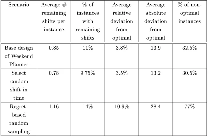
Regret-based random sampling
Regret-based random sampling (RBRS) is a randomized construction heuristic often used in scheduling, proposed by Kolisch and Drexl (1996). This method uses priority rules to value solution building blocks. In the Weekend Scheduling Problem the shifts and resources are the solution building blocks, and for example the exibility of a shift determines the priority of that shift. Instead of simply selecting the building block with the highest priority, this method calculates a probability for each building block based on its priority. The higher the priority, the higher the probability of a building block is. RBRS then selects a building block from all candidates, using their probabilities. This method also uses sampling (see Section 4.3.5).
This method calculates priority vj for building block j using a priority rule. The user denes
the priority rule. Given a priorityvj, we calculate the regret factorrj, which is the non-negative
dierence of the priorityvj and the worst of all building block priorities:
rj =vj −min
i {vi}, if a high v implies a high priority
rj =max
i {vi} −vj, if a high v implies a low priority
The higher the regret factor rj is, the more regret you have of not selecting the building block.
Based on the regret factor we calculate the probability Pj of a solution building block being
drawn:
Pj =
(rj + 1)γ
P
i
(ri+ 1)γ (4.1)
The parameter γ is the so-called bias-factor. the larger γ is chosen, the larger the eect of the
regret factor is.
As an alternative design, we apply regret-based random sampling to the Weekend Scheduling Problem, based on the selection rules of the Weekend Planner. We adjust the described general form of RBRS to be suitable for the WSP. We calculate a separate probability for the selection of a shift and for the selection of a resource. We here describe the method to select a shift, the same holds for resource selection. The probability in the standard RBRS is based on only one priority rule. The Weekend Planner uses various priority rules to select a shift. We calculate the regret and probability per shift per priority rule as in the general RBRS. This results in three
Alternative algorithm designs and model extensions 43
of shift selection sum up to 1. We then multiply each weight with the corresponding probability and sum these values for all three priority rules:
Ps =
X
i
wi·Pi
Each shift then has one probability Ps, based on which a shift is selected. The priorities of all
shifts obviously sum up to 1.
The standard formula to calculate a probability (formula 4.1) increases the regret with 1, such that each building block has a nonzero probability of being drawn. The Weekend Planner contains selection rules in which priority and regret are based on the exibility ratio of shifts. The regret is thus always < 1. Increasing the regret with 1 would destroy the proportion between the probabilities for dierent shifts, as this increase is larger than the regret itself. For priority rules based on ratios (the rst shift selection rule and the third resource selection rule) we increase the regret with 0.01 instead of 1 preventing a destruction of proportions, but maintaining a nonzero probability for each building block:
Pj =
(rj+ 0.01)γ
P
i
(ri+ 0.01)γ
The selection rules that the Weekend Planner uses are dened as consecutive rules. RBRS uses priority rules as independent rules. Consecutive rules are not necessarily suitable for independent use. The second shift selection rule selects the shift(s,t) with the smallest number of shifts still to be scheduled, if the rst rule (select the least exible shift(s,t)) results in a tie. Independently, the second rule does not make sense: the shift(s,t) with the smallest number of shifts still to be scheduled should not get a high priority. We thus set the weight of this priority rule for use in RBRS to 0.
4.4.2 Model extensions
FTE (Full Time Equivalent) The Weekend Planner stimulates an equitable division of the absolute number of shifts. However, when not all resources work the same FTE, users might prefer to divide the weekends in proportion to the FTE. To accomplish this, the rst rule to select a resource has to be changed to : resource for which
P
t,s
Xrts
F T E is minimal.
the Weekend Planner, the availabilityartshas to be set to 0 for resourcer for alltand for all shift
typessthat are night shifts. To include a maximum number of night shifts, an extra constraint
Chapter 5
Computational results
This chapter describes the results for the Weekend Planner. Section 5.1 gives the experiment approach and a further outline of this chapter.
5.1 Experiment approach
The experiment consists of the following steps:
1. Determine the best scenario of the Weekend Planner:
(a) Test Weekend Planner on a diverse set of random generated instances (Section 5.2 and 5.3)
(b) Analysis of the sensitivity of the Weekend Planner for various parameters (Section 5.4):
i. Algorithm settings ii. Instance parameters
(c) Test alternative designs (Section 5.5)
2. Test the best scenario of the Weekend Planner on three real-life cases from practice and compare these results with Harmony's results (Section 5.6)
5.2 Generation of random instances
For the tests we use randomly generated test instances. To generate these instances we rst randomly assign shifts to employees. Second, we choose the instance parameters such that the assignment of shifts to employees is optimal. Third, we calculate the objective value for this instance.
1. Randomly assign shifts to employees
We create a large number of employees and randomly assign shifts to them. In this way we have created many dierent employees/schedules of which we can choose some that form a feasible and optimal schedule in the next step.
2. Choose instance parameters such that schedule is optimal
(a) We randomly choose instance parameters. See Table 5.1 for these parameters and the possible values. These bounds are based on values that occur often in practice. The scope is dened as the maximum number of weekends an employee is allowed to work in a period (thus dened as x out of y weeks). The tightness is dened as the ratio of the number of weekends an employee has to work over the maximum number of weekends an employee is allowed to work. From the tightness we can thus calculate the number of weekends that each employee should work if each employee works the same number of shifts.
Parameter Values
Number of employees [10..70]
Number of weeks [4,6,8,10,13]
Scope [1/2 , 2/4 , 3/4 , 2/5]
Tightness [1/max ..1]
Cyclical [true, false]
[image:46.612.157.472.479.583.2]Number of shift types [1..6]
Table 5.1: Parameter settings for testing random instances
Test results on random instances 47
number of shifts and equality in the division of shift types. Equality in the division of the number of shifts is assured because every employee works the same number of weekends: the chosen value in step (a). Equality in the division of shift types is assured because only employees are selected that work the same number of shifts of every shift type (or one more of some shift types when the number of shift types is not a multiple of the number of weekends every employee works).
(c) Based on the assigned shifts, we calculate the corresponding demand. To make the instance more realistic, not all employees are available for all shifts (i.e. in case of vacation). For every shift(s,t) that an employee does not work in the created schedule, the availability of the employee for that shift is randomly set to 0 (not available) or 1 (available). The randomness of the availability is inuenced by an instance parameter, a randomly chosen value between 0 and 1 that gives the probability of employees in that instance being available for a shift.
3. Calculate objective value for instance
Now that all parameters are chosen such that the schedule is optimal, we can calculate the objective value. As we know that the schedule is optimal, we thus know the optimal value for this instance. The next section compares the results of the Weekend Planner with the optimal value.
5.3 Test results on random instances
This section evaluates the results of the Weekend Planner on random instances on the following performance indicators:
• Deviation from optimal solution
For each instance the absolute as well as the relative deviation from the optimal solution is measured. The results also show the average over a large number of instances of the absolute and relative deviation from optimal. The deviation is the dierence between the test result and the optimal solution according to formula 3.3.
• Remaining shifts
Setting Value
Precision 1
Number of samples 20
Local search iterations 5
α (weight on rst part objective function) 2
[image:48.612.178.450.113.200.2]β (weight on second part objective function) 1
Table 5.2: Algorithm settings for tests on the Weekend Planner
We use 400 random instances, for which we know the optimal solution. The number of 400 is selected based on preliminary tests that show the average deviation from the optimal solution becoming a at and stable line with 400 instances.
Table 5.2 illustrates the settings used to test the Weekend Planner. The values forα and β are
found by tests that are not illustrated here. Section 5.4.1 analyzes the sensitivity of the Weekend Planner for the other settings.
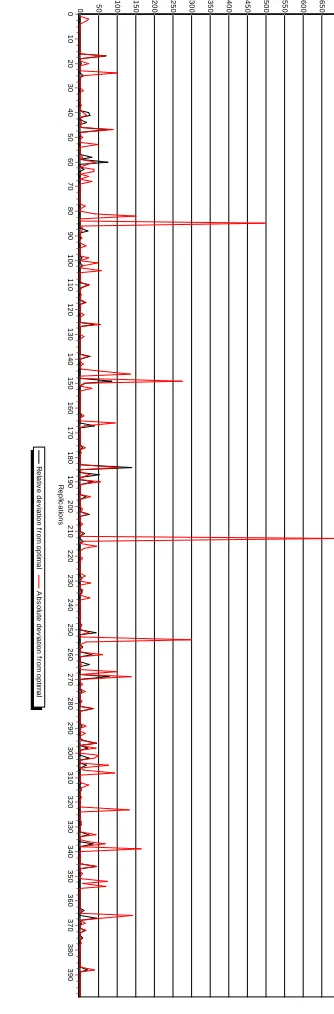
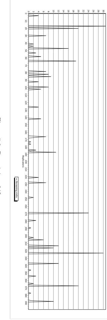
Deviation from optimal solution
Figure 5.1 shows the absolute and relative deviation from the optimal solution for each of the 400 instances. In 67.5% of these instances the Weekend Planner has found the optimal solution.
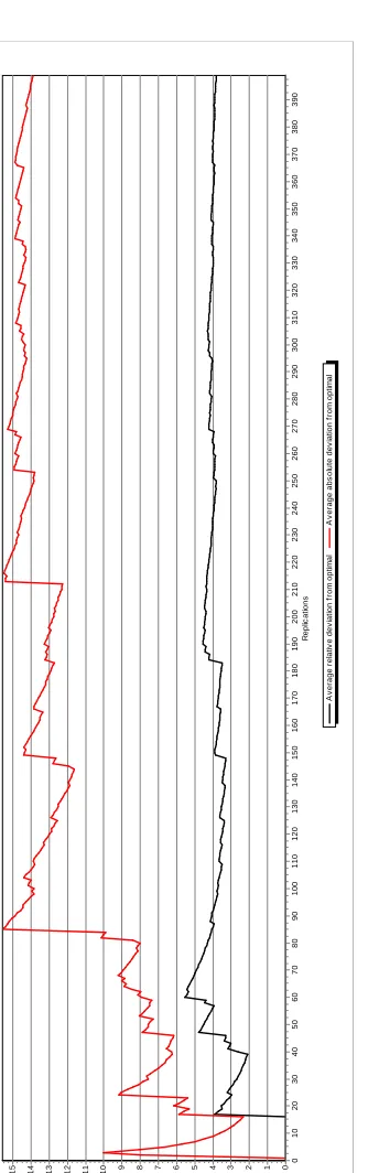
Figure 5.2 shows the average absolute and relative deviation from the optimal solution. The average absolute deviation is 13.9; the average relative deviation is 3.8% from optimal. The gures show that for some cases the deviation from optimal is very high. This deviation is mainly caused by a non-equitable division of shift types. Figure B.1 in appendix C shows the total penalty, the penalty for an equitable division of the number of shifts, and the penalty for an equitable division of shift types. This gure shows that the graph for the total penalty is equal or quite close to the penalty for an equitable division of shift types for all instances. In the optimal solution every employee works exactly the same number of shifts, which means that the penalty for an equitable division of the number of shifts is 0. When the total penalty in the Weekend Planner is equal to the penalty for the equitable division of shift types, we know that the division of the number of shifts is optimal.
Sensitivity analysis 49
extensive local search, as is already available in Harmony, decreases the penalty for an equitable division of shift types and so decreases the deviation from optimal.
Remaining shifts
Figure 5.3 shows the number of remaining shifts for each instance. For 89% of the instances the Weekend Planner has found a solution with 0 remaining shifts. The average number of remaining shifts is 0.85 shift per instance (measured over all 400 instances). For some instances the number of remaining shifts is quite high. The sensitivity analysis in Section 5.4.2 analyzes the inuence of the dierent instance parameters on the results of the Weekend Planner and the possible causes for high remaining shifts.
5.4 Sensitivity analysis
This section analyzes the sensitivity of the Weekend Planner for variation in the algorithm settings (Section 5.4.1) and for the dierent values of instance parameters (Section 5.4.2).
5.4.1 Algorithm settings
This section analyzes the sensitivity of the Weekend Planner for the following algorithm settings:
• Precision parameter k (Section 5.4.1.1)
• Number of samples (Section 5.4.1.2)
• Number of iterations in the local search (Section 5.4.1.3)
For each of these settings, we analyze the inuence of dierent values for a setting on the number of instances with remaining shifts, the average number of remaining shifts per instance, the number of instances for which the Weekend Planner nds the optimal solution, and the average deviation from the optimal solution.
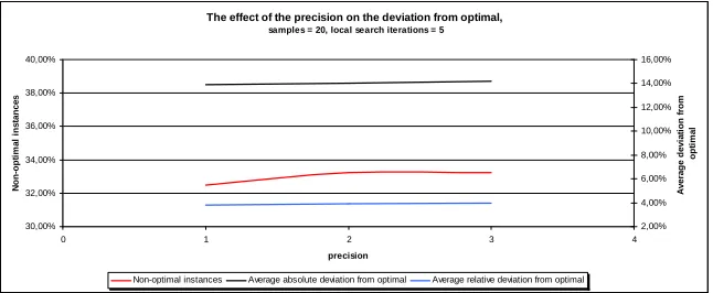
5.4.1.1 Precision
Sensitivity analysis 51 A v e ra g e r e la ti v e d e v ia ti o n f ro m o p ti m a l A v e ra g e a b s o lu te d e v ia ti o n f ro m o p ti m a l R e p lic a ti o n s 3 9 0 3 8 0 3 7 0 3 6 0 3 5 0 3 4 0 3 3 0 3 2 0 3 1 0 3 0 0 2 9 0 2 8 0 2 7 0 2 6 0 2 5 0 2 4 0 2 3 0 2 2 0 2 1 0 2 0 0 1 9 0 1 8 0 1 7 0 1 6 0 1 5 0 1 4 0 1 3 0 1 2 0 1 1 0 1 0 0 9 0 8 0 7 0 6 0 5 0 4 0 3 0 2 0 1 0 0 1 5 1 4 1 3 1 2 1 1 1
0 9 8 7 6 5 4 3 2 1 0
[image:51.612.206.378.165.697.2]Sensitivity analysis 53
The effect of the precision on the deviation from optimal,
samples = 20, local search iterations = 5
30,00% 32,00% 34,00% 36,00% 38,00% 40,00%
0 1 2 3 4
precision N o n -o p ti m a l in s ta n c e s 2,00% 4,00% 6,00% 8,00% 10,00% 12,00% 14,00% 16,00% A v e ra g e d e v ia ti o n f ro m o p ti m a l
[image:53.612.140.463.115.248.2]Non-optimal instances Average absolute deviation from optimal Average relative deviation from optimal
Figure 5.4: The eect of precision on the deviation from optimal
The effect of the precision on remaining shifts,
samples = 20, local search iterations = 5
8,00% 10,00% 12,00% 14,00% 16,00% 18,00% 20,00%
0 1 2 3 4
precision In