Using Sparse Semantic Embeddings Learned from Multimodal Text and Image Data to Model Human Conceptual Knowledge

260

Using sparse semantic embeddings learned from multimodal text and

image data to model human conceptual knowledge

Steven Derby1 _{Paul Miller}1 _{Brian Murphy}1,2 _{Barry Devereux}1

1 _{Queen’s University Belfast, Belfast, United Kingdom} 2 _{BrainWaveBank Ltd., Belfast, United Kingdom}

{sderby02, p.miller, brian.murphy, b.devereux}@qub.ac.uk

Abstract

Distributional models provide a convenient way to model semantics using dense embed-ding spaces derived from unsupervised learn-ing algorithms. However, the dimensions of dense embedding spaces are not designed to resemble human semantic knowledge. More-over, embeddings are often built from a sin-gle source of information (typically text data), even though neurocognitive research suggests that semantics is deeply linked to both lan-guage and perception. In this paper, we com-bine multimodal information from both text and image-based representations derived from state-of-the-art distributional models to pro-duce sparse, interpretable vectors usingJoint Non-Negative Sparse Embedding. Through in-depth analyses comparing these sparse models to human-derived behavioural and neuroimag-ing data, we demonstrate their ability to pre-dict interpretable linguistic descriptions of hu-man ground-truth sehu-mantic knowledge.

1 Introduction

Distributional Semantic Models(DSMs) are used to represent semantic information about concepts in a high-dimensional vector space, where each concept is represented as a point in the space such that concepts with more similar meanings are closer together. Unsupervised learning algorithms are regularly employed to produce these models, where learning depends on statistical regularities in the distribution of words, exploiting a theory in linguistics called the distributional hypothe-sis. Recent developments in deep learning have resulted in weakly-supervised prediction-based methods, where, for example, a neural network is trained to predict words from surrounding con-texts, and the network parameters are interpreted as vectors of the distributional model (Mikolov et al., 2013). Like their counterparts in machine vision, neural network algorithms for DSMs au-tomate feature extraction from highly complex

data without prior feature selection (Krizhevsky et al., 2012;Mikolov et al., 2013; Karpathy and Li, 2015; Antol et al., 2015). Such deep learn-ing techniques have led to state-of-the-art perfor-mance in many domains, though this is often at the expense of the interpretability and cognitive plausibility of the learned features (Murphy et al.,

2012; Zeiler and Fergus, 2013). Furthermore, these compact, dense embeddings are structurally dissimilar to the way in which humans conceptu-alise the meanings of words (McRae et al.,2005). One way of drawing interpretability from highly latent data is by transforming it into a sparse repre-sentation (Faruqui et al.,2015;Senel et al.,2017). Moreover, the design of distributional models has been for the most part unimodal, typically relying on text corpora, even though studies in psychol-ogy have shown that human semantic processing is deeply linked with visual perception.

In cognitive neuroscience, research demon-strates that representations of high-level concepts corresponding to the meanings of nouns and vi-sual objects are widely distributed and overlapping across the cortex (Haxby et al., 2001; Devereux et al., 2013), which has opened up research into exploiting machine learning for neurosemantic prediction tasks using distributed semantic mod-els (Mitchell et al.,2008;Huth et al.,2016;Clarke et al.,2015;Devereux et al.,2018). Such research has helped with both the construction and eval-uation of semantic distributional embeddings in computer science (Devereux et al.,2010;Søgaard,

se-mantics as exhibited in human cognitive knowl-edge and neurocognitive processing, when com-pared with dense embeddings learned from the same data.

2 Related Work

Much of the research aimed at the sparse decom-position of dense vector spaces is closely asso-ciated with the work of Hoyer (2002), who pro-posed aNon-Negative Matrix Factorization tech-nique(NMF) known asNon-Negative Sparse Cod-ing (NNSC) which produces a sparse represen-tation of the original compact matrix. With the use of new optimisation techniques (Mairal et al.,

2010),Murphy et al.(2012) later implemented a variation of this approach that forces an L1 penalty on the new sparse matrix, yieldingNon-Negative Sparse Embedding (NNSE). The purpose of the NNSE algorithm is to generate an embedding that attains the desirable qualities of effectiveness and interpretability (Murphy et al. (2012)). Building upon this approach, Fyshe et al. (2014) extended NNSE to incorporate other sources of semantic in-formation using an extension of NNSE known as Joint Non-Negative Sparse Embedding(JNNSE). Their experiments made use of neuroimaging data as an additional source of semantic information, and recent work has seen a push for the incorpo-ration of a broader range of semantic knowledge into DSMs, including semantic knowledge derived from visual image information.

Bruni et al. (2014) combined embeddings from text and co-occurrence statistics from data via mining techniques derived from pictures us-ing a procedure known as Visual Bag-of-Words (VBOW). Later this approach was extended by

Kiela and Bottou (2014) who incorporated the penultimate layer of modified Convolutional Neu-ral Networks (CNN) to forge a more grounded, semantically faithful model that improved on the state-of-the-art. Lazaridou et al. (2015) extend the architecture of the skip-gram model associated with Word2Vec (Mikolov et al.,2013) to incorpo-rate a measure of visual semantic information by forcing the network to learn linguistic and visual-based features. Instead of performing a context-based prediction task, Ngiam et al. (2011) com-bine multimodal information from both audio and image-based information using a stacked autoen-coder to reconstruct both modalities with a shared representation layer in the middle of the network.

Modality Source Embeddings #D #S

Text GloVe 1000 200

Text Word2Vec 1000 200

Image CNN-Mean 6144 1000

Image CNN-Max 6144 1000

Both CNN-Mean + GloVe 7144 200 Both CNN-Max + GloVe 7144 200 Both CNN-Mean + Word2Vec 7144 200 Both CNN-Max + Word2Vec 7144 200

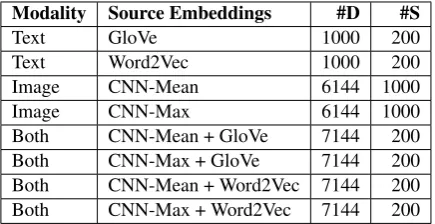
Table 1: List of all dense (D) and sparse (S) models used in this paper, and the number of dimensions (#) in each model.

Silberer et al. (2017) similarly combine informa-tion from multiple modalities from both visual and linguistic data sources by using a stacked au-toencoder to reconstruct both types of informa-tion separately with a shared representainforma-tion layer, and a softmax layer connected to the representa-tion layer used to predict the concept characterised by these representations. Rather than trying to construct each modality separately, Collell et al.

(2017) make use of a simple perceptron and a neu-ral network to reconstruct the visual modality from pretrained linguistic representations.

3 Multimodal Representation

In total, we used sixteen distributional seman-tic models, eight of which are dense and eight of which are their sparse counterparts. These models are summarized in Table 1, which de-scribes the eight sources of semantic information (two text-based, two image-based, and four mul-timodal image+text-based) used to construct both the dense and sparse embedding models. Con-struction of the eight dense models largely fol-lowed Kiela and Bottou (2014), with eight cor-responding sparse models later constructed using JNNSE.

3.1 Text-based models

We implemented two state-of-the-art text-based embedding models, Word2Vec and GloVe, to act as initialisers for our sparse models, following a similar approach to Faruqui et al. (2015). Both text-based models were trained on 4.5 gigabytes of preprocessed Wikipedia data, with fixed context windows of size 5 and 1000 embedding dimen-sions. The Wikipedia preprocessing was standard and included removal of Wikipedia markup, stop words and non-words, as well as lemmatisation (implemented using standard NLTK tools). Af-ter model training, the embeddings for each word were normalised to mean zero and unit length, us-ing the L2 norm. Vector normalisation was carried out to ensure magnitudes of the text-based vectors were in line with the image-based vectors, which are normalised by default.

GloVe. Global Vector for Word Representa-tion (Pennington et al., 2014) is an unsupervised learning algorithm that captures fine-grained se-mantic information using co-occurrence statistics. It achieves this by constructing real vector embed-dings using bilinear logistic regression with non-zero word co-occurrences in the training corpus within a specific context. Our model was trained using a learning rate of0.05over100epochs.

Word2Vec. Word2Vec (Mikolov et al., 2013) uses shallow neural networks with negative sam-pling techniques, which are trained to predict ei-ther the word from the context or the context from the word using a fixed window of words as the context. In particular, we choose the CBOW ver-sion (predict the word using the context) of this model which was trained using thegensim pack-age with the minimum word count threshold set to

0(i.e., a vector representation was created for all

words in the corpus).

3.2 Image models

We make use of the image embeddings con-structed byKiela and Bottou(2014). In their pa-per, the AlexNet (Krizhevsky et al., 2012) CNN was extended from1000output units to1512 out-puts, using the additional 512 object label cate-gories chosen byOquab et al.(2014) and retrained using transfer learning (Oquab et al.,2014). This new network was trained using the 2012 version of the ImageNet Large Scale Visual Recognition Challenge(ILSVRC) competition dataset with ex-tra images from 512other categories, which was then later used to gather embeddings for the ESP game image dataset (Von Ahn and Dabbish,2004). After training, the network was sliced to remove the final fully-connected softmax layer, in order to retrieve the activation vectors for each image on the penultimate layer. There are systematic differences in the kinds of images that appear in the ImageNet and ESP game training sets. The ImageNet dataset (Deng et al., 2009) consists of

12.5million images over22K different object cat-egories, with each image typically corresponding to a single labelled object (i.e. images do not tend to be cluttered with several objects). In contrast, the ESP game dataset consists of 100000images with many labelled objects present in each image. To retrieve activation vectors for object cate-gories from the ESP dataset, Kiela and Bottou

(2014) used a fair proportional sampling tech-nique: for each object category label,1000images were sampled according to the WordNet (Miller,

1995) subtree for that concept. If sampling up to1000images was not possible, then the subtree of the concepts hypernym parent node was further sampled until1000images were retrieved. The ac-tivation vector for each of these images was then obtained from the truncated CNN. To retrieve the final embedding vectors for each object label from the sampled activation vectors, Kiela and Bottou

(2014) combined the 1000 activation vectors for each label using two techniques, described below. CNN-Max. Each word embedding was pro-duced by taking the elementwise maximum value over all 1000 CNN activation vectors obtained for the sampled images with the same label word.

label word.

All image embeddings are of size6144, corre-sponding to the size of the penultimate layer of the CNN. The embeddings used in our paper cor-respond to the ESP game labels (which uses a larger number of images, more natural images, and more labels than ImageNet), and all embeddings are normalised to mean zero and L2 unit length before downstream analysis.

3.3 Multimodal models

Again followingKiela and Bottou(2014), we pro-duce four new dense models from combinations of text and image embeddings by simply concatenat-ing the embeddconcatenat-ing vectors of each model corre-sponding to each word to create new multimodal text+image embeddings:

V ecmulti =α×V ectext||(1−α)×V ecimage

(1) Here,αis a mixing parameter that determines the relative contribution of each modality to the com-bined semantic space. We setα= 0.5, so that text and image sources contribute equally to the com-bined embeddings.

4 Sparse matrix factorization

FollowingFaruqui et al.(2015), we use the dense text and image model embeddings as initialisers for corresponding sparse embedding spaces. The embedding vectors are concatenated into an em-bedding matrix for each model, with the number of rows corresponding to the number of words in their respective lexicons, and the number of columns corresponding to the embedding dimen-sionality.

To produce the new sparse representations, we use the NNSE matrix factorisation technique 1 (Murphy et al.(2012)) which maps a dense word-feature matrix X to a non-negative sparse matrix A with an identical lexicon. Let X ∈ Rw×k be

an embedding matrix, where w is the number of words, and k is the embedding dimension size. NNSE factorisesXinto two matrices, a dictionary transformation matrixD ∈ _Rp×k _{and the sparse}

matrix A ∈ _Rw×p _{by minimising the objective}

function:

argmin D,A

w

X

i=1

||Xi,:−Ai,:×D||2+λ||Ai,:||1 (2)

1_{Non-Negative Sparse Embedding code was kindly}

pro-vided by Partha Talukdar.

subject to the constraints

Di,:DTi,:≤1,∀1≤i≤p Ai,j ≥0,∀1≤i≤w,∀1≤j≤p

which ensure sparse and non-trivial solutions for A(Murphy et al.(2012)).

NNSE has been extended as a method to com-bine multiple dense word-feature matrices X ∈ Rwx×k and Y ∈ Rwy×n into a single

non-negative sparse matix, an extension called Joint Non-Negative Sparse Embedding (JNNSE;Fyshe et al.(2014)). Although JNNSE can be used with feature matrices with different lexicons, in this pa-per we take only thew rows of the two matrices that correspond to the intersection of words used to build the two embedding models and a set of

2234 unique concept words taken from the four similarity evaluation datasets discussed in the next section. JNNSE gives a new joint sparse feature matrix A ∈ _Rw×p _{by minimising the objective}

function:

arg min

D(x)_,D(y)_,A w

X

i=1

||Xi,:−Ai,:×D(x)||2

+ w

X

i=1

||Yi,:−Ai,:×D(y)||2+λ||Ai,:||1 (3)

where

D_i,(x_:)D_i,(x_:)T ≤1,∀1≤i≤p D_i,(y_:)D_i,(y_:)T ≤1,∀1≤i≤p Ai,j ≥0,∀1≤i≤w,∀1≤j≤p

For the NNSE factorization of each of the four initial dense unimodal text and image mod-els (GloVe, Word2Vec, Mean and CNN-Max), the sparsity parameter λ was set to 0.05 and each model’s dimensionality (p) was reduced down from its original size by a factor of approxi-mately 5; the text embedding size was reduced to

200and both image model embedding sizes were reduced to1000(see Table1).

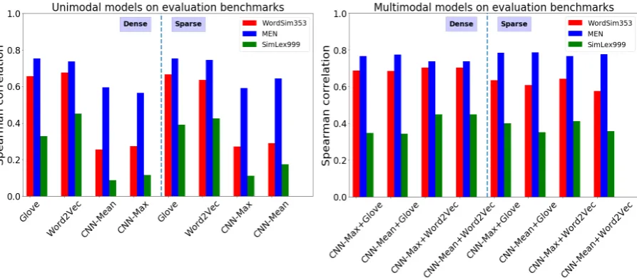
Figure 1: Results for the dense and sparse embeddings for the three semantic similarity benchmarks, for the eight unimodal models (left panel) and the eight multimodal image+text models (right panel).

sparsity parameterλwas set to0.025. Though all sparse embedding matrices are calculated over a smaller lexicon and have a much smaller ding size compared to the original dense embed-dings, in the next section, we investigate how these models still produce competitive results on seman-tic evaluation benchmarks, including neurocogni-tive data.

5 Experiments

The aim of our experiments is to compare the qual-ity of the dense and sparse unimodal and multi-modal embedding models, with a focus on their ability to explain human-derived semantic data. We use several qualitatively different analyses of how well the models explain human-derived mea-sures of semantic representation and processing. In the results that follow, we first demonstrate that sparse multimodal models are competitive with larger dense embedding models on standard se-mantic similarity evaluation benchmarks. We then investigate whether the underlying representations of the sparse, multimodal models are more easily interpreted in terms of human semantic property knowledge about familiar concepts, by evaluating the models’ ability to predict predicates describ-ing property knowledge found in human property norm data. Finally, we evaluate the models’ ability to predict human brain activation data.

5.1 Semantic similarity benchmarks

A widely used evaluation technique for distribu-tional models is the comparison with human

se-mantic similarity rating benchmarks. We evaluate our models on three popular datasets which each reflect slightly different intuitions about semantic similarity.

WordSim353(Finkelstein et al.,2001) consists of353 word pairs with human ratings indicating how related the two concepts in each pair are. The definition of similarity is left quite ambiguous for the human annotators, and words which share any kind of association tend to receive high scores.

MEN(Bruni et al.,2012) consists of3000word pairs with human ratings of how semantically re-lated each pair of concepts are. Pairs with high scores tend to be linked more by semantic relat-edness than by similarity; for example, the words “coffee” and “cup” are semantically related (even though a cup is not similar to coffee). Seman-tic relatedness often corresponds to meronym or holonym concept pairings (e.g. “finger” - “hand”).

SimLex999. (Hill et al., 2015) is a compre-hensive and modern benchmark consisting of999

pairs of words with human ratings of semantic similarity. Semantic similarity tends to reflect words with shared hypernym relations between concept pairs (e.g. “coffee” & “tea” are more sim-ilar than “coffee” & “cup”).

mod-Model Encyclo-pedic

Functional Taxonomic Visual Other Perceptual Overall

CNN-Mean 23.479 28.309 45.756 31.256 26.467 29.244

CNN-Max 22.878 28.765 50.140 32.843 27.508 30.202

GloVe 30.870 37.176 61.517 35.909 38.385 36.984

Word2Vec 27.494 30.372 55.455 32.298 32.800 32.363

GloVe NNSE 31.171 34.645 59.497 35.066 36.738 35.880

Word2Vec NNSE 29.662 34.320 55.073 35.302 33.261 34.956

CNN-Max NNSE 15.320 17.138 26.263 19.646 17.453 18.279

CNN-Mean NNSE 15.996 18.297 27.330 20.954 18.376 19.339

CNN-Max + GloVe 30.669 37.404 63.887 35.790 36.077 36.760

CNN-Mean + GloVe 31.560 38.441 64.459 36.675 36.625 37.637

CNN-Max + Word2Vec 22.114 24.653 51.471 27.566 27.332 27.088

CNN-Mean + Word2Vec 22.057 24.780 51.926 27.527 27.407 27.124

CNN-Max + GloVe JNNSE 32.481 38.787 63.669 39.848 36.245 39.080

CNN-Mean + GloVe JNNSE 31.104 38.009 64.866 40.267 35.998 38.784

CNN-Max + Word2Vec JNNSE 32.718 38.601 61.493 39.663 36.496 38.901

CNN-Mean + Word2Vec JNNSE 31.084 36.939 57.659 38.145 33.436 37.057

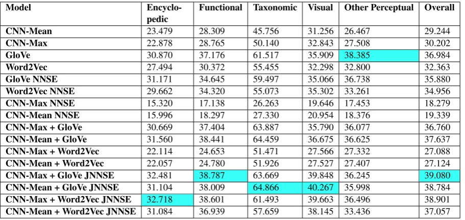
Table 2: Average cross-validation F1×100scores for each model. The blue highlighting indicates the model that scores the highest on each property class.

els, although the overlap is quite high2. Evalua-tions in the next section are based on the subsets of word-pairs for which we have embedding vec-tors for each word.

5.2 Semantic Similarity Results

Figure 1 shows the results for all 16 models on the three evaluation datasets. Even with their sig-nificant dimensionality reduction and forced spar-sity regularisation, the sparse (NNSE) unimodal text and image-based models perform compara-tively with their original dense counterparts, with better results for the sparse unimodal models on several of the benchmarks. The JNNSE mod-els perform comparably to their dense counter-parts, with performance on MEN slightly im-proved, performance on WordSem353 marginally worse, and performance on SimLex999 approxi-mately the same (in spite of the JNNSE models having less than 1/35 times the number dimen-sions of their sparse counterparts)3. Finally, the combined text+image multimodal embeddings are better than unimodal models overall at fitting the similarity rating data. The results on these

con-2_{Atleast 83% for SimLex999, 81% WordSim353 and}

94%for MEN.

3

In order to ensure that the dense models were not disad-vantaged by having more dimensions, we also trained dense text models with200dimensions and found that these did not perform better than the1000-dimensional models. Fur-thermore, we applied SVD to each of the1000-dimensional dense models to reduce the number of dimensions to200but again found the results to be worse than the results for both the1000-dimensional dense models and the sparse models.

ventional benchmarks suggest redundancy in the dense embedding representations, with the sparse embeddings providing a parsimonious representa-tion of semantics that retains informarepresenta-tion about se-mantic similarity. Moreover, multimodal models combining both linguistic and perceptual experi-ence better account for human similarity judge-ments.

5.3 Property norm prediction

Following Collell and Moens (2016) and Lucy and Gauthier(2017), we make use of a dataset of human-derived property norms for a set of con-cepts and analyse how well our distributional mod-els can predict human-elicited property knowledge for words. We use the CSLB property norms ( De-vereux et al.(2014)), a dataset of semantic features for a set of541noun concepts, elicited by partici-pants in a large-scale property norming study. (For example, for “apple”, properties includeis-a-fruit, is-red, grows-on-trees, has-seeds, is-round, etc.). For each embedding model, we train anL2 regu-larised logistic regression classifier for each prop-erty that predicts whether the propprop-erty is true for a given concept.

than five concepts (across the set of concepts ap-pearing in both the CSLB norms and our embed-ding models) were removed, to ensure sufficient positive and negative training cases across con-cepts. To evaluate the logistic regression models’ ability to predict human property knowledge for held-out concepts, we used5-fold cross-validation with stratified sampling to ensure that at least one positive case occurred in each test set. Using the embedding dimensions as training data, we train on the4folds and test on the final fold, and eval-uate the logistic regression classifier by taking the average F1 score over all the test folds. For subse-quent analysis of the fitted regression models for each property, the semantic properties were parti-tioned into the five general classes given in Dev-ereux et al. (2014). These property classes were visual (e.g. is-green; is-round), functional (e.g. is-eaten; used-for-cutting), taxonomic (e.g. is-a-fruit;is-a-tool), encyclopedic (has-vitimans; uses-fuel), andother-perceptual(e.g. is-tasty;is-loud). We hypothesised that properties of different types would differ in how accurately they could be pre-dicted from the different embedding models, given the different sources of information available in the models (for example, visual properties may be more predictable from models trained with image data; see alsoCollell and Moens(2016)).

Table 2 shows the average F1 scores over-all properties and over each of the five property categories. Since the dense and sparse models trained on the same source data (text, images, or text+images) encode similar information, they perform similarly on the task of predicting human semantic property knowledge. However, sparse multimodal models (the last four rows of the ta-ble) are the top scoring models for four of the five property categories, and over the full set of proper-ties (last column of Table2) the top three models are all sparse and multimodal. These results in-dicate that sparse multimodal embeddings are su-perior to their single modality and dense counter-parts in their ability to predict interpretable seman-tic properties corresponding to elements of human conceptual knowledge.

5.4 Interpretating embedding dimensions in terms of semantic properties

Information about a specific semantic property can be stored latently over the dimensions of a seman-tic embedding model, such that the semanseman-tic

prop-erty can be reliably decoded given an embedding vector, as tested in the previous section. However, a stronger test of how closely an embedding model relates to human-elicited conceptual knowledge is to investigate whether the embedding dimensions encode interpretable, human-like semantic prop-erties directly. In other words, does an embedding model learn a set of basis vectors for the semantic space that corresponds to verbalisable, human se-mantic properties like is-round,is-a-fruit, and so on? To address this question, we evaluated how the dense and sparse embeddings differ in their degree of correspondence to the property norms by analysing the fitted parameters of our property prediction logistic regression classifiers. For each embedding model and semantic property, we aver-age the fitted parameters in the logistic regression models across cross-validation iterations and ex-tract the 20 parameters with the highest average magnitude. For each property, we store these20

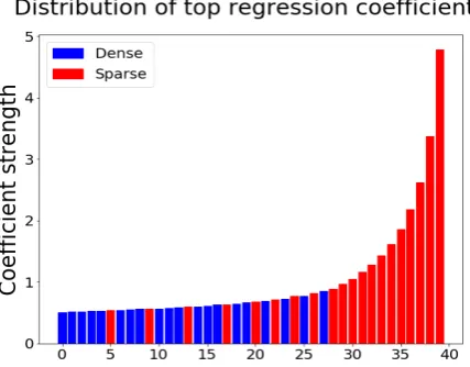
parameters in a vector sorted by decreasing mag-nitude. If a particular semantic property is decod-able directly from only one (or very few) embed-ding dimensions, then the magnitude of the first element (or few elements) of the sorted parameter vector will be very high. Over all properties, we then apply element-wise averaging of the sorted parameter vectors. Figure2shows the magnitudes of these 20 averaged parameters for the dense and sparse multimodal GloVe+CNN-Mean mod-els4. As we can see, the dense model has a more uniform distribution, indicating that the informa-tion is highly diffuse over the dimensions of the dense embedding space. Conversely, the top few parameters for the sparse model have very high magnitude, indicating that, on average, informa-tion about semantic properties tend to be strongly associated with a small number of dimensions in the sparse space.

As a further test of how well dimensions of embedding models correspond to human semantic knowledge, we calculated pairwise correlations, across concepts, between embedding dimensions and properties. For a given semantic property, we can test which of two embedding models best en-code that semantic property in a single dimension – an embedding model that more directly matches the property norm data will tend to have a di-mension that correlates more strongly with that

4_{The results are similar for all other pairs of sparse and}

GloVe Word2Vec CNN-Max CNN-Mean CNN-Max + GloVe

CNN-Mean + GloVe

CNN-Max + Word2Vec

CNN-Mean + Word2Vec

fMRI (S) 0.654 0.652 0.641 0.647 0.662 0.686 0.649 0.671

fMRI (D) 0.670 0.676 0.654 0.651 0.673 0.677 0.676 0.676

MEG (S) 0.664 0.669 0.651 0.641 0.671 0.668 0.675 0.665

MEG (D) 0.680 0.664 0.654 0.643 0.684 0.684 0.664 0.664

Table 3: Results of all sparse (S) and dense (D) models on 2 vs. 2 tests against the fMRI and MEG neuroimaging data, averaged over participants.

Figure 2: The ranking of the top20model coeffi-cients for the logistic regression classifiers trained on each feature, for the dense GloVe + CNN-Mean model (blue bars), and the joint sparse GloVe + CNN-Mean model (red bars).

property than anydimension of a model that en-codes information about that property more la-tently. For this analysis, we first filtered the set of concepts in the dense models to include only the concepts in the CSLB norms, and recalculated the (J)NNSE sparse models over these concepts only. We tuned the sparsity parameter so that the sparsity of the sparse embedding models closely matched the sparsity of CSLB concept-property matrix (97% sparse), and kept the dimensionality of the sparse embeddings the same as our original sparse models. LetvP be the values for a property

Pfor each concept in the CSLB norms, and letMd

and Ms represent the set of embedding columns

for a dense model and its sparse counterpart re-spectively. Then for each propertyP, we evaluate the inequality

maxc∈Md(ρ(c, vP))< maxc∈Ms(ρ(c, vP))

whereρis the Spearman correlation. We count the proportion of times the inequality is true across all properties in the norms, repeat this for each of the eight dense models and their sparse counterparts,

and calculate the average. The results show that the sparse models have the most correlated dimen-sion63.2%of the time. In order to ensure that the dense models were not disadvantaged by having more dimensions (and to test that the sparsity con-straint rather than dimensionality reduction was the reason for the superior performance of the sparse models), we used SVD on all dense models to reduce the dimensions down to the same size as their sparse counterparts and reran the test. Here the results show that the sparse models have the most correlated dimension81.1%of the time, in-dicating that the sparse models do learn semantics-encoding dimensions from the dense models that more closely correspond to human-derived prop-erty knowledge.

5.5 Evaluation on brain data

For our final set of analysis, we tested how closely each of the eight dense and eight sparse models relate to neurocognitive processing in the human brain. We used BrainBench (Xu et al.,2016), an evaluation benchmark for semantic models that al-lows us to evaluate each model’s ability to predict patterns of activation in neuroimaging data. The BrainBench dataset includes brain activation data recorded using two complementary neuroimaging modalities:fMRI(which measures cerebral blood oxygenation and which has relatively good spa-tial resolution but poor temporal resolution) and MEG (which measures aggregate magnetic field changes induced by neural activity and which has good temporal resolution but poorer spatial reso-lution). The neuroimaging data in both modalities are taken from nine participants that viewed pic-tures of60different concepts.

GloVe Word2Vec CNN-Max CNN-Mean CNN-Max + GloVe

CNN-Mean + GloVe

CNN-Max + Word2Vec

CNN-Mean + Word2Vec

fMRI (D) 0.162 0.164 0.145 0.151 0.150 0.152 0.152 0.155

fMRI (S) 0.138 0.136 0.140 0.144 0.139 0.140 0.154 0.168

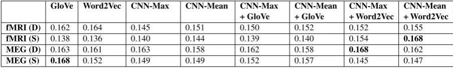
MEG (D) 0.163 0.161 0.163 0.158 0.162 0.158 0.168 0.162

MEG (S) 0.168 0.152 0.149 0.149 0.152 0.157 0.145 0.147

Table 4: Average RSA results (Spearman’sρ) for all sparse (S) and dense (D) models.

similarity matrix M where each element Mi,j in

the matrix is the correlation between the embed-ding vectors of the distributional model for the i-th andj-th concepts. In Brainbench, the brain data is already preprocessed and transformed into such a representation for both the fMRI and MEG neu-roimaging modalities, giving a 60 ×60 similar-ity matrix for each participant for both modalities. The next step for BrainBench evaluation is to per-form a “2 vs.2” test between each distributional model and the brain data. LetMD andMBbe the

similarity matrices associated with a distributional semantic model and a participant’s brain data re-spectively. Letrbe the Pearson correlation func-tion, then a 2vs. 2test is a positive case for any two pairs of conceptsw1andw2if

r(MD(w1), MB(w1)) +r(MD(w2), MB(w2)) > r(MD(w1), MB(w2)) +r(MD(w2), MB(w1))

where MD(w1) and MD(w2) denote the rows of values corresponding to the concepts w1 and w2 respectively, omitting the columns that cor-respond to the correlation between w1 and w2. This 2 vs. 2 test is performed on all pairs of the 60 concepts, to obtain the proportion of pos-itive cases for the pair MD and MB. The

dis-tributional models are evaluated against all brain-based representations and averaged by imaging modality. The results for both sparse and dense models are displayed in Table 3. For the fMRI data, the model with the highest average 2 vs.2

test score is the sparse multimodal GloVe+CNN-Max embedding, whilst on the MEG data the highest scoring model is a tie between the dense multimodal GloVe+CNN-Max embedding and the dense multimodal GloVe+CNN-Mean embedding. The results demonstrate that semantic distribu-tional models that encode a range of different in-formation are better at making statistically signifi-cant predictions on brain data. In general, the mul-timodal models do better than the unimodal text and image models at fitting the brain data.

Finally, we computed the direct correlation

be-tween the representationsMD andMB, using the

technique of Representational Semantic Analsy-sis (RSA) (Kriegeskorte et al., 2008) commonly employed in cognitive neuroscience. Given that MD andMB have the same number of words and

word indexing (words associated with certain rows and columns are shared across representations), we take the Spearman’s correlation between the flattened upper triangular similarity matrices of these two representations for each pair of DSM and brain dataset5.

For a given distributional model, we average all Spearman correlation values across the nine par-ticipants for each imaging modality; the results are presented in Table 4. The results show that sparse models give the closest representation to both fMRI and MEG data, with the multimodal sparse word2vec+CNN-Mean model best fitting the fMRI data, and the sparse GloVe model best fitting the MEG data. These results indicate that semantic model sparsity is an important property reflected in neurocognitive semantic representa-tions.

6 Conclusion

In this paper, we have demonstrated the repre-sentational potential of sparse multimodal distri-butional models using several qualitatively dif-ferent and complimentary evaluation tasks that are derived from human data: semantic similar-ity ratings, conceptual property knowledge, and neuroimaging data. We show that both sparse and multimodal embeddings achieve a more faith-ful representation of human semantics than dense models constructed from a single information source.

5

Usually RSA is performed on a new matrix produced by subtracting anN ×N matrix of all1’s from these concept matricesMD and MB, where N is the number of shared

concepts. Such a representation is known as a Representa-tional Dissimilarity Matrix(RDM), although here we follow

7 Acknowledgements

We would like to thank Partha Talukdar for gen-erously providing us with the code for the Non-Negative Sparse Embedding algorithm. We would also like to thank Alona Fyshe for providing the Joint Non-Negative Sparse Embedding code.

References

Stanislaw Antol, Aishwarya Agrawal, Jiasen Lu, Mar-garet Mitchell, Dhruv Batra, C Lawrence Zitnick, and Devi Parikh. 2015. Vqa: Visual question an-swering. InProceedings of the IEEE International Conference on Computer Vision, pages 2425–2433. Miroslav Batchkarov, Thomas Kober, Jeremy Reffin,

Julie Weeds, and David Weir. 2016. A critique of word similarity as a method for evaluating distribu-tional semantic models.

Elia Bruni, Gemma Boleda, Marco Baroni, and Nam-Khanh Tran. 2012. Distributional semantics in tech-nicolor. In Proceedings of the 50th Annual Meet-ing of the Association for Computational LMeet-inguis- Linguis-tics: Long Papers-Volume 1, pages 136–145. Asso-ciation for Computational Linguistics.

Elia Bruni, Nam-Khanh Tran, and Marco Baroni. 2014. Multimodal distributional semantics. Journal of Ar-tificial Intelligence Research, 49:1–47.

Alex Clarke, Barry J. Devereux, Billi Randall, and Lor-raine K. Tyler. 2015. Predicting the time course of individual objects with meg. Cerebral Cortex, 25(10):3602–3612.

Guillem Collell and Marie-Francine Moens. 2016. Is an image worth more than a thousand words? on the fine-grain semantic differences between visual and linguistic representations. In Proceedings of COL-ING 2016, the 26th International Conference on Computational Linguistics: Technical Papers, pages 2807–2817. The COLING 2016 Organizing Com-mittee.

Guillem Collell, Ted Zhang, and Marie-Francine Moens. 2017. Imagined visual representations as multimodal embeddings. In AAAI, pages 4378– 4384.

Jia Deng, Wei Dong, Richard Socher, Li-Jia Li, Kai Li, and Li Fei-Fei. 2009. Imagenet: A large-scale hi-erarchical image database. InComputer Vision and Pattern Recognition, 2009. CVPR 2009. IEEE Con-ference on, pages 248–255. IEEE.

Barry Devereux, Colin Kelly, and Anna Korhonen. 2010. Using fmri activation to conceptual stim-uli to evaluate methods for extracting conceptual representations from corpora. In Proceedings of the NAACL HLT 2010 First Workshop on Compu-tational Neurolinguistics, pages 70–78. Association for Computational Linguistics.

Barry J Devereux, Alex Clarke, Andreas Marouchos, and Lorraine K Tyler. 2013. Representational sim-ilarity analysis reveals commonalities and differ-ences in the semantic processing of words and objects. Journal of Neuroscience, 33(48):18906– 18916.

Barry J Devereux, Alex Clarke, and Lorraine K Tyler. 2018. Integrated deep visual and semantic attrac-tor neural networks predict fmri pattern-information along the ventral object processing pathway. Scien-tific Reports, 8:10636.

Barry J Devereux, Lorraine K Tyler, Jeroen Geertzen, and Billi Randall. 2014. The centre for speech, lan-guage and the brain (cslb) concept property norms. Behavior research methods, 46(4):1119–1127. Manaal Faruqui, Yulia Tsvetkov, Dani Yogatama, Chris

Dyer, and Noah Smith. 2015. Sparse overcom-plete word vector representations. arXiv preprint arXiv:1506.02004.

Lev Finkelstein, Evgeniy Gabrilovich, Yossi Matias, Ehud Rivlin, Zach Solan, Gadi Wolfman, and Ey-tan Ruppin. 2001. Placing search in context: The concept revisited. InProceedings of the 10th inter-national conference on World Wide Web, pages 406– 414. ACM.

Alona Fyshe, Partha P Talukdar, Brian Murphy, and Tom M Mitchell. 2014. Interpretable semantic vec-tors from a joint model of brain-and text-based meaning. In Proceedings of the conference. Asso-ciation for Computational Linguistics. Meeting, vol-ume 2014, page 489. NIH Public Access.

Anna Gladkova and Aleksandr Drozd. 2016. Intrinsic evaluations of word embeddings: What can we do better? InRepEval@ACL.

James V Haxby, M Ida Gobbini, Maura L Furey, Alu-mit Ishai, Jennifer L Schouten, and Pietro Pietrini. 2001. Distributed and overlapping representations of faces and objects in ventral temporal cortex. Sci-ence, 293(5539):2425–2430.

Felix Hill, Roi Reichart, and Anna Korhonen. 2015. Simlex-999: Evaluating semantic models with (gen-uine) similarity estimation. Computational Linguis-tics, 41(4):665–695.

Patrik O Hoyer. 2002. Non-negative sparse coding. In Neural Networks for Signal Processing, 2002. Pro-ceedings of the 2002 12th IEEE Workshop on, pages 557–565. IEEE.

Alexander G Huth, Wendy A de Heer, Thomas L Grif-fiths, Fr´ed´eric E Theunissen, and Jack L Gallant. 2016. Natural speech reveals the semantic maps that tile human cerebral cortex. Nature, 532(7600):453– 458.

on computer vision and pattern recognition, pages 3128–3137.

Douwe Kiela and L´eon Bottou. 2014. Learning image embeddings using convolutional neural networks for improved multi-modal semantics. InProceedings of the 2014 Conference on Empirical Methods in Nat-ural Language Processing (EMNLP), pages 36–45. Nikolaus Kriegeskorte, Marieke Mur, and Peter A

Ban-dettini. 2008. Representational similarity analysis-connecting the branches of systems neuroscience. Frontiers in systems neuroscience, 2:4.

Alex Krizhevsky, Ilya Sutskever, and Geoffrey E Hin-ton. 2012. Imagenet classification with deep con-volutional neural networks. In Advances in neural information processing systems, pages 1097–1105. Angeliki Lazaridou, Nghia The Pham, and Marco

Ba-roni. 2015. Combining language and vision with a multimodal skip-gram model. arXiv preprint arXiv:1501.02598.

Li Lucy and Jon Gauthier. 2017. Are distributional representations ready for the real world? evaluat-ing word vectors for grounded perceptual meanevaluat-ing. arXiv preprint arXiv:1705.11168.

Julien Mairal, Francis Bach, Jean Ponce, and Guillermo Sapiro. 2010. Online learning for matrix factorization and sparse coding. Journal of Machine Learning Research, 11(Jan):19–60.

Ken McRae, George S Cree, Mark S Seidenberg, and Chris McNorgan. 2005. Semantic feature produc-tion norms for a large set of living and nonliving things. Behavior research methods, 37(4):547–559. Tomas Mikolov, Ilya Sutskever, Kai Chen, Greg S Cor-rado, and Jeff Dean. 2013. Distributed representa-tions of words and phrases and their compositional-ity. InAdvances in neural information processing systems, pages 3111–3119.

George A Miller. 1995. Wordnet: a lexical database for english. Communications of the ACM, 38(11):39– 41.

Tom M Mitchell, Svetlana V Shinkareva, Andrew Carl-son, Kai-Min Chang, Vicente L Malave, Robert A Mason, and Marcel Adam Just. 2008. Predicting human brain activity associated with the meanings of nouns.science, 320(5880):1191–1195.

Brian Murphy, Partha Talukdar, and Tom Mitchell. 2012. Learning effective and interpretable semantic models using non-negative sparse embedding. Pro-ceedings of COLING 2012, pages 1933–1950. Jiquan Ngiam, Aditya Khosla, Mingyu Kim, Juhan

Nam, Honglak Lee, and Andrew Y Ng. 2011. Multi-modal deep learning. InProceedings of the 28th in-ternational conference on machine learning (ICML-11), pages 689–696.

Maxime Oquab, Leon Bottou, Ivan Laptev, and Josef Sivic. 2014. Learning and transferring mid-level im-age representations using convolutional neural net-works. InComputer Vision and Pattern Recognition (CVPR), 2014 IEEE Conference on, pages 1717– 1724. IEEE.

Jeffrey Pennington, Richard Socher, and Christopher Manning. 2014. Glove: Global vectors for word representation. InProceedings of the 2014 confer-ence on empirical methods in natural language pro-cessing (EMNLP), pages 1532–1543.

Lutfi Kerem Senel, Ihsan Utlu, Veysel Yucesoy, Aykut Koc, and Tolga Cukur. 2017. Semantic structure and interpretability of word embeddings. arXiv preprint arXiv:1711.00331.

Carina Silberer, Vittorio Ferrari, and Mirella Lapata. 2017. Visually grounded meaning representations. IEEE transactions on pattern analysis and machine intelligence, 39(11):2284–2297.

Anders Søgaard. 2016. Evaluating word embeddings with fmri and eye-tracking. In Proceedings of the 1st Workshop on Evaluating Vector-Space Represen-tations for NLP, pages 116–121.

Luis Von Ahn and Laura Dabbish. 2004. Labeling im-ages with a computer game. InProceedings of the SIGCHI conference on Human factors in computing systems, pages 319–326. ACM.

Haoyan Xu, Brian Murphy, and Alona Fyshe. 2016. Brainbench: A brain-image test suite for distribu-tional semantic models. InProceedings of the 2016 Conference on Empirical Methods in Natural Lan-guage Processing, pages 2017–2021.