A STUDY ON THE BEHAVIOUR OF VOLATILITY OF THE INDIAN COMMODITY MARKET
1
Ranajit Chakraborty
1
Department of Business Management, University of Calcutta, 1, Reformatory Street, Kolkata
2
Department of Basic Science, Techno India College of Technology, New Town, Rajarhat, Kolkata: 700156
ARTICLE INFO ABSTRACT
The objective of this study was to examine the behaviour of volatility in the Indian commodity market after the introduction of derivative trading in the national level commodity exchanges. Researchers around the world revealed the behaviour of volatility
them studied the Indian commodity market extensively in this aspect. From 2004 to 2012, this 9 year period was chosen as the period of study. The agricultural commodity index MCXAGRI, some of the agricultural com
some non
of volatility. Using entropy as a measure of volatility, it was observed that
commodities spot and futures prices volatility behave in a similar manner. However, there were exceptions for some commodities. No trend of volatility was observed for most of the commodities in Indian market. Additionally, with few excepti
and futures prices was insignificant. Furthermore, patterns of change of volatility over the quarters was similar in the spot and the futures markets.
Copyright © 2015 Ranajit Chakraborty and Rahuldeb Das
permits unrestricted use, distribution, and reproduction in any medium, provided the original work is properly cited.
INTRODUCTION
Volatility has always been a matter of great concern to the market participants, especially, for commodities, producers, merchandisers and traders— all being affected by the volatility of the market. The random fluctuations of the commodity prices are termed as volatility. It also can be considered as the uncertainty associated with the commodity prices. Sometimes movements of the stock or commodity markets cannot be justified by the changes in the fundamentals of the markets. Then volatility of the market requires special attention of the traders and financial experts. According to the efficient market hypothesis, information affects the prices. Therefore, volatility is said to be the result of the information provided to the market. It changes according to the arrival of new information in the market. Another school of thought in this regard describes volatility as a result of the behavioural activity of the investors. The reactions of the investors, due to their psychological and social belief, have a stro
market. Any significant drop in the market causes volatility. Traders overreact to the market condition in this period, since market drops are associated with increased uncertainty regarding the future market conditions and recovery time.
Corresponding author: Rahuldeb Das
Department of Basic Science, Techno India College of Technology, New Town, Rajarhat, Kolkata: 700156
ISSN: 0975-833X
Article History: Received 16th June, 2015 Received in revised form 24th July, 2015
Accepted 23rd August, 2015
Published online 16th September,2015
Citation: Ranajit Chakraborty and Rahuldeb Das, International Journal of Current Research, 7, (9), Key words: Commodity Market, Entropy, Volatility, Trend.
RESEARCH ARTICLE
A STUDY ON THE BEHAVIOUR OF VOLATILITY OF THE INDIAN COMMODITY MARKET
Ranajit Chakraborty and *
,2Rahuldeb Das
Department of Business Management, University of Calcutta, 1, Reformatory Street, Kolkata
Department of Basic Science, Techno India College of Technology, New Town, Rajarhat, Kolkata: 700156
ABSTRACT
The objective of this study was to examine the behaviour of volatility in the Indian commodity market after the introduction of derivative trading in the national level commodity exchanges. Researchers around the world revealed the behaviour of volatility in different commodity markets, but none of them studied the Indian commodity market extensively in this aspect. From 2004 to 2012, this 9 year period was chosen as the period of study. The agricultural commodity index MCXAGRI, some of the agricultural commodities, namely Barley, Chickpea, Chilli, Cumin, Maize, Mustard Seed, Pepper and some non-agricultural commodities namely Brent Crude Oil and Gold were involved in the analysis of volatility. Using entropy as a measure of volatility, it was observed that
commodities spot and futures prices volatility behave in a similar manner. However, there were exceptions for some commodities. No trend of volatility was observed for most of the commodities in Indian market. Additionally, with few exceptions, the difference between average volatility of the spot and futures prices was insignificant. Furthermore, patterns of change of volatility over the quarters was similar in the spot and the futures markets.
uldeb Das. This is an open access article distributed under the Creative Commons Attribution License, which permits unrestricted use, distribution, and reproduction in any medium, provided the original work is properly cited.
Volatility has always been a matter of great concern to the market participants, especially, for commodities, producers, all being affected by the volatility of the market. The random fluctuations of the commodity ed as volatility. It also can be considered as the uncertainty associated with the commodity prices. Sometimes movements of the stock or commodity markets cannot be justified by the changes in the fundamentals of the markets. requires special attention of the traders and financial experts. According to the efficient market hypothesis, information affects the prices. Therefore, volatility is said to be the result of the information provided to the the arrival of new information in the market. Another school of thought in this regard describes volatility as a result of the behavioural activity of the investors. The reactions of the investors, due to their psychological and social belief, have a strong impact on the market. Any significant drop in the market causes volatility. Traders overreact to the market condition in this period, since market drops are associated with increased uncertainty regarding the future market conditions and recovery time.
Department of Basic Science, Techno India College of Technology,
A tendency of excessive buying or selling is observed due to the fear of future market condition, and these activi
the volatility of the market. This volatility keeps on changing over time, according to the arrival of information about a financial security or a commodity. So the market has to go through alternate periods of high volatility and low volatili The high volatility period does not stay longer; the market absorbs the shock with time. However, volatility should not always be treated as an indication of a bad market condition; on the other hand, contributes to the efficient price innovation of a market.
The main objective of this paper is to study the behaviour of volatility in the Indian commodity market. By examining spot and futures market for commodities, this study intends to reveal whether both markets behave in a similar manner. Volatility is one of the important aspects which have to be studied in order to understand the behaviour of the commodity market. In finance, a number of researchers have used variance or standard deviation as measures of uncertainty. However, according to Soofi (1997), these measures may fail in some specific situations, since they require the underlying probability distribution to be symmetric. Furthermore, they neglect the possibility of extreme events such as the existence of fat-tails. Because of this fact,
been used in this paper to estimate volatility. Entropy involves
Available online at http://www.journalcra.com
International Journal of Current Research Vol. 7, Issue, 09, pp.20296-20307, September, 2015
INTERNATIONAL
Rahuldeb Das, 2015. “A study on the behaviour of volatility of the indian commodity market”, , 7, (9),20296-20307.
z
A STUDY ON THE BEHAVIOUR OF VOLATILITY OF THE INDIAN COMMODITY MARKET
Department of Business Management, University of Calcutta, 1, Reformatory Street, Kolkata – 700027
Department of Basic Science, Techno India College of Technology, New Town, Rajarhat, Kolkata: 700156
The objective of this study was to examine the behaviour of volatility in the Indian commodity market after the introduction of derivative trading in the national level commodity exchanges. Researchers in different commodity markets, but none of them studied the Indian commodity market extensively in this aspect. From 2004 to 2012, this 9 year period was chosen as the period of study. The agricultural commodity index MCXAGRI, some of the modities, namely Barley, Chickpea, Chilli, Cumin, Maize, Mustard Seed, Pepper and agricultural commodities namely Brent Crude Oil and Gold were involved in the analysis of volatility. Using entropy as a measure of volatility, it was observed that for most of the commodities spot and futures prices volatility behave in a similar manner. However, there were exceptions for some commodities. No trend of volatility was observed for most of the commodities in ons, the difference between average volatility of the spot and futures prices was insignificant. Furthermore, patterns of change of volatility over the quarters
This is an open access article distributed under the Creative Commons Attribution License, which
A tendency of excessive buying or selling is observed due to the fear of future market condition, and these activities trigger the volatility of the market. This volatility keeps on changing over time, according to the arrival of information about a financial security or a commodity. So the market has to go through alternate periods of high volatility and low volatility. The high volatility period does not stay longer; the market absorbs the shock with time. However, volatility should not always be treated as an indication of a bad market condition; on the other hand, contributes to the efficient price innovation
The main objective of this paper is to study the behaviour of volatility in the Indian commodity market. By examining spot and futures market for commodities, this study intends to reveal whether both markets behave in a similar manner. y is one of the important aspects which have to be studied in order to understand the behaviour of the commodity market. In finance, a number of researchers have used variance or standard deviation as measures of uncertainty. However, 997), these measures may fail in some specific situations, since they require the underlying probability distribution to be symmetric. Furthermore, they neglect the possibility of extreme events such as the existence tails. Because of this fact, a new measure entropy has been used in this paper to estimate volatility. Entropy involves
INTERNATIONAL JOURNAL OF CURRENT RESEARCH
higher order moments of a distribution and uses more information about the underlying probability distribution of a data than the variance. So, entropy will provide a very good estimate of volatility for the commodity markets. In addition, a comparison between the volatility of the spot and futures market for commodities has been drawn. Since spot and futures prices express the value of the same underlying commodity, they are supposed to move together. Therefore, the patterns of behaviour of volatility in both the markets should be similar. In this regard, trend of volatility has been checked in both the markets at the outset. Also, two-sample-mean-test has been performed to examine whether both spot and futures markets have similar average volatility; both parametric and non-parametric methods have been used in this purpose. The pattern of the change of volatility is another matter of concern while judging the overall volatility behaviour of a market. Two sample variance tests have been used to examine the change of volatility over the quarters. After the introduction of derivative trading in the Indian commodity market, this is the first study in Indian commodity market with a focus on the behaviour of volatility of the market. Finally, it is also to be noted here that use of entropy to estimate volatility is relatively new in the context of Indian market.
Literature Review
Very few literatures in finance have studied the behaviour of volatility of the commodity market. Specially, use of entropy as a measure of uncertainty is relatively new in financial domain. Haugen et al. (1991) have estimated the volatility changes in daily returns to the Dow Jones Industrial Average. They have tested the change of stock prices and their expected returns due to the change of volatility. Evidence of relatively large and systematic revisions in stock prices and subsequent expected returns was found. They have also concluded that the majority of the volatility changes cannot be associated with the release of significant economic information. Giot (2003) examined the incremental information content of lagged implied volatility to skewed student GARCH models for a collection of agricultural commodity cocoa, coffee, and sugar traded on the New York Board of Trade. He has found that the implied volatility for option on future contracts has a high information content regarding conditional variance and VaR forecasts of the underlying future forecasts. Bandivadekar and Ghosh (2003) have studied the impact of introduction of index futures on the spot market volatility on both S&P CNX Nifty and BSE Sensex using ARCH/GARCH technique.
They have concluded that due to the increased impact of recent news and reduced effects of uncertainty originating from the old news, the spot market volatility is decreased after the introduction of index futures. They also observed that the market wide volatility has fallen during the period under their consideration. Their analysis shows that the futures effect plays a definite role in the reduction of volatility in the case of S&P CNX Nifty. Pindyck (2004) examined the role of volatility in the short-run commodity market dynamics and the determinants of volatility. He developed a structural model of inventories, spot, and futures prices that explicitly accounts for volatility. He estimated it using daily and weekly data for the
petroleum complex: crude oil, heating oil, and gasoline. He found that changes in volatility influence market variables, but the effects are not large. He concluded that changes in volatility can help explain the changes in the spot-futures spread, but not the changes in the spot price itself. Raju and Ghosh (2004) have compared the Indian market with some of the international markets in respect of volatility. They observed that India provides as high a return as the US and the UK market could provide but the volatility is higher. Comparatively, Indian market shows less of skewness and kurtosis. They also added that intra-day volatility in Indian market is also very much under control and has come down compared to past years. Dionísio et al. (2005) have described entropy as a more general measure of certainty than the variance, since it uses much more information about the probability distribution. They also have found that mutual information and conditional entropy can be used for estimating systematic risk and specific risk. Pal (2005) concluded that Foreign Institutional Investors (FII) have a strong influence on the volatility of the Indian stock market. Moreover, FIIs has a strong hold on the companies that constitutes the Sensex. Adrian and Rosenberg (2008) have examined the cross-sectional pricing of volatility risk by decomposing equity market volatility into short-run and long-run components. They observed that risk of prices is negative and significant for both volatility components. The short-run component captures the market skews risk, which is interpreted as a measure of the tightness of financial constraints. The long-run component represents the business cycle risk.
Data
Data for this study has been collected from the Multi Commodity Exchange (MCX) and the National Commodity Derivative Exchange (NCDEX) of India. The period of study is from 1st January 2004 to 31 December 2012. Spot and futures prices of the agricultural-commodity index MCXAGRI is taken from the MCX website. Daily spot and futures closing price of Barley, Chickpea, Chilli, Cumin, Maize, Mustard Seed, Pepper, Brent Crude Oil and Gold obtained from the website of NCDEX.
Methodology
Daily closing spot and futures prices for the commodities Barley, Chickpea, Chilli, Cumin, Maize, Mustard Seed, Pepper, Brent Crude Oil and Gold and the commodity index MCXAGRI have been used for this study. The returns from the prices of every commodity and commodity index have been calculated using the following formula
Rt = × 100 …………...1
Where, Rt is the return of a commodity at time t, Yt and Yt-1
are the prices of a commodity at time t and t-1 respectively.
Augmented Dickey-Fuller Test (ADF)
Stationarity of all return series have been checked by Augmented Dickey-Fuller (ADF) test. The equation of ADF test is given below:
∆Yt = µ + bt + βYt-1 – ∑ ∆ + єt ………..2
Here Yt is a time series which is to be tested for stationarity,
∆Yt is the first order differenced series based on Yt, i.e., ∆Yt =
Yt - Yt-1, µ is the intercept term, b is the coefficient of a time
trend, β is the coefficient of the lagged value of Yt, , j =
1(1)p, are the coefficient of the autoregressive process of ∆Yt,
and єt is white noise residual. The hypothesis under
consideration is
H0: b = β = 0.
Therefore, an F-test is performed on the hypothesis H0. If β = 0
then there is a unit root. If Unit Root is present in the series, then it is non-stationary.
Volatility of an index is usually calculated by its standard deviation. It is a very well known measure of uncertainty. But, according to Maasoumi (1993), entropy can be an alternative measure of dispersion. The variance measures an average of the distances of outcomes of the probability distribution from the mean. But, the entropy is a measure of disparity of the density pX(x) from the uniform distribution. In this context,
Soofi (1997) has mentioned that the interpretation of the variance as a measure of uncertainty must be done with some precaution. According to Ebrahimi, Maasoumi and Soofi (1999), both variance and entropy reflect concentration, but their metrics for concentration are different. Unlike the variance which measures concentration only around the mean, the entropy measures diffuseness of the density irrespective of the location of concentration. Also entropy depends on many more parameters of a distribution than the variance. Entropy is related to higher order moments of a distribution as a result it, uses much more information about the probability distribution than the variance. Arafat, Skubic and Keegan (2003) suggested that entropy can be treated as a good measure of uncertainty. So, in this chapter entropy has been used as a measure of volatility.
Entropy
If a set of possible events has probabilities of occurrence p1,...,
pn. According to Shannon (1948) the entropy is defined as
H (Y) = − ∑ ……….3
When the random variable has a continuous distribution, and pY(Y) is the density function of the random variable Y, the
entropy is given by
H(Y)= -∫ ( ) ( ) ………4
For a commodity, each return series (spot and futures) has been partitioned into quarterly series. For each quarterly series volatility has been calculated using the concept of entropy.
Mann-Kendall Trend Test
To test the existence of trend in the volatility of the spot and futures prices of the commodities, Mann-Kendall trend test has been used. Given n consecutive observations of a time series Yt, t = 1, · · · , n. Mann (1945) suggested using the Kendall
rank correlation of Yt with t, t = 1, · · · , n to test for monotonic
trend. The null hypothesis of no trend assumes that the Yt, t =
1, · · · , n are independently distributed. The hypotheses under consideration is :
H0 :No monotonic trend is present in Yt .
Against the alternative
H1:Monotonic trend is present in Yt .
In the case of no ties in the values of Yt, t = 1, · · ·n , the
Mann-Kendall rank correlation for a trend test can be written as
T = , ..………5
where
S = 2P − , ………...6
where P is the number of times that > for all t1, t2 = 1, . .
. , n such that t2 > t1. Thus T = 2πc − 1, where πc is the relative
frequency of positive concordance, i.e., the proportion of time for which > when t2 > t1. Equivalently, the relative
frequency of positive concordance is given by πc= 0.5(T + 1).
Shapiro–Wilk Test
The Shapiro–Wilk test is used to check whether a sample Y1,
..., Yn, of spot or futures prices volatility, came from a normally
distributed population. The hypotheses under this test is given by:
H0 : The distribution of the data sample is normal.
Against the alternative
H1 : The distribution of the data sample is non-normal.
The test statistic is:
= (∑ ( ))
∑ ( ) ……….7
where ( ), = 1(1) is the ith order statistic, i.e., the ith
smallest number in the sample; is the sample mean; the constants are given by
( , … , ) =
( )
………..8
where = ( , … , ) and ( , … , ) are the expected
values of the order statistics of independent and identically distributed random variables sampled from the standard normal distribution, and V is the covariance matrix of those order statistics. The null hypothesis will be rejected if is below a predetermined threshold.
Welch's t-Test
To test whether two volatility samples (spot and futures) have equal means when the sample variances are unequal,
Welch's t-test is applied. The hypotheses considered in this test are:
H0 : µ1 = µ2
Against the alternative,
H1 : µ1 ≠ µ2
Where,
µ1 = mean volatility of the 1st population
µ2 = mean volatility of the 2nd population
Welch's t-test defines the statistic t by the following formula:
=
………
where, , and are the sample mean
variance and sample size, respectively for the 1 similar notation is followed for the 2nd sample. The
freedom associated with this variance estimate are
approximated using the Welch–Satterthwaite equation
≈ ( )
Here, = − 1, the degrees of freedom associated with
the 1st variance estimate. = − 1 , the degrees of
freedom associated with the 2nd variance estimate.
Kolmogorov–Smirnov Two Sample Test
The Kolmogorov–Smirnov two sample test
whether the probability distributions of two samples differ.
H0 :F1 = F2
Against the alternative,
H1 :F1 ≠ F2
Where,
F1 = probability distribution of the 1 st
population F2 = probability distribution of the second population
In this case, the Kolmogorov–Smirnov statistic is
. ′= sup | , ( ) − , ′( ) |
where , and , ′ are the empirical distribution
functions of the first and the second sample respectively.
n’ are the sample sizes of the 1st and 2nd sample respect The null hypothesis is rejected at level if
. ′> ( )
′ ′
The value of ( ) is specified for each level of
20299 Ranajit Chakraborty and Rahuldeb Das
test is applied. The hypotheses considered in this test
by the following formula:
………9
sample mean, sample , respectively for the 1st sample. A sample. The degrees of associated with this variance estimate are
Satterthwaite equation:
………10
, the degrees of freedom associated with , the degrees of variance estimate.
is applied to test whether the probability distributions of two samples differ.
population = probability distribution of the second population
Smirnov statistic is
……….11
empirical distribution of the first and the second sample respectively. n and sample respectively.
is specified for each level of .
F-Test
The equality of variance between the spot and futures prices volatility samples is checked by F
samples have to be independent and identically distributed each of them should follow
hypotheses considered in these tests are given by
H0 : σ21 = σ22
Against the alternative,
H1 : σ21 ≠ σ22
Where,
σ21 = variance of the 1st population
σ22 = variance of the 2nd population
The test statistic
=
has F-distribution with − 1
freedom. s and s are the samples variances of the 1 2nd sample having sample sizes
Levene’s Test
For the volatility samples that violate normality assumptions, F-test cannot be applied. In this case a non
Levene’s test, is applied to check the equality of variance between the spot and futures prices volatility samples. hypotheses considered in these tests are given by:
H0 : σ21 = σ22
Against the alternative,
H1 : σ21 ≠ σ22
Where,
σ21 = variance of the 1 st
population σ22 = variance of the 2nd population
The test statistic for this test, W
= ( ) ∑ ( )
( ) ∑ ∑ ( )
where is the number of samples,
observations, is the number of observations in the
, = 1(1) , = 1(1) is the value of volatility for the observation from the ith sample,
= − , ℎ
= − , ℎ
̿ = ∑ ∑ ,
= ∑ .
Ranajit Chakraborty and Rahuldeb Das,A study on the behaviour of volatility of the Indian commodity market
The equality of variance between the spot and futures prices volatility samples is checked by F-test. For this test, the independent and identically distributed and each of them should follow normal distribution. The hypotheses considered in these tests are given by:
population population
.………12
and − 1 degrees of
are the samples variances of the 1st and the
sample having sample sizes and respectively.
For the volatility samples that violate normality assumptions, test cannot be applied. In this case a non-parametric test, Levene’s test, is applied to check the equality of variance between the spot and futures prices volatility samples. The
considered in these tests are given by:
population population
W, is defined as follows:
.………13
is the number of samples, is the total number of is the number of observations in the ith sample, is the value of volatility for the jth sample,
ℎ
ℎ ,
The significance of W is tested against ( , − 1, − ) where F is a quantile of the F distribution, with − 1 and
− degrees of freedom, and is the chosen level of significance.
Empirical Analysis
For all the spot and futures series, returns were calculated using the Equation 1. Before calculating volatility of the spot or futures returns of a commodity, the stationarity of the data was needed to be checked. Non-stationary data may lead to the inappropriate inference of the variables. So, stationarity of
each data series was checked by Augmented Dickey–Fuller
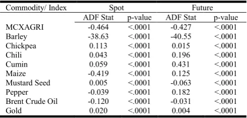
[image:5.595.40.285.290.407.2]test (ADF), which is represented in the Table 1. For all the commodities, the ADF test showed significantly low p-values. As a result, the null hypothesis of presence of unit root was rejected at the 1 % level of significance. The absence of unit root in these series had ensured the stationarity of these series.
Table 1. ADF test results for the returns of the commodities
Commodity/ Index Spot Future
ADF Stat p-value ADF Stat p-value
MCXAGRI -0.464 <.0001 -0.427 <.0001
Barley -38.63 <.0001 -40.55 <.0001
Chickpea 0.113 <.0001 0.015 <.0001
Chili 0.043 <.0001 0.196 <.0001
Cumin 0.059 <.0001 0.431 <.0001
Maize -0.419 <.0001 0.125 <.0001
Mustard Seed 0.005 <.0001 -0.063 <.0001
Pepper -0.039 <.0001 0.182 <.0001
Brent Crude Oil -0.120 <.0001 -0.031 <.0001
Gold 0.020 <.0001 0.004 <.0001
To encounter the fluctuation of the returns of the commodities and the index MCXAGRI volatility was calculated. To calculate volatility, a return series was subdivided into a number of quarterly series. So, for each commodity, a return series (spot or futures) was obtained for each quarter. Volatility was calculated using the data series of each quarter. Entropy as a measure of volatility was used in this paper. Usually, standard deviation, as a measure of volatility, is widespread in the literature. But entropy involves higher moments of the distributions of the data and gives more appropriate estimation of the uncertainty of the data. The entropy was estimated using the Equation 3. For each and every commodities and commodity index volatility was calculated for every quarter by using entropy. To get a better understanding of the behaviour of volatility, for each commodity, spot and futures prices volatility was plotted in the figures Figure 1 to Figure 10. Figure 1 represents the plot of the volatility of MCXAGRI spot and futures prices. From the figure it was observed that the volatility of futures prices was higher than spot prices in most of the quarter. So the futures prices had greater fluctuations than the spot prices. A decreasing trend of volatility was observed for both spot and futures volatility. The volatility of the spot index was highest in the third quarter 2006 and lowest in the second quarter of 2009. For futures series, the highest volatility was observed in the third quarter of 2006 and lowest in the fourth quarter of 2009. For Barley, no trend was observed in the spot and futures price volatility. For the spot prices, highest volatility was observed in the second quarter of 2007 and lowest in the first quarter of 2012. Barley futures prices showed highest and lowest volatility in the third quarter
of 2012 and second quarter of 2008 respectively. No increasing or decreasing trend was observed in the volatility of the commodity Chickpea for both spot and Futures prices. Highest and lowest volatility of the spot prices was observed in the third quarter of 2010 and third quarter of 2006 respectively. For the Chickpea futures prices, highest volatility was observed in the fourth quarter of 2009 and lowest volatility in the first quarter of 2006. For the Chili spot prices, highest volatility was observed in the third quarter of 2012 and lowest in the first quarter of 2007. Chili futures prices showed highest and lowest volatility in the first quarter of 2006 and first quarter of 2011 respectively. Cumin futures showed an increasing trend of volatility. For spot prices the trend was not significant. For the Cumin spot prices, highest volatility was observed in the second quarter of 2007 and lowest volatility in the second quarter of 2008. For the futures prices, highest volatility was observed in the second quarter of 2011 and lowest volatility in the third quarter of 2005. The trend of volatility was decreasing for Maize spot prices. The Maize futures prices showed slightly increasing trend of volatility. The spot prices showed highest and lowest volatility respectively in the third quarter of 2005 and in the fourth quarter of 2011. Maize futures prices had reached highest peak of volatility in both the periods first quarter of 2007 and first quarter of 2008. The volatility was lowest in the fourth quarter of 2011. For Mustard Seed, no trend was observed in the spot and futures prices volatility. For the spot prices, highest volatility was observed in the third quarter of 2010 and lowest in the first quarter of 2011.
The futures prices showed highest volatility in the second quarter of 2006 and fourth quarter of 2009 while the lowest volatility was observed in the first quarter of 2011. For the Pepper spot prices, highest volatility was observed in the second quarter of 2010 and lowest in the fourth quarter of 2010. Pepper futures prices showed highest and lowest volatility in the second quarter of 2008 and second quarter of 2004 respectively. The volatility of the futures prices of Brent Crude Oil was having higher magnitude than the spot prices. Highest spot price volatility was observed in the third quarter of 2008 whereas the lowest volatility was found in the first quarter of 2011 and third quarter of 2012. Highest futures price volatility was observed in the fourth quarter of 2007 and lowest value observed in the first quarter of 2010. The volatility was found to be highest in the third quarter of 2008 for the Gold spot prices. It attained the lowest value in the third quarter of 2007. For the gold futures prices, in the fourth quarter of 2012 the volatility was highest and in the fourth quarter of 2009 it was found to be lowest.
For some of the commodities, trend of volatility was identified by visual inspection of the figures. So, to confirm the existence of trend Mann-Kendall’s Trend Test was used in this paper. The null and the alternative hypotheses of this test were specified as follows:
H0 : No monotonic trend is present in the volatility of the spot
(or futures) prices of a commodity.
Against the alternative,
H1 : Monotonic trend is present in the volatility of the spot (or
futures) prices of a commodity.
Fig. 1. Volatility of the spot and futures prices of MCXAGRI for each quarter
[image:6.595.135.458.524.741.2]Fig. 2. Volatility of the spot and futures prices of Barley for each quarter
Fig. 3.Volatility of the spot and futures prices of Chickpea for each quarter
Fig. 4. Volatility of the spot and futures prices of Chili for each quarter
Fig. 5. Volatility of the spot and futures prices of Cumin for each quarter
[image:7.595.133.456.540.753.2]Fig. 7. Volatility of the spot and futures prices of Mustard Seed for each quarter
Fig. 8. Volatility of the spot and futures prices of Pepper for each quarter
Fig. 9. Volatility of the spot and futures prices of Brent Crude Oil for each quarter
[image:8.595.136.462.544.767.2]Table 2 represents the results of the Mann-Kendall’s trend test for the commodities under this study. For MCXAGRI, both spot and futures prices volatility showed decreasing trend. The p-value was less than 0.05 for the Mann-Kendall’s trend test in these cases. In case of Barley, spot price volatility did not show any trend but futures price volatility had showed an increasing trend. The existence of trend was confirmed by the test as the p-value is less than 0.05. For the commodities chickpea and Chili no trend was identified in the spot and futures volatility series. Again, for Cumin futures prices a trend of volatility was observed by the test. In this case the trend was increasing. However, Cumin spot prices did not show any trend. The volatility of Maize spot prices was having a decreasing trend. The p-value of this test was 0.001. For futures prices no such trend was observed. Volatility of the spot and the futures prices for the commodities Mustard Seed, Pepper, Brent Crude Oil and Gold was free from trend.
Table 2. Results of the Mann-Kendall’s trend test for volatility
Commodity/ Index Spot Future
Kendall's tau p-value Kendall's tau p-value
MCXAGRI -0.464 0.007 -0.427 0.010
Barley -0.243 0.112 0.383 0.010
Chickpea 0.113 0.402 0.015 0.925
Chili 0.043 0.773 0.196 0.151
Cumin 0.059 0.666 0.431 0.001
Maize -0.419 0.001 0.125 0.344
Mustard Seed 0.005 0.976 -0.063 0.609
Pepper -0.039 0.755 0.182 0.129
Brent Crude Oil -0.120 0.392 -0.031 0.837
Gold 0.020 0.916 0.004 1.000
So, for the index MCXAGRI, spot and futures prices volatility behave similarly. In both the cases, trend of volatility was observed. The commodities Chickpea, Chili, Mustard Seed, Pepper, Brent Crude Oil and Gold, also had behaved similar in term of the behaviour of volatility.
For all of these commodities, volatility of the spot and futures prices was free from trend. However, Barley, Cumin and Maize represented a different scenario. For all the commodities, between spot and futures prices, volatility of one of the series was having trend. Then, effort was given to find out if there was any difference between the magnitude of the volatility of spot and futures prices. Two sample t-test was applied to identify if spot and futures prices volatility is significantly different from each other. However, to apply the t-test the sample observations need to follow a normal distribution. So, the normality of the spot and futures prices volatility series was needed to be checked. Shaprio-Wilk Normality Test was used in this purpose. For a commodity, spot price volatility for all the quarters together was considered as the first sample and all the futures prices volatility together was considered as second sample.
For each sample normality was checked by Shaprio-Wilk Normality Test. The hypotheses under this test were given by:
H0 : The distribution of the spot (or futures) prices volatility for
a commodity is normal.
Against the alternative,
H1 : The distribution of the spot (or futures) prices volatility for
a commodity is non-normal.
The results of this test were represented in Table 3. It was observed that for the index MCXAGRI, both the samples did not follow a normal distribution. In both the cases, p-values were less than 0.05. So, the null hypothesis of normality was rejected at the 5 % level. For Mustard Seed also both the samples of volatility did not follow normal distribution. For Maize futures prices volatility did not follow normal distribution. However, volatility of the Maize spot prices was found to follow normal distribution. For all other commodities both the samples had followed normal distribution.
Fig. 10. Volatility of the spot and futures prices of Gold for each quarter
[image:9.595.36.290.545.696.2]Since, the volatility samples had followed both normal and non-normal distributions, both parametric and non-parametric tests were used to check if the volatility of spot and futures prices was significantly different from each other. Among the two sample parametric tests, the Welch’s t-test was used in this purpose. Also, Kolmogorov-Smirnov non-parametric test was applied for a better inference of the non-normal samples. The hypotheses considered in the Welch’s t-test were given by:
H0 : µSpot = µFutures
Against the alternative,
H1 : µSpot ≠ µFutures
Where,
µSpot = mean volatility of the spot prices of a commodity
µFutures = mean volatility of the futures prices of a commodity
For Kolmogorov-Smirnov two sample test the hypothesis under consideration were:
H0 : FSpot = FFutures
Against the alternative,
H1 : FSpot ≠ FFutures
Where,
FSpot = probability distribution of volatility of the spot prices of
a commodity
FFutures = probability distribution of volatility of the futures
prices of a commodity
Table 4 contains the results of two sample tests. For the commodities Chickpea, Chili and Gold the spot and futures price volatility were significantly different at 5% level as the p-values in these cases were lesser than 0.05. Both the parametric and non-parametric tests had provided the same results. For all other commodities no significant difference was found between the spot and futures price volatility. So, for most of the commodities spot and futures market volatility was similar. That means, spot and futures market reacts in a similar way to new information. This is an indication of the fact that spot and futures markets are associated. For, Chickpea, Gold and Brent Crude Oil, the volatility of spot and futures market was significantly different from each other. That mean one of the markets is more volatile than other market.
For the commodities Chickpea, Chili and Gold spot and futures prices volatility was significantly different. So, for these commodities, it was checked that which market was having greater volatility in between spot and futures markets. Since for these three commodities the volatility series had followed normal distribution, in this purpose Welch’s t-Test was used again. However, this time one-sided alternative hypothesis was used. The hypotheses considered in this test were given by:
H0 : µSpot = µFutures
Against the alternative,
H1 : µSpot > µFutures or H2 : µSpot < µFutures
Where,
µSpot = mean volatility of the spot prices of a commodity
µFuture = mean volatility of the futures prices of a commodity
Table 5 depicts the results of Welch’s t-Test with one-sided alternative. In case of Chickpea spot prices volatility was higher than the futures price volatility. The observation was same for gold also. However, for Chili spot market was having lower volatility compared to the futures market.
Then, to judge the behaviour of volatility, the variation of the spot and futures price volatility for different commodities was needed to be analysed. In this purpose two sample variance test was useful. F-test was applied to check whether the variability of the spot and futures price volatility was same. Since, some of the volatility samples had followed non-normal distribution and F-test requires the data set to be normally distributed, so with the F-test a non-parametric test was also used in this regard. Levene’s Test was used to compare the variances of the two samples of volatility. The hypotheses considered in these tests were given by:
H0 : σ2Spot = σ2Futures
Against the alternative,
H1 : σ2Spot ≠ σ2Futures
Where,
σ2Spot = variance of the volatility of spot prices of a commodity
σ2Futures = variance of the volatility of futures prices of a
commodity
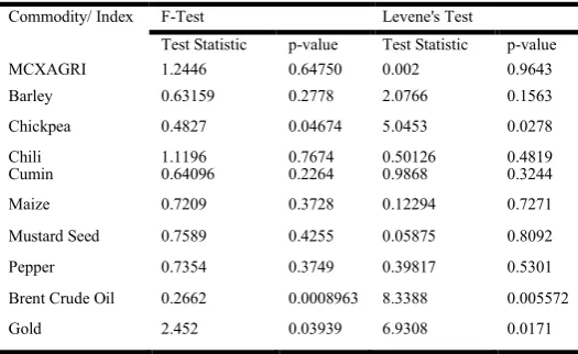
The results of the F-Test and the Levene’s Test were depicted in Table 6. It was observed that for Chickpea, Brent Crude Oil and Gold, the p-values were smaller than 0.05. Therefore, for these commodities, the variation of spot and futures price volatility was significantly different from each other. For the commodities other than these three, the variation of volatility was similar in the spot and futures market.
Then, it was to be checked that between spot and futures which market was having a higher variation of volatility. For the commodities Chickpea, Brent Crude Oil and Gold, the variations of spot and futures price volatility were significantly different. So, for these commodities, it was checked that which market was having a greater variation of volatility in between spot and futures markets. For these commodities spot and futures prices volatility samples had followed normal distribution. So, in this purpose F-test was used with the one-sided alternative hypothesis. The hypotheses considered in this test was given by:
H0 : σ2Spot = σ2Futures
Against the alternative,
H1 : σ2Spot > σ2Futures or H2 : σ2Spot < σ2Futures
Where,
σ2Spot = variance of the volatility of spot prices of a commodity
σ2Futures = variance of the volatility of futures prices of a
[image:11.595.33.293.105.259.2]commodity
Table 3. Results of the Shapiro-Wilk Test for Normality
Commodity/ Index Spot Future
Test Statistic p-value Test Statistic p-value
MCXAGRI 0.885916 0.027 0.882423 0.024
Barley 0.929612 0.096 0.977821 0.853
Chickpea 0.984283 0.902 0.915113 0.12
Chili 0.946519 0.162 0.967208 0.487
Cumin 0.966014 0.417 0.951811 0.162
Maize 0.982157 0.87 0.863567 0.001
Mustard Seed 0.898823 0.004 0.877067 0.001
Pepper 0.962169 0.265 0.973411 0.543
Brent Crude Oil 0.939738 0.099 0.93448 0.089
[image:11.595.308.560.119.179.2]Gold 0.982392 0.936 0.921221 0.071
Table 4. Results of the two sample tests for the equality of means between spot and futures prices volatility
Commodity/ Index Kolmogorov-Smirnov Test Welch t-Test
Test Statistic p-value Test Statistic p-value
MCXAGRI 0.42105 0.06809 -1.3083 0.19920
Barley 0.41667 0.13101 -1.7205 0.09240
Chickpea 0.93636 0.00000 -10.429 0.00000
Chili 0.83005 0.00976 -3.006 0.00400
Cumin 0.15423 0.84800 0.27796 0.78200
Maize 0.30242 0.11220 0.30075 0.76460
Mustard Seed 0.31429 0.06304 -1.0993 0.13958
Pepper 0.28571 0.11480 1.3336 0.18690
Brent Crude Oil 0.22733 0.46520 -0.94187 0.35220
Gold 0.40761 0.04038 2.4714 0.01789
Table 5. Results of the two sample Test for the equality of means between spot and futures prices volatility
Commodity/ Index Welch t-Test
Alternative Hypothesis Test Statistic p-value
Chickpea µSpot > µFutures -10.429 0.00000
Chili µSpot < µFutures -3.006 0.00200
Gold µSpot > µFutures 2.4714 0.00895
Table 6. Two sample tests for the equality of variance between spot and futures prices volatility
Commodity/ Index F-Test Levene's Test
Test Statistic p-value Test Statistic p-value
MCXAGRI 1.2446 0.64750 0.002 0.9643
Barley 0.63159 0.2778 2.0766 0.1563
Chickpea 0.4827 0.04674 5.0453 0.0278
Chili 1.1196 0.7674 0.50126 0.4819
Cumin 0.64096 0.2264 0.9868 0.3244
Maize 0.7209 0.3728 0.12294 0.7271
Mustard Seed 0.7589 0.4255 0.05875 0.8092
Pepper 0.7354 0.3749 0.39817 0.5301
Brent Crude Oil 0.2662 0.0008963 8.3388 0.005572
Gold 2.452 0.03939 6.9308 0.0171
The results of F-test with a one-sided alternative were depicted in Table 7. Chickpea had shown that the variation of spot price
[image:11.595.37.287.298.407.2]volatility was lesser than the variation of futures price volatility.
Table 7. Two sample test for the equality of variance between spot and futures prices volatility
Commodity/ Index F-Test
Alternative Hypothesis Test Statistic p-value
Chickpea σ2
Spot < σ2Futures 0.4827 0.02337
Brent Crude Oil σ2
Spot < σ2Futures 0.26626 0.0004482
Gold σ2Spot > σ2Futures 2.452 0.01969
The observation was similar for Brent Crude Oil as well. However, for Gold the variation of the volatility of the spot market was having higher value compared to the futures market.
DISCUSSION
The results of this study have indicated few facts regarding the volatility of the Indian commodity market. For most of the commodities no trend is observed in the spot and the futures price volatility. However, for some of the commodities trend of volatility is observed. Evidence of both increasing and decreasing trend is observed in these cases. Also the nature of trend is not similar for spot and futures price volatility of these commodities except for the index MCXAGRI. So, no particular pattern in the trend of volatility is observed in the Indian commodity market. So, the common belief of the investors, that the introduction of derivative trading in the commodity market has increased the volatility of the market cannot be justified by the results of this study.
Again, for most of the commodities spot and futures price volatility is having similar values. Both parametric and non-parametric tests confirm the result. However, for some of the commodities, namely Chickpea, Chilli and Gold, spot and futures price volatility is significantly different. For Chickpea spot market is having higher volatility than futures market and for Gold the scenario is opposite. Additionally, the variation of volatility is similar in spot and futures prices for most of the commodities. Only contradictory results have been found for Chickpea, Brent Crude Oil and Gold. For Chickpea and Brent Crude Oil, the spot market is having lesser variation while for Gold the futures market is having a lesser variation of volatility. So, the magnitude and the variability of volatility is similar in spot and futures prices for most of the commodities in the Indian commodity market. However, exceptions are there for some the commodities. Both spot and futures markets for commodities are expected to behave similar and help each other in evolution. Dissemination of information between the markets should help in the effective price discovery in both the markets. To be efficient commodity market co-movements of the spot and futures markets is necessary. In the Indian market also similar facts have been observed with some exceptions.
Conclusion
In the Indian commodity market, insufficient evidences have been found in support of the fact that the introduction of derivative trading has increased the volatility of the market.
[image:11.595.32.291.449.498.2] [image:11.595.31.294.539.700.2]Though trend is present in the volatility of the commodities but no specific pattern of trend is found. Furthermore, in respect of trend, volatility of the spot and futures market has a similar pattern with few exceptions. The average volatility of the spot and futures prices is found to be same in most cases. The pattern of change of volatility over time is also similar in both the markets for most of the cases. These facts indicate an association between the spot and futures markets for the commodities in India. The more spot and futures markets for commodities are associated the more efficient they will be.
REFERENCES
Adrian, T. and Rosenberg, J. 2008. Stock Returns and
Volatility: Pricing the Short-Run and Long-Run
Components of Market Risk, The Journal of Finance,
63(6): 2997–3030.
Bagchi, D. 2007. An Analysis of Relative Information Content of Volatility Measures of Stock Index in India. ICFAI Journal of Derivatives Markets, 4(4): 35-43.
Bandivadekar, S. and Ghosh, S. 2003. Derivatives and Volatility on Indian Stock Markets. Reserve Bank of India Occasional Papers, 24(3).
Dionisio, A., Menezes, R. and Mendes, D.A. 2006. An econophysics approach to analyse uncertainty in financial markets: an application to the Portuguese stock market. The European Physical Journal B - Condensed Matter and Complex Systems, 50: 161-164.
Granger, C. and Lin , J. 1994. Using the Mutual Information Coefficient to Identify Lags in Nonlinear Models. Journal of Time Series Analysis, 15(4): 371-384.
Haugen, R. A., Talmor, Eli., and Torous, W. 1991. The Effect of Volatility Changes on the Level of Stock Prices and Subsequent Expected Returns. The Journal of Finance, 46(3): 985–1007.
Maasoumi, E. 1993. A Compendium to Information Theory in
Economics and Econometrics. Econometric Reviews,
12(2): 137-181.
Maasoumi, E., Ebrahimi, N. and Soofi, E. 1999. Ordering univariate distributions by entropy and variance. Journal of Econometrics, 90: 317-336
Pal, P. 2005. Volatility in the Stock Market in India and Foreign Institutional Investors: A Study of the Post-Election Crash. Economic and Political Weekly, 40(8): 765-772.
Pindyck, R. S. 2004. Volatility And Commodity Price
Dynamics. The Journal of Futures Markets, 24(11): 1029–
1047.
Raju, M. T. and Ghosh, A. 2004. Stock Market Volatility – An International Comparison. Working Paper Series No. 8, Securities and Exchange Board of India.
Shannon, C. E. 1948. A Mathematical Theory of Communication, Bell Systems Tech., 27: 379-423, 623-656.
Soofi, E. 1997. Information Theoretic Regression Methods,
Fomby, T. and R. Carter Hill ed: Advances in Econometrics
- Applying Maximum Entropy to Econometric Problems,
12, Jai Press Inc., London.
Urbach, R. 2000. Footprints of Chaos in the Markets - Analysing non-linear time series in financial markets and other real systems, Prentice Hall, London.