The Properties and Fast Algorithm of Quaternion Linear Canonical Transform

(1)

http://www.scirp.org/journal/jsip ISSN Online: 2159-4481

ISSN Print: 2159-4465

DOI: 10.4236/jsip.2018.93012 Aug. 21, 2018 202 Journal of Signal and Information Processing

The Properties and Fast Algorithm of

Quaternion Linear Canonical Transform

Ye Zhang

1

, Guanlei Xu

2*

1_{Nanjing Changjiang Electronics Group Co. Ltd., Nanjing, China} 2_{Dalian Navy Academy, Dalian, China}

Abstract

The quaternion linear canonical transform (QLCT) is defined in this paper, with proofs given for its reversibility property, its linear property, its odd-even invariant property and additivity property. Meanwhile, the quater-nion convolution (QCV), quaterquater-nion correlation (QCR) and product theo-rem of LCT are deduced. Their physical interpretation is given as classical convolution, correlation and product theorem. Moreover, the fast algorithm of QLCT (FQLCT) is obtained, whose calculation complexity for different signals is similar to FFT. In addition, the paper presents the relationship be-tween the convolution and correlation in LCT domains, and the convolution and correlation can be calculated via product theorem in Fourier transform domain using FFT.

Keywords

Quaternion Signals (Hyper-Complex Signals), LCT, Convolution, Correlation

1. Introduction

The linear canonical transform (LCT) is a new tool that comes into being in sig-nal processing [1]-[32]. The LCT is the generalization of the FRFT and so on [2] [3] [12]. Up till now there have been a lot of papers involving the FRFT and the LCT, such as papers [1]-[10]. However, none of them has involved the LCT of quaternion signals (or Hyper-complex signals) even if there has been similar work on FRFT [5]. Quaternion signals can be taken as the generalization of sca-lar, complex signals and vector, and after the introduction of quaternion signals by Hamilton in 1843 [11] it has become one basic tool for multi-channel and multi-dimensional space. For example, grey image [30] can be taken as scalar, and the analytic signal after Hilbert transformation [12] [13] [14] [15] [16] [29]

How to cite this paper: Zhang, Y. and Xu, G.L. (2018) The Properties and Fast Algo-rithm of Quaternion Linear Canonical Transform. Journal of Signal and Informa-tion Processing, 9, 202-216.

https://doi.org/10.4236/jsip.2018.93012

Received: June 28, 2018 Accepted: August 18, 2018 Published: August 21, 2018

http://creativecommons.org/licenses/by/4.0/

(2)

DOI: 10.4236/jsip.2018.93012 203 Journal of Signal and Information Processing

is complex signal. The color image can be taken as one vector [17] [18], a qua-ternion number whose real part is zero. In [19], the transform, convolution and correlation have been addressed in fractional Fourier transform (FRFT) domain. In this paper we first propose the definition of the QLCT, QCV and QCR in the LCT domain for quaternion signals, which are the generalization of those in [5]. Meanwhile, some properties and the fast algorithm of QLCT are discussed. We also discover the relationship of QCV and QCR in the LCT domain for quater-nion signals. We found that QCV and QCR can be implemented via product theorem in the QLCT domain. Thus we not only yield the generalized frame for scalar, complex signal, vector and quaternion signal [17] [20] in the QLCT do-main, but also give one new idea and one theoretical base for future engineering use.

In the rest of this paper, we will introduce the definition of QLCT in Section II. We will show the properties in Section III. In Section IV, FRQCV and FRQCR will be addressed. Section V is the fast algorithm. The last section con-cludes our paper.

2. Definitions of QLCT

For convenience of discussion, we first give some notations used in the following of this paper. f x y

( )

, denotes 2D signal in time domain; F is classical Fourier

transform operator; L a b c d( , , , )

F (_FL in short) is 1D LCT operator, and L

( )

F u

is the 1D LCT of f x y

( )

, ; _FL L1, 2 is the 2D LCT operator of _{f x y}

( )

_, ; _FQ is classical quaternion Fourier transform operator, and Q

( )

,

F u v is quaternion Fourier transform of f x y

( )

, ; I is equivalence operator; P is odd-even operator;

“*” is classical convolution operator; “−_{” is conjugation operator. “}_N_{” is integer} set; “R” is real set. Define the product operator of two LCTs’ transform parame-ter systems:

(

) (

)

(

)

1 2 1 1, , ,1 1 1 2 2, 2, 2, 2 , , ,

L L =L a b c d ⋅L a b c d =L a b c d

where 1 1 2 2

1 1 2 2

a b a b

a b

c d c d

c d

   

 

=    

 

     . Quaternion signals are also called Hyper- complex signals, which are the generalization of complex signals. Complex sig-nals have two components: the real part and the imaginary part. However, one quaternion signal has four parts, one real component and three imaginary parts:

r i j k

q=q +iq + jq +kq (1) where q q q qr, ,i j, k∈R, i j k, , are three imaginary units, which satisfy the fol-lowing relations: 2 2 2

1

i = j =k = − , ij= − =ji k, jk= − =kj i , ki= − =ik j .

a r i

q =q +iq, qb= +qi iqk. If qr =0, then q=iqi+ jqj+kqk is called vector, and qr is called scalar. qa and qb are complex signals. Since the sequences of i, j and k will affect the result, the definition of QLCT would take them into account.

Definition 1: For any quaternion signal

( )

, r

( )

, i

( )

, j

( )

, k

( )

,

(3)

( )

,

j

f x y , fk

( )

x y, are real ones), the QLCT of f x y

( )

, is

( )

1, 2

, ,

L L i j

F u v

( )

{

(

)

}

{

(

)

}

( )

( ) (

)

( )

1 2 1 2 1 2

1 2

, , ,

, ,

, , , ,

, , , d d

L L L L L L

i j i j i j

L i L j

F u v F f x y F f x y u v

K x u f x y K y v x y

+∞ +∞

−∞ −∞

= =

=

_{∫ ∫}

(2-1)

where, 1

( )

(

)

2 1 1 ,

1 1 1

1

, exp

2π 2

L i

a d u ux

K x u i i

b i b b

 + 

= _ − _

 ,

( )

(

)

2

2 2 2 ,

2 2 2

1

, exp

2π 2

L j

a d v vy

K y v j j

b j b b

 + 

= _ − _

 . Meanwhile, in the following of

this paper we assume a d1 1−b c1 1=1, a d2 2−b c2 2=1 and b b1, 2≠0.

The reversibility transform is defined as

( )

{

(

)

}

{

(

)

}

( )

( ) (

)

( )

1 2 1 2 1 2

1 2

, , ,

, ,

, , , ,

, , , d d

L L L L L L

i j i j i j

L i L j

F u v F f x y F f x y u v

K x u f x y K y v x y

− − − − − −

+∞ +∞

− −

−∞ −∞

= =

=

_{∫ ∫}

(2-2)

where, 1

( )

(

)

2 1 1 ,

1 1 1

1

, exp

2π 2

L i

a d u ux

K x u i i

b i b b

−

 + 

= _− + _

− _ _,

( )

(

)

2

2 2 2 ,

2 2 2

1

, exp

2π 2

L j

a d v vy

K y v j j

b j b b

−

 + 

= _− + _

− _ _.

If

(

a b c d1, , ,1 1 1

) (

= a b c d2, , ,2 2 2

) (

= 0, 1,1, 0−

)

, definition 1 is quaternion Fourier

transform; if

(

a b c d1, , ,1 1 1

) (

= 0, 1,1, 0 ,−

) (

a b c d2, , ,2 2 2

) (

= 1, 0, 0,1

)

, definition 1 is

classical 1D Fourier transform of f x y

( )

, for variable x; if

(

a b c d1, , ,1 1 1

) (

= 1, 0, 0,1

)

,

(

a b c d2, 2, 2, 2

) (

= 0, 1,1, 0−

)

, definition 1 is classical 1D

Fourier transform of f x y

( )

, for variable y; if

(

a b c d1, , ,1 1 1

) (

= a b c d2, 2, 2, 2

) (

= 1, 0, 0,1

)

, definition 1 is equivalence transform of

( )

,

f x y . As shown above, definition 1 is the generalization of the fractional qu-aternion Fourier transform and the ququ-aternion Fourier transform [18] [19] [20] [21]. The reversibility (or reconstruction) is one important property for one transform, especially for the processing in another domain. The following gives the proof of the reversibility property.

Theorem 1: One quaternion f x y

( )

, can be reconstructed from 1, 2

( )

, ,

L L i j

F u v

via QLCT.

Proof: The proof is trivial and omitted here.

3. The Properties of QLCT

In the following section we list the properties and present the proof.

Property 1: For any one quaternion signal fn

( )(

x y n, ∈ℵ

)

, the following

re-lationship is true: 1, 2

{

(

)

}

1,2

{

(

)

}

, , , ,

L L L L

i j n n n i j n

F

∑

a f x y =

∑

a ⋅F f x y

(

an∈ℜ

)

. Proof: Since QLCT is one linear transform, property 1 can be easily obtained from definition 1.

Property 2: 3,4 1,2 1, 2 3,4 1 3, 2 4

, , , , ,

L L L L L L L L L L L L

i j i j i j i j i j

F F =F F =F . Proof: For any one

(4)

( )

{

}

( )

( ) ( )

( )

(

)

( )

( ) ( )

( )

(

)

( )

3 4 1 2

3 1 2 4

3 1 , , , , , , , , , , , , , , ,

, , , , d d , d d

, , , , , d d d d

, , d ,

L L L L i j i j

L i L i L j L j

L i L i L

F F f x y

K u s K x u f x y K y v x y K v w u v

K u s K x u f x y K y v K v w u v x y

K u s K x u u f x y K

+∞ +∞ +∞ +∞ −∞ −∞ −∞ −∞ +∞ +∞ +∞ +∞ −∞ −∞ −∞ −∞ +∞ −∞   =       =       = _ _  

∫ ∫

∫ ∫ ∫ ∫

∫

2,j

( )

y v K, L4,j

(

v w,

)

dv d dx y

+∞ +∞ +∞ −∞ −∞ −∞             

∫ ∫

∫

(3) For 1D signal the right formula is true [2]:

(

) (

)

(

)

2 , 1 , d 2 1 ,

L L L L

K u u K u u u K u u

+∞

−∞

′ ′ ′′ ′′= ′′

∫

(4)

Substitute (4) into (3):

(

)

{

}

( ) (

)

(

)

{

}

{

(

)

}

3 4 1 2

1 3 2 4

3 1 4 2

, , , ,

,

, , ,

,

, , , d d ,

L L L L i j i j

L L L L

L L i L L j i j

F F f x y

K x s f x y K y w x y F f x y

+∞ +∞

−∞ −∞

=

_{∫ ∫}

=

Therefore,

3,4 1,2 1 3,2 4

, , ,

L L L L L L L L

i j i j i j

F F =F (5)

The result can be obtained similarly:

3 4 1 3 2 4

1,2 , ,

, , ,

L L L L L L

L L

i j i j i j

F F =F (6)

From (5) (6): 3,4 1,2 1,2 3,4 1 3,2 4

, , , , ,

L L L L L L L L L L L L

i j i j i j i j i j

F F =F F =F

Property 3: 3,4 1, 2 1,2 3,4

, , , ,

L L L L L L L L

i j i j i j i j

F F =F F ,

(

) (

)

5,6 3,4 1,2 5,6 3,4 1,2

, , , , , ,

L L L L L L L L L L L L

i j i j i j i j i j i j

F F F = F F F .

Proof: This property can be obtained from property 2. Property 4: If 1,2

{

(

)

}

1, 2

( )

, , , ,

L L L L

i j i j

F f x y =F u v , then

(

)

{

}

(

)

1,2 1,2

, , , ,

L L L L

i j i j

F f − −x y =F − −u v , 1, 2

{

(

)

}

1,2

(

)

, , , ,

L L L L

i j i j

F f −x y =F −u v ,

(

)

{

}

(

)

1,2 1, 2

, , , ,

L L L L

i j i j

F f x−y =F u −v .

Proof: Let A1= 2πb i1 , A2= 2πb j2 ,

1 1 1 2 d C b

= _, 2

2 2 2 d C b

= _{, and insert them} into (2):

(

)

{

}

2 2

(

)

2 2

1,2 1 1 1 1 2 2

, , 1e e e , e e d d 2e

ux vy

i j

L L iu C b ix C jy C b jv C

i j

F f x y A f x y x y A

+∞ +∞ − −

−∞ −∞

− − =

_{∫ ∫}

− − ⋅ (7)

Let s= −x z, = −y, and substitute them in (7):

(

)

{

}

{

( )

}

( )

( ) ( ) ( )

_{( )}

( ) ( )

(

)

1 2 1 2

2 2 2 2

1 1 1 2 2 2

2 2 2 2

1 1 1 2 2 2

1 2 , , , , 1 2 1 2 , , , ,

e e e , e e d d e

,

L L L L

i j i j

u s v z

i j

iu C b is C jz C b jv C

u s v z

i j

i u C b is C jz C b j v C

L L i j

F f x y F f s z

A f s z s z A

F u v

(5)

It can be obtained as well: 1,2

{

(

)

}

1, 2

(

)

, , , ,

L L L L

i j i j

F f −x y =F −u v and

(

)

{

}

(

)

1,2 1, 2

, , , ,

L L L L

i j i j

F f x−y =F u −v .

We can draw the conclusion that transformed signal of the odd is odd, and even is even.

Property 5: If n∈ℵ, then

(

1,2

)

( ) ( )1 , 2

, ,

n n

n _L _L

L L

i j i j

F =F .

Proof: From property 2,

( ) ( )

1 1 2 2

1 2

1 2 1 2 1 2

,

, , ,

, , , , ,

n n

L L L L

p p

L L L L L L

i j i j i j i j i j

n

F F F F F

× × × ×

= =

 

 

 

then

(

1,2

)

( ) ( )1 , 2

, ,

n n

n _L _L

L L

i j i j

F =F .

QLCT doesn’t satisfy Parseval’s principle. Meanwhile, it is hard to find one obvious relationship between QLCT and Wigner-Ville time-frequency plane. Some other properties [2] cannot find physical interpretation in QLCT domains.

4. FRQCV and FRQCR

Convolution and correlation play an important role in signal processing, espe-cially for linear system design and filter design, etc. The convolution in time domain is to the product in Fourier transform domain, that is to say, the classic-al convolution in time domain can be implemented in Fourier transform do-main via FFT, which is beneficial for real-time engineering use. In classical time-frequency analysis correlation is special convolution in that the original signals are implemented via conjugation and so on. This is very important for engineering use [17] [20] [24]. The key to this paper is to discover the relation-ships in fractional quaternion Fourier transform domain between them so that we can find the physical interpretation as that of the classical Fourier transform. Paper [26] yielded fractional convolution and product theorem for 1D signals first, however, it didn’t give the similar physical interpretation as that of the clas-sical theorem. Later papers [27] [28] [29] obtained similar result as the classical theorems. However, they are only for 1D signals. In this section the QCV and QCR of the LCT would be discussed, and can be implemented via FFT.

4.1. Fractional Convolution and Product Theorem

In the following, four theorems are yielded, and theorem 2 and 3 are suitable for scalar and complex signals, and theorem 4 and 5 are suitable for scalar, complex signals, vector and quaternion signals.

Theorem 2: For any real scalar or complex signal f x y

( )

, and convolution

kernel h x y

( )

, ,

( )

( ) ( ) (

)( )

(

2 2

) (

2 2

)

_{( )}

(

2 2

)

1 2 1 2 1 2

1,2

, , , ,

ei x C y C ei x C y C , , ei x C y C g x y f x y h x y f h x y

A − + + f x y h x y +

= ∗ = ∗

  _∗ 

   

   

(6)

where B1=1b1, B2=1b2, 1,2

1 2

1 2π

A

i b b

= _, 1

1 1 2 a C b

= _, 2

2 2 2 a C b

= _{, then:}

( )

{

}

(

2 2

)

{

( )

}

{

( )

}

1 2

1,2 _, _e i u C v C 1,2 _, 1, 2 _,

L L L L L L

F g x y = − + F f x y ⋅F h x y (8)

Proof:

(

)

{

}

(

) (

)

(

)

(

)

(

)

( )

(

)

₍

₎

₍

₎

(

)

1 2 1 2

2 2 2 2 2 2

1 2 1 2 1 2 ₁ ₂

2 2 2 2

1 2 1 2

,

1,2 1,2

, , , , , d d

e e e e

e , , e d d

L L

i u C v C i x C y C i x C y C i xuB yvB

i x C y C i x C y C

F g x y K x y u v g x y x y

A A

f x y h x y x y

+∞ +∞ −∞ −∞ +∞ +∞ + + − + ₋ ₊ −∞ −∞ + + = =     ⋅_ _{ }∗ _    

∫ ∫

(9)

Substitute (9) with s= −x

τ

,z= −y

η

:

( )

{

}

(

)

(

)

( )

(

)

( )

(

)

_{( )}

( )

_{

_{( )}

_}

(

)

_{

_{( )}

_}

2 2 2 2

1 2 1 2 ₁ ₂

1 2

2 2

1 2 ₁ ₂

2 2

1 2 ₁ ₂ ₁ ₂

2 2

1 2 ₁ ₂ ₁

, 2

1,2

, 1,2

,

, e e , e

, e e d d d d

e , e d d ,

e ,

i u C v C i C C i uB vB

L L

i s C z C _{i suB} _zvB

i C C _{i uB} _vB _{L L}

i u C v C L L L

F g x y A f

h s z s z

A f F h x y

F f x y F

τ η _τ _η

τ η

τ η τ η

+∞ +∞ + + ₋ ₊ −∞ −∞ +∞ +∞ + − + −∞ −∞ +∞ +∞ + − + −∞ −∞ − + =   ⋅     = ⋅ = ⋅

∫ ∫

( )

{

}

2 , , L

h x y

From theorem 2 it can be concluded that the convolution of scalar or complex signal is to the product, frequency-modulated by a chirp, of them in linear ca-nonical transform.

Theorem 3: For any real scalar or complex signal f x y

( )

, and convolution

kernel h x y

( )

, ,

( )

(

)

( )

(

2 2

)

(

2 2

)

_{( )}

(

2 2

)

1 2 1 2 1 2

, ,

ei x C y C 2π e i x C y C , , ei x C y C

g x y f h x y

f x y h x y

+ − + − + = ∗   _⋅  _∗              

where B1=1b1, B2=1b2, 1,2

1 2

1 2π

A

i b b

= _,

( )( )

1, 1 1,2 1 2 1 2π A

i b b

− − ₌ − − , 1 1 1 2 a C b

= _, 2

2 2 2 a C b

= _{, then}

(

)

_{( ) ( )}

( )

(

)

2 2 1 2 1 2 , ,

1 2 1 2

, 1, 1 1,2

e , ,

, ,

L L L L

i u C v C L L

F f x y g x y

A f u v h u v

+ − −       = ∗ (10) Proof:

( )

(

)

(

)

₍

₎

( )

{

}

( ) 1 2 , ,

1 2 1 2

2 2

1 2

2 2

1 2 ₁ ₂

1 2 1 2

, 1, 1 1,2 1, 1

1,2 1, 1

1,2 , ,

, ,

e

e , , e d d

2π

L L L L

L L

i x C y C

i C u C v _{i xuB} _yvB

L L L L

F A f u v h u v

A

A f u v h u v u v

− − − − − + − − +∞ +∞ − + − − + −∞ −∞ ∗ =

_{∫ ∫}

∗

(7)

( )

{

}

(

)

(

)

_{( )}

(

)

( ) ( )

_{( )}

(

)

( )

_{( )}

1 2

1 2 1 2

2 2

1 2

2 2

1 2 ₁ ₂

1 2 2 2 1 2 1 2 1 2 1 2 1 2

, 1, 1

1,2 , ,

2 1, 1 1,2 , 2 , 1, 1 1,2 , , , e

, e e d d

4π

e , e d d

, e , e

2π

L L

L L L L

i x C y C

i C s C z _{i xsB} _yzB L L

i C C

i x B y B L L

i i x B y B

L L

F A f u v h u v

A

h s z s z

f A

h x y f

τ η

τ η τ η

τ η − − − − − + − − _{+∞ +∞ +∞ +∞} − + ₊ −∞ −∞ −∞ −∞ − + + − − − + ∗   = _ _   ⋅ =

∫ ∫ ∫ ∫

(

)

( ) ( )

(

)

2 2 1 2 2 2 1 2 d d

, , e

C C

i C x C y f x y h x y

τ η τ η +∞ +∞ ₊ −∞ −∞ − + =

∫ ∫

Therefore, ₁ ₂

(

21 2 2

)

( ) ( )

(

( )

)

, ,

1 2 1 2

, 1, 1

1,2

e , , L L , L L ,

i u C v C L L

F  + f x y g x y  = A− − f u v ∗h u v

  .

Theorem 4: For one given quaternion function

( )

, _a

( )

, _b

( )

,

f x y = f x y + f x y j and convolution kernel function

( )

, _a

( )

, _b

( )

,

h x y =h x y +h x y j

where f_a

( )

x y, = f_r

( )

x y, +if x y_i

( )

, , f_b

( )

x y, = f_j

( )

x y, +if_k

( )

x y, ,

( )

,

( )

,

( )

,

a r i

h x y =h x y +ih x y , h x y_b

( )

, =h x y_j

( )

, +ih_k

( )

x y, .

Set 1,2

1 2

1 2π

A

i b b

= _,

( )( )

1, 1 1,2 1 2 1 2π A

i b b

− − ₌

− − , and define

( ) (

)( )

(

2 2

) (

2 2

)

_{( )}

(

2 2

)

1 2 1 2 1 2

1,2

, ,

ei x C y C ei x C y C , , ei x C y C g x y f h x y

A − + + f x y h x y +

= ∗

  _∗ 

   

   



where, 1

1 1 2 a C b

= _, 2

2 2 2 a C b

= _, B₁=1b₁, B2=1b2, α =arcsinb1, β =arcsinb2,

then

( )

{

}

(

)

{

( )

}

(

)

_{

_{( )}

₍

₎

( )

(

)

}

2 2 1 2

1 2 1 2 1 2

1 2 1 2

2 2

1 2 ₁ ₂ ₁ ₂

1 2 1 2

, , ,

, ,

, e , ,

, ,

e , ,

, ,

i u C v C

L L L L L L

a a

L L L L

b b

i u C v C _{L L} _L _L

a b

L L L L

b a

F g x y F f x y F h x y

F f x y F h x y

F f x y F h x y

F f x y F h x y j

α β − + + − − ₋ ₋ − − = _ _⋅ _ _   − _ _⋅ _ _ + _ _⋅ _ − − _   + _ _⋅ _ − − _ ⋅ (11) Proof:

(

)

_{( )}

(

)

(

)

₍

_{( )}

₎

₍

_{( )}

₎

(

)

(

)

_{( )}

(

)

(

)

_{( )}

(

)

2 2 2 2

1 2 1 2

2 2 2 2

1 2 1 2

2 2 2 2

1 2 1 2

2 2 2 2

1 2 1 2

e , , e

e , , , , e

e , , e

e

i x C y C i x C y C

a b a b

i x C y C i x C y C

a a

i x C y C i x C y C

a b

f x y h x y

f x y f x y j h x y h x y j

f x y h x y

f x y h x y j

+ + + + + + + − +   _∗              =_ + _{ }∗ + _         =_ _{ }∗ _         +_ _{ }∗ _⋅     +

(

)

( )

(

)

(

)

_{( )}

(

)

2 2 2 2

1 2 1 2

2 2 2 2

1 2 1 2

, , e

e , , e

i x C y C i x C y C

b a

i x C y C i x C y C

b b

f x y h x y j

f x y h x y

(8)

From theorem 2 it can be obtained

(

) (

)

₍

₎

₍

₎

(

)

(

)

₍

_{

₍

₎

_}

_{

₍

₎

_}

₎

2 2 2 2 2 2

1 2 1 2 1 2

1 2

2 2

1 2 ₁ ₂ ₁ ₂

, 1,2

, ,

e e , , e

e , ,

i x C y C i x C y C i x C y C

L L

a a

i u C v C _{L L} _{L L}

a a

F A f x y h x y

F f x y F h x y

− + + + − +    _∗   _  _{ } _   = ⋅

(

) (

)

_{( )}

(

)

(

)

₍

_{

_{( )}

_}

_{

_{( )}

_}

₎

2 2 2 2 2 2

1 2 1 2 1 2

1 2

2 2

1 2 ₁ ₂ ₁ ₂

, ,

e e , , e

e , ,

L L

b b

i u C v C _{L L} _{L L}

b b

F A f x y h x y

F f x y F h x y

α β − + + − + − +    _∗   _  _{ } _   = ⋅

From the linear property of fractional Fourier transfor

( )

{

}

(

)

_{

_{( )}

( )

}

(

)

_{

_{( )}

₍

₎

( )

(

)

}

1 2 2 2

1 2 ₁ ₂ ₁ ₂

1 2 1 2

2 2

1 2 ₁ ₂ ₁ ₂

1 2 1 2

, , , , , , , , , ,

e , ,

, ,

e , ,

, ,

L L

i u C v C _{L L} _{L L}

a a

L L L L

b b

i u C v C _{L L} _L _L

b b

L L L L

b a

F g x y

F f x y F h x y

F f x y F h x y

F f x y F h x y j

α β − + + − − ₋ ₋ − − = _ _⋅ _ _   − _ _⋅ _ _ + _ _⋅ _ − − _   + _ _⋅ _ − − _ ⋅

From theorem 4 we draw the conclusion that the convolution of two quater-nion signals is to the summation of product of their components, conjugated or odd-even operated, and the product is frequency modulated by chirps. Mean-while, it must be noted that the orders of i and j in cannot be disordered.

Theorem 5: For any two quaternion signals

( )

, a

( )

, b

( )

,

f x y = f x y + f x y j and h x y

( )

, =h x ya

( )

, +h x y jb

( )

,

where fa

( )

x y, = fr

( )

x y, +if x yi

( )

, , fb

( )

x y, = fj

( )

x y, +ifk

( )

x y, ,

( )

,

( )

,

( )

,

a r i

h x y =h x y +ih x y , h x y_b

( )

, =h x y_j

( )

, +ih_k

( )

x y, , set

1,2

1 2

1 2π

A

i b b

= _and

( )( )

1, 1 1,2 1 2 1 2π A

i b b

− − ₌

− − ,

( )

(

)

( )

(

)

(

)

( )

(

)

2 2

1 2 ₂ ₂ ₂ ₂

1 2 1 2

e

, , e , , e

2π

i x C y C

i x C y C i x C y C

g x y f h x y f x y h x y

+ − + − +     = ∗ _ _{ }∗ _     

where B1=1b1, B2=1b2, 1 1 1 2 a C b

= _, 2

2 2 2 a C b

= _{, then}

(

)

_{( ) ( )}

( )

(

)

(

( )

)

{

( )

(

)

(

( )

)

}

( )

(

)

(

( )

)

{

( )

(

)

(

( )

)

}

( )

2 2 1 2 1 2

1 2 1 2

,

1, 1

1,2 _, _,

, ,

1, 1

1,2 _, _,

, ,

e , ,

, ,

, , ,

, ,

, , ,

i u C v C L L

a _{L L} a _{L L}

b _{L L} b

L L

a _{L L} b _{L L}

b _{L L} a

L L

F f x y g x y

A f x y h x y

f x y h x y u v

A f x y h x y

f x y h x y u v j

(9)

Proof: Since

(

)

_{( ) ( )}

(

)

_{

_{( ) ( )}

( ) ( )

}

2 2 2 2

1 2 1 2

e , , e , , , ,

, , , ,

i u C v C i u C v C

a a a b

b a b b

f x y g x y f x y h x y f x y h x y j

f x y h x y j f x y h x y

+ +

= +

+ −

From theorem 3, it can be obtained:

(

)

_{( ) ( )}

( )

(

)

(

( )

)

{

}

( )

2 2

1 2

1 2 1 2

, 1, 1

1,2 _, _,

e , ,

, , ,

i u C v C L L

a a

a _{L L} a _{L L}

F f x y h x y

A f x y h x y u v

+

− −

 

 

 

= ∗

(

)

_{( ) ( )}

( )

(

)

(

( )

)

{

}

( )

2 2

1 2

1 2 1 2

, 1, 1

1,2 _, _,

e , ,

, , ,

i u C v C L L

a b

a _{L L} b _{L L}

F f x y h x y j

A f x y h x y u v j

+

− −

 

 

 

= ∗ ⋅

(

)

_{( ) ( )}

( )

(

)

(

( )

)

{

}

( )

2 2

1 2

1 2 1 2

, 1, 1

1,2 _,

,

e , ,

, , ,

i u C v C L L

b a

b _{L L} a

L L

F f x y h x y j

A f x y h x y u v j

+

− −

 

 

 

= ∗ ⋅

(

)

_{( ) ( )}

( )

(

)

(

( )

)

{

}

( )

2 2

1 2

1 2 1 2

, 1, 1

1,2 _,

,

e , ,

, , ,

i u C v C L L

b b

b _{L L} b

L L

F f x y h x y

A f x y h x y u v

+

− −

 

 

 

= ∗

From the linear property of Fourier transform:

(

)

_{( ) ( )}

( )

(

)

(

( )

)

(

( )

)

(

( )

)

{

}

( )

(

)

(

( )

)

(

( )

)

(

( )

)

{

}

( )

2 2

1 2

1 2 1 2 1 2 1 2

, 1, 1

1,2 _, _, _,

, 1, 1

1,2 _, _, _,

,

e , ,

, , , , ,

i u C v C L L

a _{L L} a _{L L} b _{L L} b

L L

a _{L L} a _{L L} b _{L L} a

L L

F f x y g x y

A f x y h x y f x y h x y u v

A f x y h x y f x y h x y u v j

+

− −

 

 

 

= ∗ − ∗

+ ∗ + ∗ ⋅

From theorem 5 we draw the conclusion that, the product, frequency mod-ulated by a chirp, of two quaternion signals is to the summation, amplitude modulated, of their pseudo convolution.

4.2. FRQCR

Headings, or heads, are organizational devices that guide the reader through your paper. There are two types: component heads and text heads.

Theorem 6 is suitable for scalar and complex signals, and theorem 7 is suitable for scalar, complex signals, vector and quaternion signals.

Theorem 6: For two scalar (or complex) signals f x y

( )

, and h x y

( )

, ,

1,2

1 2

1 2π

A

i b b

= _, 1

1 1

2

a C

b

= _, 2

2 2

2

a C

b = _,

( ) ( )

, , ,

( ) (

, ,

)

d d

f x y h x y f τ η h x τ y η τ η

+∞ +∞

−∞ −∞

=

_{∫ ∫}

+ + _{, and set}

( )

(

2 2

) (

2 2

)

_{( )}

(

2 2

)

_{( )}

1 2 1 2 1 2

1,2

, , ,

e i C x C y ei C x C y , , e i C x C y , , then: g x y f x y h x y

A − + + f x y − + h x y

= ⊗

(10)

( )

,

( )

,

(

,

)

(

( )

,

)

f x y ⊗h x y = f − −x y ∗ h x y (13)

Proof: the proof is similar with that of FRQCV and is omitted here.

From theorem 6 we draw the conclusion that correlation can be implemented by convolution.

Theorem 7: For any two quaternion signals f x y

( )

, and h x y

( )

, ,

1,2

1 2

1 2π

A

i b b

= _, 1

1 1

2

a C

b

= _, 2

2 2

2

a C

b = _,

( ) ( )

, , ,

( ) (

, ,

)

d d

f x y h x y f τ η h x τ y η τ η

+∞ +∞

−∞ −∞

=

_{∫ ∫}

+ + _{, and let}

( )

(

2 2

) (

2 2

)

_{( )}

(

2 2

)

_{( )}

1 2 1 2 1 2

1,2

, , ,

e i C x C y ei C x C y , , e i C x C y , g x y f x y h x y

A − + + f x y − + h x y

= ⊗

= , “⊗” is correlation

op-erator, then

( )

(

)

(

)

(

( )

)

(

)

(

( )

)

(

)

(

)

₍

₎

_{( )}

(

)

(

)

(

)

₍

₎

_{( )}

(

)

2 2 2 2 2 2

1 2 1 2 1 2

2 2 2 2 2 2

1 2 1 2 1 2

1,2 1,2

, ,

, , , ,

e e , , e

a a b b

a b

b a

f x y h x y

f x y h x y f x y h x y

A f x y h x y j

− + + − +

⊗

= − − ∗ + − − ∗

   

− __ − − _{ }∗ __⋅

   

 

   

+ _ − −  _{ }∗ _⋅

 

(14)

Proof: The proof is similar with that of FRQCV and is omitted here.

From theorem 7 we draw the conclusion that the correlation of two quater-nion signals is to the summation of convolution of their components, conjugated or odd-even operated. It means that correlation can be implemented by convo-lution via FFT.

5. Fast Algorithm of QLCT

Fast algorithm of QLCT is the key to engineering use. The following discusses the efficient implementation in great detail through the decomposition of qua-ternion [24] and the definition of the QLCT. For one quaternion function

( )

,

f x y , from definition 1 we have

( )

{

}

( ) ( )

( )

1 2

2 2 2 2

1 1 2 2

1 1 1 2 2 2

1 2

,

, , ,

2 2 2 2

1 2

, , , , d d

1 1

e e e , e e d d e

2π 2π

e , e d d

L L

i j L i L j

id u ux x a y a vy jd v

i i j j

b b b b b b

ux vy

i j

b b

i j

F f x y K x u f x y K y v x y

f x y x y

b i b j

G u g x y x y G v

+∞ +∞

−∞ −∞

+∞ +∞ − −

−∞ −∞

+∞ +∞ − −

−∞ −∞

=

= ⋅

∫ ∫

where,

( )

2 1

1

2 1

1 e 2π

id u b i

G u

b i

= _,

( )

2 2

2

2 2

1 e 2π

jd v b j

G v

b j

(11)

( )

2 2

1 2

2 2

, e , e , , , ,

x a y a

i j

b b

r i j k

g x y = f x y =g x y +ig x y + jg x y +kg x y

( )

,

r

g x y , g x yi

( )

, are real signals.

Let

( )

_, _e 1

( )

_, _e 2_{d d}

ux vy

i j

b b

W u v g x y x y

+∞ +∞ − −

−∞ −∞

=

_{∫ ∫}

(17)

Then,

( )

(

)

1

₍

₎

2

, ,

e , cos d d

2

ux i

b

W u v W u v vy

g x y x y

b

+∞ +∞ −

−∞ −∞

+ −  

= _ _

 

∫ ∫

(18)

( )

(

)

₁

₍

₎

_{( )}

2

, ,

e , sin d d

2

ux i

b

W u v W u v vy

g x y x y i

b

+∞ +∞ −

−∞ −∞

− −  

=   ⋅ −

 

∫ ∫

(19)

Therefore,

( )

,

(

,

)

( )

,

(

,

_{) ( )}

₁

_{( )}

₂

e , e d d

2 2

ux vy

i j

b b

W u v W u v W u v W u v

k g x y x y

+∞ +∞ − −

−∞ −∞

+ − − −

+ ⋅ − =

_{∫ ∫}

₍₂₀₎

Therefore,

( )

( ) ( )(

)

(

)(

) ( )

1,2 ,

, 1 , 1

,

2 L L

i j i j

W u v k W u v k

F u v =G u − + − + G v (21)

Then the following task is to implement W u v

( )

, .

( )

,

g x y can be expressed as

( )

, r

( )

, i

( )

, j

( )

, k

( )

, a

( )

, b

( )

,

g x y =g x y +ig x y + jg x y +kg x y =g x y +g x y ⋅j

where, ga

( )

x y, =gr

( )

x y, +ig x yi

( )

, , gb

( )

x y, =gj

( )

x y, +igk

( )

x y, . Therefore,

( )

(

)

( )

{

}

{

(

)

}

1 2 1 2

, e e , d d e e , d d

, , , ,

ux vy ux vy

i i i i

b b b b

a b

W u v g x y x y g x y x y j

u v u v

F g x y F g x y j

b b b b

+∞ +∞ ₋ ₋ +∞ +∞ ₋ ₋

−∞ −∞ −∞ −∞

 

 

= +_ − _⋅

 

   

= _ _+ − _ _⋅

   

∫ ∫

(22)

( )

,

W u v can be Calculated by two 2D FFT and some scaling transform. The steps of calculating QLCT:

1) Calculate g x y

( )

, from f x y

( )

, using (16);

2) Calculate W u v

( )

, from g x y

( )

, using (22) and (17);

3) Calculate G ui

( )

and G vj

( )

using (16); 4) At last Calculate 1,2

( )

, ,

L L i j

F u v using (20) and (21).

For one 2D discrete signal with size M × N, one 2D-DFT needs

(

)

2

log

MN⋅ MN real number multiplications [25]. To implement W u v

( )

, , we

require 2MN⋅log2

(

MN

)

real number multiplications. Therefore, the

com-plexity of quaternion signal f x y

( )

, is O

(

2MN⋅log₂

(

MN

)

. And the com-

plexity of scalar, complex signal and vector is: log2

(

)

2

MN MN

O ⋅ 

 ,

(

)

(

log2

)

O MN⋅ MN , 3 log2

(

)

2

MN MN

O ⋅ 

(12)

For any discrete 2D signal f m n

(

,

)

(m∈

[

1,M

]

,n∈

[ ]

1,N ), it can be ex-pressed as:

(

,

)

_ee

(

,

)

_eo

(

,

)

_oe

(

,

)

_oo

(

,

)

f m n = f m n + f m n + f m n + f m n

where:

(

,

)

(

,

)

(

,

)

(

,

)

(

,

)

4 ee

f m n f n N n f M m n f M m N n

f m n = + − + − + − −

(

)

(

,

)

(

,

)

(

,

)

(

,

)

,

4 oe

f m n = + − − − − − −

(

,

)

(

,

)

(

,

)

(

,

)

(

,

)

4 eo

f m n = − − + − − − −

(

,

)

(

,

)

(

,

)

(

,

)

(

,

)

4

oo

f m n = − − − − + − −

If in the right side of f m n

(

,

)

= fee

(

m n,

)

+ feo

(

m n,

)

+ foe

(

m n,

)

+ foo

(

m n,

)

there is only one term, we call f m n

(

,

)

symmetric;

If f M

(

−m n,

)

= ±f m n

(

,

)

, we call f m n

(

,

)

symmetric about x;

If f m N

(

, −n

)

= ±f m n

(

,

)

, we call f m n

(

,

)

symmetric about y;

If any above relationship is not true, we call f m n

(

,

)

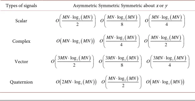
asymmetric.

The symmetry is of great importance to greatly decreasing the calculation complexity of them. Table 1 lists the calculation complexity of different types of signals. It gives the conclusion that the symmetry can decrease the calculation complexity by a few times. Meanwhile, the calculation complexity will increase with the number of components by a few times.

Meanwhile, the calculation complexity of QLCT for different signals is mul-tiplications. Also, the complexity of QCV and QCR for the same type of signals is the same and is much less than calculation in time-domain directly.

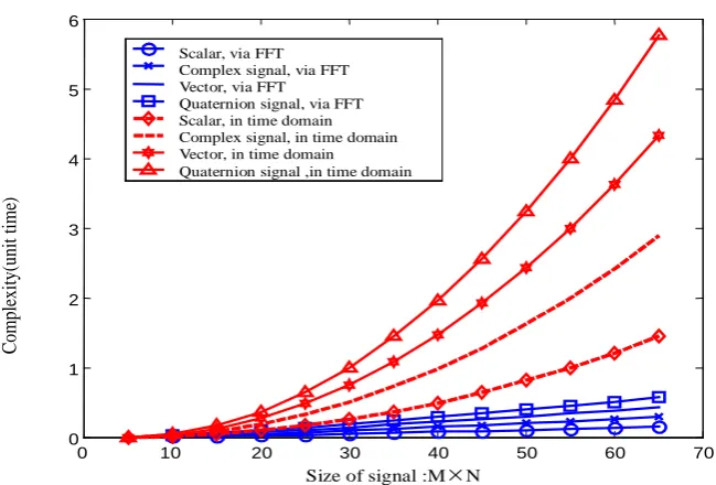
Figure 1 shows one intuitive result. The QCR of the quaternion signal

( )

,

f x y and kernel h x y

( )

, is calculated. We take different signals (scalar,

complex, vector and quaternion) as the convolution kernel h x y

( )

, . The red

[image:12.595.209.534.571.739.2]

lines denote the complexity of implementing QCR in time domain directly, and the blue lines denote the complexity of implementing QCR via FFT. For example,

Table 1. The calculation complexity of QLCT for different signals.

Types of signals Asymmetric Symmetric Symmetric about x or y

Scalar log2( )

2

MN MN

O ⋅ 

 

( ) 2 log

8

MN MN

O ⋅ 

 

( )

2 log

4

MN MN

O ⋅ 

 

Complex O MN

(

⋅log2(MN)

)

( )

2

log 4

MN MN

O ⋅ 

 

( )

2

log 2

MN MN

O ⋅ 

 

Vector 3 log2( )

2

MN MN

O ⋅ 

 

( )

2

3 log

8

MN MN

O ⋅ 

 

( )

2

3 log

4

MN MN

O ⋅ 

 

Quaternion O

(

2MN⋅log2(MN)

)

( ) 2

log 2

MN MN

O ⋅ 

(13)

[image:13.595.211.536.67.287.2]

Figure 1. The comparison of complexity via FFT and calculation directly.

when the size is 60, there is one nearly-ten-times relationship. Moreover, with the increase of size the gap would become bigger and bigger.

6. Conclusion

One contribution of this paper is that the definition of QLCT is obtained, and its properties are given, and its generalization is proved. The reversibility property disclosed the efficiency of QLCT. The linear property indicated that LCT is li-near transform. Another contribution of this paper is that the QCV and QCR of LCT are defined and their relationships and physical interpretation are discov-ered: the fractional convolution of two quaternion signals is to the summation of product of their components, conjugated or odd-even operated, and the product is frequency modulated by chirps; and the product, frequency modulated by a chirp, of two quaternion signals is to the summation, amplitude modulated, of their pseudo convolution; and the correlation of two quaternion signals is to the summation of convolution of their components, which are conjugated or odd-even operated. The last contribution is that the complexity of QLCT, QCV and QCR are given, and its Fast Algorithm is obtained through implementing them via the product theorem in transformed domain whose complexity is simi-lar to FFT, which is of great importance to engineering use [31] [32].

Acknowledgements

This work was fully supported by the NSFCs (61471412, 61771020, 61002052, 61250006).

Conflicts of Interest

The authors declare no conflicts of interest regarding the publication of this pa-per.

0 10 20 30 40 50 60 70

0 1 2 3 4 5 6

Scalar, via FFT Complex signal, via FFT Vector, via FFT

Quaternion signal, via FFT Scalar, in time domain Complex signal, in time domain Vector, in time domain

Quaternion signal ,in time domain

Size of signal :M×N

C

omp

le

xity

(u

nit time

(14)

References

[1] Exampleh, V., Ozaktas, M. and Aytur, O. (1995) Fractional Fourier Domains. Signal Process, 46, 119-124.https://doi.org/10.1016/0165-1684(95)00076-P

[2] Tao, R., Deng, B. and Wang, Y. (2009) Theory and Application of the Fractional

Fourier Transform. Tsinghua University Press, Beijing.

[3] Moshinsky, M. and Quesne, C. (1971) Linear Canonical Transformations and Their Unitary Representation. Journal of Mathematical Physics, 12, 1772-1783.

https://doi.org/10.1063/1.1665805

[4] Xu, G.L., Wang, X.T. and Xu, X.G. (2009) The Logarithmic, Heisenberg’s and Windowed Uncertainty Principles in Fractional Fourier Transform Domains. Signal Processing, 89, 339-343.https://doi.org/10.1016/j.sigpro.2008.09.002

[5] Xu, G.L., Wang, X.T. and Xu, X.G. (2009) Generalized Hilbert Transform and Its Properties in 2D LCT. Signal Process, 89, 1395-1402.

https://doi.org/10.1016/j.sigpro.2009.01.009

[6] Mendlovic, D. and Ozaktas, H.M. (1993) Fractional Fourier Transforms and Their Optical Implementation: I. Journal of the Optical Society of America A, 10, 1875-1881.

[7] Ozaktas, H.M. and Mendlovic, D. (1993) Fractional Fourier Transforms and Their Optical Implementation. II. Journal of the Optical Society of America A, 10, 2522-2531.https://doi.org/10.1364/JOSAA.10.002522

[8] Pei, S.C. and Yeh, M.H. (1998) Two Dimensional Discrete Fractional Fourier Transform. Signal Processing, 67, 99-108.

https://doi.org/10.1016/S0165-1684(98)00024-3

[9] Aytur, O. and Ozaktas, H.M. (1995) Non-Orthogonal Domains in Phase Space of

Quantum Optics and Their Relation to Fractional Fourier Transforms. Optics Communications,120, 166-170.https://doi.org/10.1016/0030-4018(95)00452-E

[10] Ozaktas, H.M., Zalevsky, Z. and Kutay, M.A. (2000) The Fractional Fourier Trans-form with Applications in Optics and Signal Processing. Wiley, New York.

[11] Hamilton, W.R. (1864) Elements of Quaternions. Longman, London.

[12] Xu, G.L., Wang, X.T. and Xu, X.G. (2010) On Uncertainty Principle for the Linear Canonical Transform of Complex Signals. IEEE Transactions on Signal Processing, 58, 4916-4918.https://doi.org/10.1109/TSP.2010.2050201

[13] Stark, H. (1971) An Extension of the Hilbert Transform Product Theorem. Pro-ceedings of the IEEE, 59, 1359-1360.

[14] Havlicek, J.P., Havlicek, J.W., Ngao, D., et al. (1998) Skewed 2D Hilbert Transforms and Computed AM-FM Models. Proceedings 1998 International Conference on Image Processing, Chicago, 7 October 1998, 602-606.

[15] Xu, G.L., Wang, X.T. and Xu, X.G. (2008) Extended Hilbert Transform for Multi-dimensional Signals.2008 5th International Conference on Visual Information En-gineering, Xi’an, 29 July-1 August 2008, 292-297.

[16] Hahn, S.L. (1992) Multidimensional Complex Signals with Single-Orthant Spectra.

Proceedings of the IEEE, 80, 1287-1300.

[17] Moxey, C.E., Sangwine, S.J. and Ell, T.A. (2003) Hypercomplex Correlation Tech-niques for Vector Images. IEEE Transactions on Signal Processing, 51, 1941-1953. https://doi.org/10.1109/TSP.2003.812734

[18] Xu, G.L., Wang, X.T. and Xu, X.G. (2007) Neighborhood Limited Empirical Mode

(15)

on Image and Graphics, Sichuan, 22-24 August 2007, 149-154.

[19] Xu, G.L., Wang, X.T. and Xu, X.G. (2008) Fractional Quaternion Fourier Trans-form, Convolution and Correlation. Signal Processing, 88, 2511-2517.

https://doi.org/10.1016/j.sigpro.2008.04.012

[20] Sangwine, S.J. and Ell, T.A. (1999) Hypercomplex Auto- and Cross-Correlation of

Color Images. Proceedings of the 1999 International Conference on Image

Processing, Kobe, 24-28 October 1999, 319-322.

[21] Ell, T.A. (1993) Quaternion-Fourier Transforms for Analysis of Two-Dimensional Linear Time-Invariant Partial Differential Systems. Proceedings of 32nd IEEE Con-ference on Decision and Control, San Antonio, 15-17 December 1993, 1830-1841. https://doi.org/10.1109/CDC.1993.325510

[22] Xu, G.L., Wang, X.T. and Xu, X.G. (2009) Improved Bi-Dimensional EMD and Hilbert Spectrum for the Analysis of Textures. Pattern Recognition, 42, 718-734. https://doi.org/10.1016/j.patcog.2008.09.017

[23] Ell, T.A. (1992) Hypercomplex Spectral Transforms. Ph.D. Dissertation, University of Minnesota, Minneapolis.

[24] Pei, S.C., Ding, J.J. and Chang, J.H. (2001) Efficient Implementation of Quaternion

Fourier Transform, Convolution, and Correlation by 2-D Complex FFT. IEEE

Transactions on Signal Processing, 49, 2783-2797. https://doi.org/10.1109/78.960426

[25] Duhamel, P. (1986) Implementation of Split-Radix FFT Algorithms for Complex,

Real and Real-Symmetric Data. IEEE Transactions on Acoustics, Speech, and Signal Processing, 34, 285-295.https://doi.org/10.1109/TASSP.1986.1164811

[26] Almeida, L.B. (1997) Product and Convolution Theorems for the Fractional Fourier Transform. IEEE Signal Processing Letters, 4, 15-17.

https://doi.org/10.1109/97.551689

[27] Zayed, A.I. (1998) A Convolution and Product Theorem for the Fractional Fourier Transform. IEEE Signal Processing Letters, 5, 101-103.

https://doi.org/10.1109/97.664179

[28] Akay, O. and Boudreaus, G.F. (1998) Linear Fractionally Invariant Systems: Frac-tional Filtering and Correlation via FracFrac-tional Operators. Conference Record of the

31st Asilomar Conference on Signals, Systems and Computers, Vol. 2, Pacific Grove, 2-5 November 1997, 1494-1498.

[29] Deng, B., Tao, R. and Wang, Y. (2006) Convolution Theorems for the Linear

Ca-nonical Transform and Their Applications. Science in China F, 49, 592-603. https://doi.org/10.1007/s11432-006-2016-4

[30] Xu, G., Wang, X. and Xu, X. (2012) On Analysis of Bi-Dimensional Component Decomposition via BEMD. Pattern Recognition, 45, 1617-1625.

https://doi.org/10.1016/j.patcog.2011.11.004

[31] Xu, G., Zhou, L., Wang, X. and Xu, X. (2017) Assisted Signals Based Mode Decom-position. International Conference on Image, Vision and Computing, Chengdu, 2-4 June 2017, 868-874.

[32] Xu, G., Wang, X., Zhou, L. and Xu, X. (2018) Image Decomposition and Texture

Analysis via Combined Bi-Dimensional Bedrosian’s Principles. IET Image