Incomplete Price Adjustment and Inflation Persistence

Munich Personal RePEc Archive

Incomplete Price Adjustment and

Inflation Persistence

Marcelle, Chauvet and Insu, Kim

University of California Riverside, Jeonbuk National University

4 December 2019

Incomplete Price Adjustment and Inflation Persistence

Marcelle Chauvet

and Insu Kim

December 4, 2019

Abstract

This paper proposes a sticky inflation model in which inflation persistence is endogenously generated from the optimizing behavior of forward-looking firms. Although firms change prices periodically, their ability to fully adjust them in response to changes in economic conditions is assumed to be constrained due to the presence of managerial and customer costs of price adjustment. In essence, the model assumes that price stickiness arises from a combination of staggered contracts as in Calvo (1983) as well as quadratic adjustment cost as in Rotemberg (1982). We estimate the model using Bayesian techniques. Our findings strongly support both sources of price stickiness in the U.S. data. The model performs well in matching microeconomic evidence on price setting, particularly regarding the size and frequency of price changes. The paper also shows how incomplete price adjustments in a staggered price contracts model limit the contribution of expectations to inflation dynamics: it generates the delayed response of inflation to demand and monetary shocks, and the observed correlation between inflation and economic activity.

Keywords: Inflation Persistence, Phillips Curve, Sticky Prices, Convex Costs, Incomplete Price Adjustment, Infrequent Price Adjustment.

JEL Classification: E31

∗_{Department of Economics, University of California, Riverside, CA 92507 (email: chauvet@ucr.edu)}

†_{Corresponding author: Department of Economics, Jeonbuk National University, Seoul, Korea (email: insu.kim@jbnu.ac.kr). An early draft}

of this paper was circulated under the title “Microfoundations of Inflation Persistence in the New Keynesian Phillips Curve.” We would like to thank Martin Eichenbaum, Guillermo Calvo, Mark Watson, Tao Zha, Carlos Carvalho, and participants at seminars given at Oberlin College, the Federal Reserve Bank of Cleveland, Bank of Korea, and at the 17th Meeting of the Society for Nonlinear Dynamics and Econometrics, the 2014 Midwest Macro Meeting, the 2014 North American Summer Meeting of the Econometric Society, the 3rd Vale/EPGE Conference "Business Cycles," the UCR Conference "Business Cycles: Theoretical and Empirical Advances," and the 2019 Conference of the International Association for Applied Econometrics for helpful comments and suggestions. This work was supported by research funds for newly appointed professors of Jeonbuk National University in 2017.

1

Introduction

The standard New Keynesian Phillips curve (NKPC) based on the optimizing behavior of price setters in the presence of nominal rigidities is mostly built on the models of staggered contracts of Taylor (1979, 1980) and Calvo (1983), as well as the quadratic adjustment cost model of Rotemberg (1982). This framework is broadly used in the analysis of monetary policy. Price rigidity works as the main transmission mechanism through which monetary policy impacts the economy.

Although the NKPC has some theoretical appeal, there is growing concern on its empirical shortcom-ings regarding the ability to match some stylized facts on inflation dynamics and the effects of monetary policy. In particular, the standard NKPC models have been criticized due to the failure to generate inflation persistence.1 _{Accordingly, although the price level responds sluggishly to shocks, the inflation}

rate does not. In addition, these models do not yield the result that monetary policy shocks cause a delayed and gradual effect on inflation. Fuhrer and Moore (1995) and Nelson (1998), among others, point out that in order for a model to fully explain the time series properties of aggregate inflation and output gap, it requires not only the price level but also the inflation rate be sticky.

In response to those critiques, this paper proposes a sticky inflation model that is able to endogenously generate inflation persistence as a result of the optimizing behavior of forward-looking firms. In addition, the model implies that monetary policy shocks first impact economic activity, and subsequently inflation but with a long delay, reflecting inflation inertia. The model is also able to capture the observed joint dynamic correlation between inflation and output gap.

We consider that firms face two sources of price rigidities that are related to both the inability to change prices frequently and the cost of sizable adjustments. Calvo’s (1983) staggered price setting has been the most frequently used framework in the literature to derive the NKPC, with a fraction of firms completely adjusting their prices to the optimal level at discrete time intervals. Another popular framework is Rotemberg (1982) in which firms set prices to minimize deviations from the optimal price subject to quadratic frictions of price adjustment. While both the Calvo pricing and the quadratic cost of price adjustment are designed to model sticky prices, the former is related to the frequency of price changes while the latter is associated with the size of price changes. In addition, these models have different implication for the frequency of price changes: Rotemberg’s model yields continuous price adjustment while Calvo’s model implies staggered price setting.

Costs of price adjustment might arise from managerial costs (information gathering and decision making) and customer costs (negotiation, communication, fear of upsetting customers, etc.). For ex-ample, Zbaracki, and Ritson, Levy, Dutta, and Bergen (2004), using data from a large U.S. industrial manufacturer, document evidence that those costs of price adjustment are sizable and convex. However, in contrast to the implication of the Rotemberg pricing, the company that faces convex costs of price adjustment does not change prices continuously but only annually because “it is not the culture” of that industry to have frequent price changes. The culture instead implies that prices are fixed by implicit contracts for several periods. This is also found in a survey of around 11,000 firms in the Euro area by

1

Fabiani et al. (2005), in which implicit and explicit contracts theories were ranked, respectively, first and second among the explanations for price stickiness.

This article proposes a model that combines staggered price setting and quadratic costs of price adjustment in a unified framework. Firms face two decision problems: when to change prices - associated with the Calvo pricing, and how much to change prices - related to quadratic costs of price adjustment. Firms face quadratic adjustment costs only when they decide to change prices, which rather than fixed, varies with the magnitude of the change. The solution of the model implies that, first, prices are not continuously adjusted and, second, firms that are able to change prices do not fully adjust them due to the presence of convex adjustment costs. Inflation persistence is endogenously generated as a consequence of this incomplete and infrequent price adjustment.

Several authors have proposed alternative price settings that can account for some of the empirical facts on inflation and output. The most popular ones are extensions of Calvo’s staggered prices based on backward indexation rules, and staggered price contracts resulting from infrequent information up-dating. These models assume that a fraction of the firms could set their prices optimally each period while the rest adjusts prices according to past aggregate inflation (hybrid NKPC models) or based on outdated information (sticky information models). Although these models are able to generate inflation persistence, either they also imply that firms adjust prices continuously and/or that a fraction of the firms is backward-looking.2 _{The empirical implication that prices change frequently in these models}

contradicts widespread micro-data studies. A recent extensive literature on micro-data shows pervasive evidence of infrequent price adjustments. The finding across countries and different data sources is that firms keep prices unchanged for several months.3

Our model differs from the Calvo-cum-indexation models in which inflation inertia arises from firms’ backward-looking behavior. In our model, inflation persistence is endogenously generated instead from forward-looking firms with optimizing behavior regarding both the size and frequency of price adjust-ments. The combination of incomplete and infrequent price adjustment generates inflation persistence without introducing backward-looking firms. Further, in contrast to the indexation models and sticky information models, prices are not continuously adjusted in the proposed model.4 _{The new Phillips}

curve based on dual stickiness nests the standard NKPC as a special case (Calvo pricing) and offers an alternative to the sticky information Phillips curve and the ad-hoc hybrid NKPC with backward-looking firms.

2

See, e.g., Mankiw and Reis (2002), Christiano, Eichenbaum, and Evans (CEE 2005), and Smets and Wouters (2003, 2007). Notice that continuously price updating is an implication of many other New Keynesian models including Rotemberg (1982) or Kozicki and Tinsley (2002), among several others.

3

See, e.g. Klenow and Kryvtsov (2008), Alvarez, Dhyne, Hoeberichts, Kwapil, Le Bihan, Lunnemann, Martins, Sabbatini, Stahl, Vermeulen, and Vilmunen (2006), Alvarez (2008), Klenow and Malin (2010), Eichenbaum, Jaimovich, and Rebelo (2011), etc. In addition, Blinder, Canetti, Lebow, and Rudd (1998) and Zbaracki, Ritson, Levy, Dutta, and Bergen (2004) provide micro-evidence for variable costs, including managerial and customer costs. International evidence is shown in Angeloni et al. (2006), Alvarez (2008), Nakamura and Steinsson 2008), Bils, Klenow, and Malin 2012, Klenow and Malin 2010, among several others.

4

In this respect, our model is appropriately designed for policy analysis since all firms are forward-looking with optimizing behavior, and

the implied price dynamics match closely the data, as discussed in detail in Section 4.

Additionally, our sticky price model has different implications on price dispersion from the indexation models. While the indexation models imply that price dispersion varies with a change in the inflation rate due to the counterfactual assumption of continuous price adjustments (Giannoni and Woodford 2002), the proposed model implies that price dispersion increases with the magnitude of the inflation rate. In the indexation models a fraction of prices is adjusted optimally, while the remaining prices are updated by automatic indexation to lagged inflation. Accordingly, price dispersion can be inaccurately measured since the prices that may otherwise remain unchanged are instead assumed to be adjusted according to an indexation rule (Chari, Kehoe, and McGrattan 2009). In contrast, our model, as in the standard Calvo price setting, assumes that price dispersion is measured consistently with microeconomic evidence since some prices are optimally adjusted and others remain unchanged.5

Our dynamic stochastic general equilibrium (DSGE) model is estimated using Bayesian techniques. Empirical results indicate strong evidence of incomplete and infrequent price adjustment based on the parameter estimates, supporting the proposed model. Thus, the model provides a theoretical foundation on inflation inertia. In addition, the estimates closely match extensive micro-data evidence regarding the size of price adjustment. In particular, we find that the model has the ability to generate small and even large price changes observed from micro-data. The reason is that the introduction of incomplete price adjustment in a staggered price contracts model leads to an amplification of the impact of cost-push shocks on inflation (large price changes) and a reduction of the response of inflation to demand and monetary shocks (small price changes).6

Our results also show that our model produces relatively more frequent small price changes than models based on the standard NKPC with Calvo pricing, consistently with microeconomic evidence. Klenow and Kryvtsov (2008) document that the Calvo model fails to generate as many small price changes as observed in the micro-data collected for the Consumer Price Index (CPI). On the other hand, our simulation exercise shows that extensions of the Calvo pricing model such as the hybrid NKPC of Smets and Wouters (2007) and models based on the quadratic adjustment cost of Rotemberg (1982) generate too many small price adjustments due to the assumption of continuous price adjustments.

Another result is that the new sticky inflation model implies a delayed and gradual response of inflation to a monetary policy shock, which is in accord with the persistence in inflation observed in

5

The intuition behind this implication is as follows. Suppose that there are only two goods, A and B, in the economy. The price of good A rises, while the price of the other is fixed in a given period. In this case, the aggregate inflation rate rises due to good A, and price dispersion measured by the difference of the goods prices will vary with the size of inflation. The larger the price adjustment, the larger the inflation rate and price dispersion (as well as the welfare loss, Woodford 2003). In contrast to the actual price dispersion, the indexation models assumption of continuous price adjustment counterfactually predicts that the price of B changes with the previous level of inflation. Accordingly, price dispersion varies with the difference between inflation and its lagged value, instead of with the level of inflation (see Giannoni and Woodford, 2002, for detailed explanations). Due to this counterfactual assumption, the indexation models can lead to misleading results when it is used for policy analysis (Chari, Kehoe, and McGrattan 2009), as they inaccurately describe the path of actual price and, therefore, price dispersion.

6

Our model differs from the standard NKPC with Calvo pricing in that the latter implies that firms make relatively large price adjustments

in response to demand and monetary shocks and small price adjustments in response to cost shocks. On the other hand, the hybrid NKPC

models are similar to ours with regard to the muteness of the impact of monetary shock on inflation, which is caused by inflation persistence.

Despite this similarity, the hybrid NKPC does not produce large price changes due to continuous price adjustment, while our model does a

the data. The baseline NKPC with Calvo pricing fails to generate a hump-shaped response of inflation to a monetary policy shock, as inflation falls instantly in response to this shock, displaying no inertia (Christiano, Eichenbaum, and Evans 2005). By contrast, in the proposed model the policy shock raises interest rate and, thus, has a negative impact on output gap and inflation, generating a delayed response of inflation due to the incomplete and infrequent price adjustments.

Regarding the relationship between inflation and output gap, the standard NKPC with Calvo pricing fails to generate the observed low contemporaneous correlation between current output gap and inflation. Our simulation exercise shows that the assumption that firms are able to adjust prices completely in response to changes in economic conditions leads to an unrealistically high correlation between the two variables. The introduction of incomplete price adjustment into a staggered price contracts setting works to reduce the impact of demand-side shocks on prices, leading to a reduction in the estimated positive correlation between inflation and output gap.

The remainder of this paper is organized as follows. Section 2 derives the new sticky inflation model. Section 3 introduces the associated small-scale dynamic stochastic general equilibrium model. Section 4 reports empirical and simulation results, and Section 5 concludes.

2

Firms’ Problems and the Phillips Curve

We assume that the economy has two types of firms: a representative final goods-producing firm and a continuum of intermediate goods-producing firms.

2.1

The Final Goods-Producing Firm

The final goods-producing firm purchases a continuum of intermediate goods, Yit, at input prices,

Pit, indexed byi∈[0,1]. The final good,Yt, is produced by bundling the intermediate goods as follows

Yt=

Z 1

0 Y 1/λf

i,t di

λf

(1)

where 1 ≤ λf < ∞. The final goods-producing firm chooses Yi,t to maximize its profit in a perfectly

competitive market taking both input, Pi,t, and output prices, Pt, as given. The objective of the final

goods-producing firm is expressed as

PtYt−

Z 1

0 Pi,tYi,tdi (2)

subject to the technology described in (1). The first order condition of the final-goods-producing firm implies that

Yi,t =

P

i,t

Pt

−a

Yt (3)

where a ≡ λf/(λf −1) measures the constant price elasticity of demand for each intermediate good.

The relationship between the prices of the final and intermediate goods can be obtained by integrating (3),

Pt=

Z 1

0 P

1/(1−λf)

i,t di

1−λf

. (4)

Equation (4) is derived from the fact that the final goods-producing firm earns zero profits. The final good price can be interpreted as the aggregate price index.

2.2

The Intermediate Goods-Producing Firm

As seen in the literature, the NKPC is most commonly derived using Calvo’s (1983) staggered price setting in which a fraction (1− θ) of firms reset prices to optimize profit while the remaining firms maintain their prices unchanged in any given period. In the Calvo economy, as implied by equation (4), the aggregate price level evolves according to

P

1 1−λf

t = (1−θ) ˜P

1 1−λf

t +θP

1 1−λf

t−1 (5)

where ˜Ptdenotes the aggregate optimal price set by the intermediate good-producing firms. The average

duration of price contracts is calculated as 1/(1−θ) in the Calvo economy. Since individual prices are optimized in a staggered manner, the aggregate price level evolves sluggishly, making the aggregate price depend on its own lag.

Another popular way of introducing nominal rigidities is to assume that firms face variable costs when changing their prices. Rotemberg (1982) proposes that firms face quadratic costs of price adjustment. Several dimensions of managerial and customer relations may imply that the costs of price adjustment is proportional to its size. Since these costs increase with the magnitude of price adjustment, firm’s ability to fully adjust prices could be constrained, making the aggregate price sticky with respect to the size of price changes. We assume that each intermediate goods-producing firm faces the quadratic price adjustment cost given by

QAC = c 2

˜

Pi,t

˜

Pi,t−j

−1

!2

Yt (6)

where ˜Pi,t and ˜Pi,t−j denote firm i’s optimal prices in periodt and t−j, respectively. When the firm i

has no price adjustments between these two periods, the price adjustment cost in periodtis determined by the difference between ˜Pi,,t and ˜Pi,t−j . Equation (6) implies that it is costly for current individual

price to deviate from past price level, which makes price sticky. The cost of adjusting prices is zero when there is no change in nominal price. Our setup is slightly different from that of Rotemberg (1982) since we assume that firms cannot adjust prices continuously.

Zbaracki et al. (2004) document quantitative and qualitative evidence that managerial and customer costs of price adjustment are convex using data from a large U.S. industrial manufacturer, as quoted below:

“The managerial costs of price adjustment increase with the size of the adjustment because the decision and internal communication costs are higher for larger price changes. The larger the proposed price change, the more people are involved, the more supporting work is done, and the more time and attention is devoted to the price change decisions. ... Customer costs of price adjustment also increase with the size of the adjustment because larger price changes lead to both higher negotiation costs and higher communication costs. ... Given the convexity of the price adjustment costs, pricing managers often felt it was not worth the fight to make major

Their findings indicate that the managerial costs and the customer costs are, respectively, 6 and 20 times greater than the menu costs. Although the company investigated by Zbaracki et al. (2004) faces convex costs of price adjustment, it does not change prices continuously as implied by Rotemberg’s sticky price model:

“We can’t change prices biannually, it is not the culture here.”- Pricing manager” (Zbaracki et al. 2004 p.

525)

The company’s infrequent price adjustment can be explained by implicit contract theory. Fabiani et al. (2005) surveyed around 11,000 firms in the Euro area and found that implicit and explicit contracts theories ranked first and second among the explanations of price stickiness. In sum, the company investigated by Zbaracki et al. (2004) adjusts its prices annually, but incompletely due to convex costs of price adjustment.

Both the Calvo pricing and the quadratic cost of price adjustment are similar modeling devices in the sense that they lead to sticky prices. However, they yield different implications with respect to the frequency and size of price adjustment. While the Calvo model is associated with the frequency of price changes, the quadratic price adjustment cost is related to the magnitude of price changes. These pricing models are closely associated with the decision problems faced by firms, regarding when and by how much to change prices. The Calvo pricing is designed to capture infrequent price adjustments that arise from implicit and explicit contracts, coordination failure, and fixed costs of changing prices.7

On the other hand, the Rotemberg pricing is closely related to variable costs such as managerial costs (information gathering and decision making costs), customer costs (negotiation and communication costs), and manager’s “fear of antagonizing customers” (Rotemberg 1982, 2005, Zbaracki et al. 2004). It is worth emphasizing that in our framework firms face variable costs of price adjustment only when they decide to change prices. Evidence on these frictions are extensively found in the the literature as in Zbaracki et al. (2004), and in the surveys by Blinder et al. (1998) or Fabiani et al. (2005).

The intermediate goods-producing firm maximizes real profit from selling its output in a monopo-listically competitive goods market, assuming that its price is fixed with the Calvo probabilityθ in any given period. Additionally, the firm faces the quadratic cost of adjusting its price. The firm i chooses

˜

Pi,t to maximize

Et ∞

X

k=0

(θβ)k





˜

Pi,t−exp(eπ,t)mct+kPt+k

Yi,t+k

Pt+k



− c

2 ˜

Pi,t

˜

Pi,t−j

−1

!2

Yt (7)

7

Blinder et al. (1998) document evidence that the theory of coordination failure ranked first in the United States as the main reason for infrequent price changes. As Nakamura and Steinsson (2013) point out, coordination failure in price setting has two essential elements. First, pricing decisions are staggered since firms wait for other firms to change their prices. Second, firms that have an opportunity to adjust prices will adjust them partially in response to various shocks because other firms keep their prices unchanged. In this respect, our model shares these essential elements of the theory of coordination failure even though pricing does not depend on the behavior of other firms. The fundamental difference between these two theories emerges from the ability to generate a lagged inflation term in the Phillips curve. We later show that our model is able to generate small and large price changes while, as Klenow and Willis (2006) point out, a model with strategic complementarities based on Kimball (1995) is hard to reconcile with large price changes.

subject to the demand function described by equation (3). mct represents real marginal cost, and eπ,t

is the cost-push shock. Firm i’s profit depends on ˜Pi,t when it cannot re-optimize its price in period

t+k, with integer k ∈ [0, ∞]. The firm does not face the quadratic adjustment cost in the future as long as the price chosen in period t is not reset. The firm plans to keep the optimal price unchanged with the probability θ in the future. In this respect, this setup differs from that of Rotemberg (1982) that assumes continuous price adjustment. In addition, the firms who reset their prices in period t

are heterogeneous with respect to the time elapsed since their last price adjustments. When the firm i

adjusts its price in period t−j and t, where integer j ∈[1,∞], and keeps the price unchanged between these two periods, the price adjustment cost depends on the distance between ˜Pi,t−j and ˜Pi,,t. Since the

firms resetting prices in periodtdiffer with respect to the time elapsed since their last price adjustment, the aggregate optimal price of the firms resetting prices in period t, ˜Pt, can be written as a weighted

average of their optimal prices, which is given by

˜

P

1 1−λf

t = (1−θ) ˜P

1 1−λf

l1,t + (1−θ)θP˜ 1 1−λf

l2,t + (1−θ)θ

2_P˜

1 1−λf

l3,t +· · ·=

∞

X

j=1

(1−θ)θj−1P˜

1 1−λf

lj,t (8)

where ˜P

1 1−λf lj,t ≡

R

i∈lj,P˜ 1 1−λf

i,t di.8 The set lj includes the firms that adjust prices in period t−j and t and

that keep their prices unchanged between these two periods. The Calvo pricing implies that,among the cohort of the firms who reset their prices in period t, only a fraction (1−θ)θj−1_{of firms adjusts their}

prices in period t−j and keep their prices unchanged until period t−1. When j = 2, the probability that a firm adjusts its price in period t−2 and keep it unchanged until period t−1 is computed to be (1−θ)θ in the Calvo economy.9

Plugging (3) into (7) and then rearranging it in terms of the relative price, ˜pi,t ≡P˜i,t/Pt, yields

Et ∞

X

k=0

(θβ)khp˜i,tX˜t,k−exp(eπ,t)mct+k

(˜pi,tX˜t,k)−aYt+k

i − c 2 ˜ pi,t ˜

pi,t−j

πtπt−1· · ·πt−j+1−1

!2

Yt (9)

where ˜Xt,k ≡1/πt+1πt+2...πt+k when k >0, and ˜Xt,k ≡1 whenk = 0.10 The first order condition of (9)

with respect to ˜pi,t is given by

Et ∞

X

k=0

(θβ)khX˜_t,k−ap˜−_i,ta−1Yt+k

(1−a)˜pi,tX˜t,k+ (a)exp(eπ,t)mct+k

i

=c p˜i,t

˜

pi,t−j

πtπt−1· · ·πt−j+1−1

!

1 ˜

pi,t−j

πtπt−1· · ·πt−j+1Yt. (10)

8

The relationship between the aggregate price level and the aggregate optimal price is described byP

1 1−λf

t = (1−θ) ˜P

1 1−λf

t +θP

1 1−λf

t−1 .

9

When the quadratic cost of price adjustment is assumed to be zero, the model collapses into the standard NKPC in which firms completely adjust their prices, regardless of the history of their price adjustment.

10

Notice that the quadratic adjustment cost can be written as c2

_p˜

i,t

˜ pi,t−j

−1

2

Yt when the cost of adjusting prices is defined as

_P˜_i,t/Pt ˜

Pi,t−j/Pt−j

−1

2

Yt instead of

_P˜_i,t ˜ Pi,t−j

−1

2

Yt. The terms related to current and lagged inflation can be eliminated from the model

Log-linearizing the first order condition yields

Et ∞

X

k=0

(θβ)k[ˆπt+k+ (1−θβ) (eπ,t+k+ ˆmct+k)] = ˆ˜pi,t+ˆπt+

c(1−θβ)

a−1

ˆ˜

pi,t−ˆ˜pi,t−j+ ˆπt+ ˆπt−1+· · ·+ ˆπt−j+1

(11) where ˆ˜p_i,t, Xˆt,k, and ˆmct+k are the log-deviation (denoted by hat) of ˜pi,t, X˜t,k, and mct+k from their

steady state values, respectively. Arranging (11) gives rise to

1 + c(1−θβ)

a−1

!

ˆ˜

p_i,t+ ˆπt+

c(1−θβ)

a−1 (ˆπt+ ˆπt−1· · ·+ ˆπt−j+1) =

c(1−θβ)

a−1 ˆ˜pi,t−j+Et ∞

X

k=0

(θβ)k[ˆπt+k+ (1−θβ) (eπ,t+k+ ˆmct+k)]. (12)

Whenc= 0 as in the standard Calvo model, current real price ˆ˜pi,tis determined by current and expected

values of future inflation and real marginal cost. In contrast to the implication of Calvo model, our model implies that current price is affected by lagged price. Integrating both sides of (11) with respect toi∈lj

yields

Et ∞

X

k=0

(θβ)k[ˆπt+k+ (1−θβ) (eπ,t+k+ ˆmct+k)] = ˆ˜plj,t+ˆπt+

c(1−θβ)

a−1

ˆ˜

plj,t−ˆ˜plj,t−j + ˆπt+ ˆπt−1· · ·+ ˆπt−j+1

(13) where ˆ˜p_lj,t ≡ R

i∈lj,ˆ˜pi,tdi.

11 _{Rearranging (13) delivers the aggregate optimal price of the firms (i ∈ l}

j),

which is given by

ˆ˜

p_lj,t =θβEt pˆ˜lj,t+1+

"

a−1

a−1 +c(1−θβ)

#

ˆ

πt+1

!

+ (1−θβ) (a−1)

a−1 +c(1−θβ)( ˆmct)

+ c(1−θβ)

a−1 +c(1−θβ)



ˆ˜p_l

j,t−j −θβˆ˜plj,t−j+1+

j−1

X

h=0

Et[θβπˆt−h+1−πˆt−h]



+ε_π,t. (14)

The disturbance, επ,t ≡ _a(1₋−₁₊θβ_c)(₍₁a₋−_θβ1)₎eπ,t, to the optimal price is the reparameterized cost-push shock,

which follows an AR(1) process, επ,t = δπεπ,t−1 +νπ,t with νπ,t ∼ N(0, σπ2). Equation (14) shows that

while the contribution of inflation expectations to the optimal price, ˆ˜p_lj,t, increases with the Calvo pricing parameter θ due to ∂

∂θ

_θβ(a−1)

a−1+c(1−θβ)

> 0, it declines with the quadratic price adjustment cost

c due to _∂c∂ _a−θβ₁₊(_ca₍₁−₋1)_θβ) < 0. The coefficient on the lagged price ˆ˜p_lj,t−j increases as the adjustment cost parameter c rises due to ∂

∂c

_c(1−θβ)

a−1+c(1−θβ)

> 0, while it declines as the duration of nominal price contracts rises due to _∂θ∂ _a−1+c(1−_c(1θβ₋)_θβ)<0.The dependence of the optimal price on its own lagged value in our model prevents it from being adjusted drastically, yielding an inertia in inflation dynamics. Since inflation arises due to the firms that reset their prices to optimal levels, the sluggish adjustment of

11

The most recent three price adjustments of each firm in the cohortljoccur at timet,t−j, and at a particular time periodt−j−kwhere

integerk∈[1,2,· · ·,∞]. Notice thatkdiffers across the firms in the cohortlj whilej is the same in the cohortlj . The aggregated optimal

price in the cohortljat timet−jcan be written as ˆ˜plj,t−_j= ˆ˜p_t−_jwhere ˆ˜p_t−_jis the aggregate optimal price for all the firms that adust prices

at timet−j. This equality holds because the firms in the cohortljare randomly chosen among all the firms that adust prices at timet−j.

the optimal price yields inflation persistence. Turning to the coefficient of real marginal cost, we find that both infrequent and incomplete price adjustments reduce the response of the optimal price to real marginal cost due to _∂c∂ _a(1₋−₁₊θβ_c)(₍₁a₋−_θβ1)₎ < 0 and _∂θ∂ _a(1₋−₁₊θβ_c)(₍₁a₋−_θβ1)₎ < 0. In this respect, our model shares some properties of the Calvo model combined with strategic complementarity in which, along with price stickiness, the presence of strategic complementarity in price setting diminishes the response of “reset prices” to real marginal cost.12 _{However, our model differs from sticky price models with strategic}

complementarity, as in the latter the optimal price does not rely on its own lagged value. In our model, the dependence of inflation on its own lag generates a hump shaped response of inflation to a monetary shock. In section 4, we show that our model does a good job in matching the empirical response of inflation to a monetary shock. We also study whether abstracting the term, Pj−1

h=0Et[θβπˆt−h+1−πˆt−h]

from (14) affects the performance of the model with respect to the ability to generate a sluggish response of inflation to a monetary shock.

Log-linearizing (5) and (8) associated with the Calvo pricing delivers the following equations:

ˆ˜

pt=

θ

1−θπˆt (15)

ˆ˜

p_t= (1−θ) ∞

X

j=1

θj−1ˆ˜p_lj,t. (16)

Equation (15) and (16) show that inflation arises due to the firms resetting their prices. In our setup, there is no closed-form solution for the Phillips curve since firms resetting prices differ in terms of the time elapsed after last price adjustment. Inflation dynamics are described by (14), (15), and (16).

The proposed model nests the standard NKPC model with Calvo setting as a particular case. When the quadratic cost of price adjustment is zero, our model collapses into the standard NKPC of the form

ˆ

πt=βEtπˆt+1+

(1−θ)(1−θβ)

θ mcˆ t+ǫπ,t. (17)

Abstracting the quadratic adjustment from the model makes firms choose the same price regardless of when they reset them. As a consequence, the absence of the adjustment cost yields the standard NKPC.

3

A Small Scale DSGE Model

We consider a small scale DSGE model consisting of the IS curve, the Phillips curve, and the Taylor rule, which is standard in the macroeconomics literature except for our proposed firms’ pricing behavior. As in Erceg, Levin, and Henderson (2000), Christiano, Eichenbaum, and Evans (2005), and Smets and Wouters (2007), we assume that each household is a monopolistic supplier of a differentiated labor service. It is assumed that perfect consumption insurance is available to each household and full risk

12

sharing allows each household to enjoy the same level of consumption.13

The intertemporal utility function of the household is given byEtP∞k=0βk

(Ct+k−hCt+k−1)1

−1/σ

1−1/σ − N_i,t+k1+ϕ

1+ϕ

,

subject to the budget constraint, Ct+k+B_Ptt+_+kk = Wi,t+k_Pt+N_ki,t+k +exp(−ξt+k−1)(1 +it+k−1)(Bt+k

−1

Pt+k ) + Πt+k,

where Ct is the composite consumption good, Wi,t is the nominal wage for each labor type, Πt is real

profits received from firms, and Bt is the nominal holdings of one-period bonds that pay a nominal

in-terest rateit. The parameterh captures the degree of habit in consumption. As in Smets and Wouters

(2007), we introduce a risk premium,−ξt−1, into the DSGE model. The model economy results in the

IS curve, which is given by

yt= Γ1yt−1+ Γ2Etyt+1−Γ3Etyt+2−Σ (it−Etπt+1) +εy,t (18)

where Γ1 ≡ _1+hh_+h2_β, Γ2 ≡

1+hβ+h2_β

1+h+h2_β , Γ3 ≡

hβ

1+h+h2_β, and Σ ≡

σ(1−h)(1−hβ)

1+h+h2_β . The term yt and it denote

output gap and the nominal interest rate, respectively14_{. We interpret the disturbance term as a}

prefer-ence shock, εy,t≡ σ(1₁₊−h_h)(1_+h−2_βhβ)ξt, which is assumed to follow an AR(1) process, εy,t=δyεy,t−1+νy,t with

νy,t ∼N(0, σy2).

Following Erceg, Levin, and Henderson (2000), we assume that a fractionθw of households optimally

adjusts their wages and the remaining households keep their wages unchanged in any given period. Then, the wage inflation Phillips curve can be written as

πw_t =βEtπtw+1+κw(mrst−wt) (19)

where κw ≡ (1−_θθ_ww₍₁₊)(1−_bϕβθ₎w) . The parameter b is the elasticity of substitution across differentiated labor

services, πw

t is wage inflation, wt is the real wage rate, and mrst is the marginal rate of substitution

between consumption and labor, which has the form ofmrst =

ϕ+_σ(1−1+_hβh₎₍₁2β_−h)yt−_σ(1−hβh_)(1−h)yt−1−

hβ

σ(1−hβ)(1−h)Etyt+1. Wage inflation evolves according to (19) while inflation dynamics are governed by

(14), (15), and (16), as described previously. The real marginal cost is defined as mct =wt+nt−yt.

We introduce the identity equation that links real wage growth, wage inflation, and price inflation as follows

wt−wt−1 =πtw−πt. (20)

since we hold Wt/Pt

Wt−1/Pt−1 =

Wt

Wt−1

Pt−1

Pt .

The monetary authority adjusts the interest rate in response to expected inflation and output gap through

it=ρit−1+ (1−ρ)(απEtπt+1+αyyt) +εi,t (21)

where the monetary shock εi,t follows an AR(1) process, εi,t =δiεi,t−1 +νi,t with with N(0, σ2i), and ρ

measures the degree of interest rate smoothing in monetary policy. We assume that policy makers are forward-looking in stabilizing inflation. However, they adjust the interest rate in response to current

13

Households are homogeneous with respect to consumption and bond holdings, whereas they are heterogeneous with respect to hours worked and the wage rate they receive from firms.

14

In this section, the variables with lower-case letters denote log-deviations from their steady state values. We present them without hat for convenience.

economic activity. The monetary authority’s responses to inflation and output gap are determined by the parameters απ and αy, respectively.

4

Empirical Results

4.1

Data and Priors

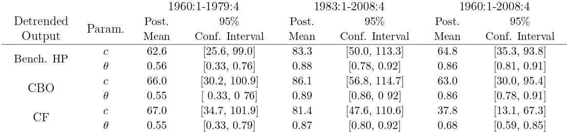
The small scale DSGE model has three observed time series – interest rate, output gap, and inflation; and three shocks – demand, monetary, and cost shocks. In order to estimate the DSGE model, we use real GDP, the effective Federal Funds rate, and the GDP deflator from the FRED database of the Federal Reserve Bank of Saint Louis. Real GDP is detrended using Hodrick–Prescott (HP) two-sided filter. We first focus the analysis on the post-1980 period due the concern that the earlier high inflationary period could be a source of inflation persistence. We also estimate the model for the pre-1980 period and for a larger sample that include the Great Inflation and Great Moderation periods, from 1960 to 2008 (subsection 4.8). Additionally, since interest rate was close to zero between 2009 and 2015, our sample ends in 2008:4 to avoid issues related to the zero lower bound and the unusual dynamics during the recent financial crisis.15

The priors on the model parameters are summarized in Table 1. We set the parameterathat measures the constant price elasticity of demand for each intermediate good to 6, as commonly done in the related literature. This implies a steady state markup of price over marginal cost of twenty percent (see, e.g., Rotemberg and Woodford 1992, and Ireland 2001). The elasticity of substitution across differentiated labor services,b, is set to 6 suggesting that the wage markup at steady state is twenty percent. We also set the discount factorβ to 0.99, as commonly assumed in the literature. The parameter ϕ is set to be 1.5 as in Gourio and Noualz (2006) who estimates this parameter using monthly panel data from the National Longitudinal Survey of Youth (NLSY). The model is estimated using Bayesian techniques. We use 400,000 draws to estimate the DSGE model, but only start calculating posterior features after 30,000 draws. The Metropolis-Hastings algorithm is applied to obtain the maximum likelihood estimates.

Equation (16) shows that the contribution of ˆ˜p_lj,t to the aggregate optimal price ˆ˜p_tconverges to zero as the time elapsed after last price adjustment increases (j → ∞). Therefore, we restrict the max of integer j to 8 when estimating the model. The probability that firms reset prices in period t−j and t, and keep their prices unchanged between these two periods is (1−θ)×(1−θ)θj−1_{. When j = 8 and}

the parameter θ is around 0.75, the probability of resetting prices is very close to zero. Extendingj to 12 or larger does not change our estimation results, while larger j involves considerable computing time

15

cost.16

4.2

Estimation Results

Table 1 reports estimation results of the proposed sticky inflation DSGE model. The posterior mean estimates of monetary policy parameters ρ, απ, and αy are similar to the ones found in the literature.

The parameter measuring the degree of interest rate smoothing is estimated to be 0.76. The estimate of

απ associated with the Fed’s response to inflation expectations is 1.33, whereas the estimated parameter

related to the response of the Fed to output gap is 0.55. The posterior mean of θ, the Calvo measure of degree of nominal rigidity, is estimated to be 0.88 during the Great Moderation period. 17 _{Additionally,}

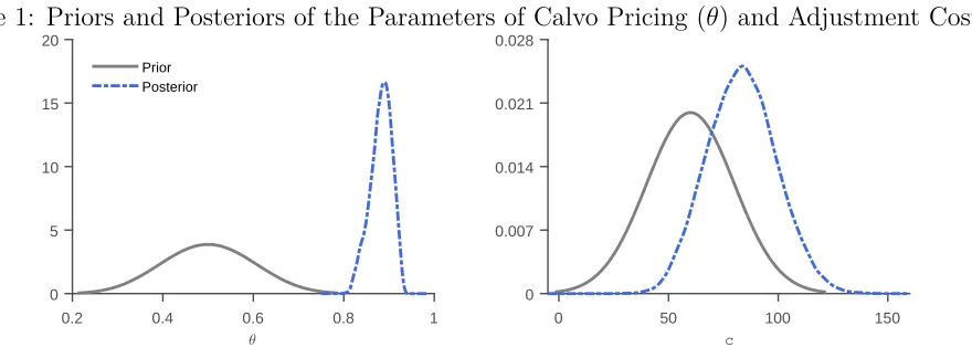
the estimated parameter c associated with variable price adjustment costs is 83.3 and significantly different from zero, even though the Calvo parameter is estimated to be substantially different from zero. This supports evidence that adjustment cost plays an important role in price setting. Figure 1 shows the prior and posterior distributions ofθ and c. The 95% confidence intervals of the parameterθ

and c are substantially away from zero. Thus, the null hypothesis of no price rigidities with respect to the frequency and size of price adjustment is rejected, supporting the proposed sticky inflation model. The parameterθw for staggered wage contracts is estimated to be 0.55, while the estimated parameter σ

determining the sensitivity of output gap to real interest rate is 0.09. The estimated standard deviation of the cost-push shock,σπ, is substantially greater than the standard deviations of the demand shock,σy,

and monetary shock,σi. However, the cost-push shock affects only a small fraction of firms so its impact

on inflation is much smaller than on the optimal price.18

Table 1: Estimation Results - Proposed DSGE Model

Parameter Prior

Distribution

Prior Mean

Prior St. Dev.

Posterior Mean

95%

Confidence Interval

θ Beta 0.5 0.10 0.88 [0.78, 0.92]

c Normal 60.0 20.0 83.3 [50.0, 113.3]

θw Beta 0.5 0.10 0.55 [0.38, 0.72]

σ InvG 0.1 ∞ 0.09 [0.03, 0.19]

ρ Beta 0.7 0.05 0.76 [0.69, 0.84]

απ Normal 1.5 0.25 1.33 [0.89, 1.78]

αy Normal 0.5 0.10 0.55 [0.36, 0.74]

δπ Beta 0.5 0.2 0.50 [0.31, 0.76]

δy Beta 0.5 0.2 0.52 [0.33, 0.69]

δi Beta 0.5 0.2 0.74 [0.60, 0.85]

σπ Invg 0.1 2.0 6.32 [1.37, 9.38]

σy Invg 0.1 2.0 0.07 [0.04, 0.10]

σi Invg 0.1 2.0 0.46 [0.39, 0.51]

16

Settingjbelow or above 12 does not alter our empirical results.

17

As shown in subsection 4.8, the posterior mean of the Calvo parameter changes substantially across samples. For example, our estimates for samples that include high inflation periods are between 0.55 and 0.59, which is consistent with the fact that firms tend to adjust prices more frequently (lowerθ) during high inflationary periods.

18

As an illustration, suppose that the aggregate optimal price rises by 4 percent due to the cost-push shock. In this case, inflation rises by less than 1 percent since the majority of firms keeps their prices unchanged.

Figure 1: Priors and Posteriors of the Parameters of Calvo Pricing (θ) and Adjustment Cost (c)

0.2 0.4 0.6 0.8 1

0 5 10 15 20

Prior Posterior

0 50 100 150

c

0 0.007 0.014 0.021 0.028

4.3

Impulse Response Functions

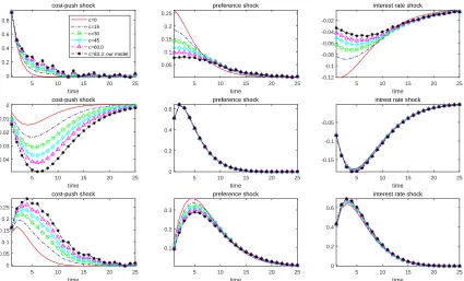
This section shows the impulse response functions (IRFs) for the proposed DSGE model, and the impact of the adjustment costs of prices, c, on the responses. The IRFs are generated using the estimates reported on Table 1, allowing the parameter c to vary from 0, corresponding to the standard NKPC with Calvo pricing, to our proposed DSGE with estimated value of c = 83.3. Figure 2 displays the responses of inflation, output gap, and interest rate to a one-standard deviation cost-push shock (first column), preference shock (second column), and monetary shock (third column).

As shown in the first column, the cost-push shock leads to an immediate increase in inflation re-gardless of the value of c. The response of inflation dies off more gradually as the value of c increases. The monetary authority raises the Federal Funds rate in response to higher inflation, which leads to a decrease in output gap. The shock has the largest impact on output gap after 6 quarters in our model, with the estimate of c is taken into account, while it has the largest effect after 3 quarters for the standard NKPC (c= 0). As shown in Figure 2, higher price adjustment cost implies as a response short-term interest rate that remains high for a considerable time period, yielding a large contraction in economic activity. Accordingly, larger cleads to a more persistent and gradual decline in output gap as a response to cost-push shock. This property of our model is similar to the one of the hybrid NKPC, which also predicts a persistent and positive deviation of inflation from its steady state in the face of the cost-push shock. The similarity is due to the fact that both models consider inflation persistence.

Figure 2: Impulse Response Functions

5 10 15 20 25 time 0 0.2 0.4 0.6 0.8 Inflation cost-push shock c=0 c=15 c=30 c=45 c=60.0 c=83.3: our model

5 10 15 20 25 time 0.05 0.1 0.15 0.2 0.25 preference shock

5 10 15 20 25 time -0.12 -0.1 -0.08 -0.06 -0.04 -0.02

interest rate shock

5 10 15 20 25 time -0.04 -0.03 -0.02 -0.01 0 Output cost-push shock

5 10 15 20 25 time 0 0.2 0.4 0.6 preference shock

5 10 15 20 25 time

-0.15 -0.1 -0.05

intrest rate shock

5 10 15 20 25 time 0 0.05 0.1 0.15 0.2 0.25 Interest Rate cost-push shock

5 10 15 20 25 time

0.1 0.2 0.3

preference shock

5 10 15 20 25 time

0 0.2 0.4 0.6

interest rate shock

Note: _{The estimated IRFs from our proposed DSGE model are the dashed lines with stars corresponding to c= 83.3, while the estimated}

IRFs for the standard NKPC with Calvo pricing are the solid lines with adjustment costc= 0.

However, when firms face large adjustment costs regarding the size of price changes as in our model, the impact of inflation expectations on prices reduces sharply, leading to a gradual rather than an abrupt rise in inflation. The delayed and gradual response of inflation to a change in output gap is an interesting consequence of the proposed model, which considers both infrequent and incomplete price adjustment.

The third column shows the impact of a one-standard deviation monetary policy shock. It is well-known in the literature that the purely forward-looking NKPC with Calvo setting fails to generate a hump-shaped response of inflation to a monetary policy shock. As shown in the figure, the standard NKPC model (c = 0 ) yields an immediate and strong response of inflation to the contractionary monetary shock. By contrast, there is a delayed and gradual response of inflation to the policy shock in our model (c = 83.3), with the largest impact on inflation occurring after 7 quarters. Thus, our proposed model is more in accord with the persistence in inflation.

Figure 3 further compares the impact of a contractionary monetary policy shock in the estimated proposed DSGE model (solid line), with the standard NKPC with Calvo pricing (dash-dotted line), the hybrid NKPC of Smets and Wouters (2007, dashed line), and the VAR(4) model of Christiano, Eichenbaum, and Evans (CEE 1999, solid line with circles). We find that the delayed and hump-shaped response of inflation can be explained by incomplete and infrequent price adjustments in the proposed model, as does the hybrid NKPC model.19 _{On the other hand, the standard NKPC model (c= 0 ) fails}

19

The hybrid NKPC model relies on the ad-hoc indexation assumption to account for inflation persistence, while our theory suggests that inflation persistence can be generated in a forward-looking framework when firms adjust their prices gradually in a staggered price setting.

Figure 3: Impulse Response to a Monetary Policy Shock

0 5 10 15 20 25 30 35 40

time -0.15

-0.1 -0.05 0 0.05 0.1

Inflation

95% CI for VAR(4):CEE(1999) VAR(4):CEE(1999) our model c=0 hybrid model

Note: _{The estimated IRFs from our proposed DSGE model is the solid line with dots corresponding toc= 83.3. The standard NKPC with}

Calvo pricing is the dashed line with adjustment costc = 0. The IRF for the VAR (4) corresponds to the hybrid model from Christiano, Eichenbaum, and Evans (CEE 1999) and is the solid line with dots.

to account for the hump-shaped response of inflation and its impulse response function lies outside of the 95 percent confidence interval of the VAR(4) model. Thus, the standard NKPC is not supported by the empirical VAR model. The figure shows that the VAR(4) model predicts the maximum impact after seven quarters. Our proposed model also predicts the maximum impact of a contractionary monetary policy shock on inflation to be after seven quarters. The hybrid model impulse response displays a shorter impact time, with the maximum occurring after four quarters.

Our model has an amplification effect of cost-push shocks on inflation and a reduced impact of demand and monetary shocks. The predicted lower response of inflation to monetary shock in the hybrid NKPC model is somewhat similar to ours. This similarity is driven by the ability of the hybrid NKPC to generate sluggish movement of inflation in response to shocks. For example, in response to a demand (or expansionary monetary) shock, output positively deviates from its steady state for a considerable time. The standard NKPC with Calvo pricing predicts an immediate rise in inflation since firms are excessively forward-looking. Including a lagged inflation term to the NKPC prevents inflation from jumping from its steady state. Therefore, the response of inflation to the demand-side shocks is reduced.

4.4

Hump-Shaped Response and Alternative Quadratic Cost

This subsection studies whether the hump-shaped response of inflation in the face of a monetary shock is a consequence of the presence of lagged inflation in equation (14). In order to investigate this issue, we

replace the price quadratic cost c

2

˜

Pi,t

˜

Pi,t−j

−1

2

Yt in equation (7), associated with changes in nominal

price, with

_˜

Pi,t/Pt

˜

Pi,t−_j/P_t−_j −1

2

Yt, associated with changes in real price. In this case, equation (9) is

replaced with

Et ∞

X

(θβ)kh(˜pi,tX˜t,k−exp(eπ,t)mct+k)(˜pi,tX˜t,k)−aYt+k

i

− c

2 ˜

pi,t

˜

pi,t−j

−1

!2

This assumption only eliminates the terms associated with current and lagged inflation from the objective function (9) keeping everything else unchanged. With that assumption, the inflation terms are also dropped from the aggregate optimal price of the firms (14), yielding

ˆ˜

p_lj,t =θβEt pˆ˜lj,t+1+

"

a−1

a−1 +c(1−θβ)

#

ˆ

πt+1

!

+ (1−θβ) (a−1)

a−1 +c(1−θβ)( ˆmct)

+ c(1−θβ)

a−1 +c(1−θβ)

ˆ˜

p_lj,t−j−θβˆ˜p_lj,t−j+1+ǫπ,t. (23)

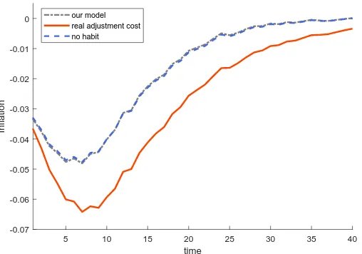
We further investigate whether habit in consumption helps explain the hump-shaped response of infla-tion, by estimating the model for the case when the habit parameter h is zero.

Figure 4: Response of Inflation to Monetary Policy Shock

5 10 15 20 25 30 35 40

time

-0.07 -0.06 -0.05 -0.04 -0.03 -0.02 -0.01 0

Inflation

our model real adjustment cost no habit

Note:_{The estimated IRFs from our proposed DSGE model is the dashed-dotted line. The IRF from our model without habit formation is the}

dashed line, and the IRF from our model with real adjustment cost is the solid line.

Figure 4 displays the response of inflation when a contractionary monetary shock hits the economy. The solid line is associated with the proposed DSGE model with real cost of price adjustment (rather than nominal cost price of adjustment), the dashed line is our DSGE model for the case of h = 0 (no habit), and the dashed-dotted line is our full proposed model with nominal adjustment cost and habit formation. As can be seen, imposingh = 0 does not change the response of inflation at all. In addition, we find that eliminating the terms of lagged inflation from equation (14) by assuming real cost of price adjustment also generates a hump-shaped response of inflation in response to a contractionary monetary shock.20 _{These results show that the hump-shaped response of inflation to monetary shock in our model}

occurs when firms face real or nominal adjustment costs, and when consumers display or not habit persistence, indicating that this result is a consequence of incomplete price adjustment in a staggered price setting.

20

Notice that the fundamental difference between (23) and our proposed NKPC (14) is whether the optimal price depends on lagged inflation.

4.5

Mechanism behind Endogenous Inflation Persistence

We further study how incomplete price adjustment generates inflation persistence endogenously. This is not easy to show given that the assumption of heterogeneous firms with respect to the time elapsed after their last price adjustment implies that it is not possible to derive a closed form solution for inflation dynamics. In order to get an insight on the mechanism endogenously generating inflation persistence, in this subsection we use a simplifying assumption that the firms resetting their prices face the same adjustment cost, c

2

˜

Pt/P˜t−1−1

2

Yt, instead of c₂

˜

Pi,t/P˜i,t−j −1

2

Yt. Our goal is to show

that inflation persistence arises as a consequence of an interaction between infrequent and incomplete price adjustment. In this context, the firm chooses ˜Pt to maximize

Et ∞

X

k=0

(θβ)k

"

( ˜Pt−mct+kPt+k)Yit+k

Pt+k

# − c 2 ˜ Pt ˜

Pt−1 −1

!2

Yt (24)

subject to the demand function described by equation (3). The assumption that the firms resetting prices face the same adjustment cost allows them to choose the same optimal price, delivering a closed-form solution for inflation dynamics. The first order condition is given by

Et ∞

X

k=0

(θβ)khX˜_tk−ap˜−_ta−1Yt+k

(1−a)˜ptX˜tk+ (a)mct+k

i −c " ˜ pt ˜

pt−1

πt−1

#

1 ˜

pt−1

πtYt= 0 (25)

where ˜pt = ˜Pt/Pt. Log-linearization of the first order condition yields

Et ∞

X

k=0

(θβ)kh(ˆ˜pt+ ˆXtk−mcˆ t+k)

i

= c 1−a

ˆ˜

pt−ˆ˜pt−1+ ˆπt

. (26)

Since log-linearization of equation (5) yields ˆ˜p_t = θ

1−θπˆt, the deviation of the optimal price from its

previous one can be written as

ˆ˜

p_t−ˆ˜p_t−1 = [θ/(1−θ)][ˆπt−πˆt−1]. (27)

This equation reveals that the lagged optimal price introduces lagged inflation into the model. Plugging this into equation (26), rearranging the terms, and deleting the hat on the variables for convenience yields

πt = ΛfEtπt+1+ Λlπt−1+λmct (28)

where Λf ≡ η/τ, Λl ≡ κ/τ, λ ≡ ζ/τ, τ ≡ θ(a−1) + c(1−θβ) (1 +θ2β), η ≡ (a−1)θβ +

generate a lagged inflation term as a source of inflation persistence.21

4.6

Dynamic Correlation Between Output Gap and Inflation

Taylor (1999) stresses that the ability to characterize the relationship between output gap and inflation is a criterion for the success of monetary models. This section examines whether the estimated model is able to generate the observed dynamic correlation between inflation and output gap, and the role of incomplete price adjustments in shaping the correlation structure.

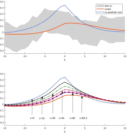
The top panel of Figure 5 displays the dynamic correlation between inflation and output gap gen-erated from our estimated DSGE model and from the standard NKPC with Calvo setting, with the 95 percent confidence interval from the VAR(4) model of Christiano, Eichenbaum, and Evans (CEE 1999). Our proposed model does a reasonable job describing this observed dynamic correlation between inflation and output gap, within the 95 percent empirical confidence interval. On the other hand, the model-implied dynamic correlation changes substantially when the quadratic price adjustment cost is restricted to zero. The standard NKPC model with Calvo pricing does a poor job in predicting the observed dynamic correlation. The contemporaneous correlation between these series implied by the standard NKPC (c= 0) model is abnormally high, in contrast with empirical evidence. This indicates that the assumption of incomplete price adjustments is important in accounting for the output-inflation dynamics.

The bottom panel in Figure 5 show how the overpredicted correlation can be reduced with the quadratic price adjustment cost. We simulate the DSGE model with the parameter c varying from zero as in the standard NKPC model to its estimated value (c = 83.3) in our proposed model, in order to generate the correlation between output gap and inflation. As can be seen, a rise in the price adjustment cost reduces the contemporaneous correlation, leading to a better fit of the data by the model. The intuition behind this result is that the increased cost of price adjustment causes a slower and more gradual response of inflation to demand and monetary shocks, even though the innovations lead to substantial movements in output gap, as shown in Figure 2. Once the three shocks are taken into account simultaneously, the estimated DSGE model predicts the weak, but still positive, contemporaneous correlation between output gap and inflation, due to the reduced response of inflation to the demand-side shocks. When a positive demand shock (or an expansionary monetary shock) hits the economy, forward-looking firms expect that future values of output gap will be positive for a considerable time. Therefore, firms that receive a random signal of price adjustment raise their prices. The impact of this expectation channel on prices is substantial in the standard NKPC with Calvo pricing in which prices are fully adjusted. By contrast, the demand (or monetary) shock has a limited impact on

21

Once the quadratic price adjustment cost is measured with respect to real price as2c

_P˜

t/Pt

˜

Pt−1/Pt−1−1 2

Yt, the first order condition can be

written asEtP

∞

k=0(θβ) k_˜

X−a

tk p˜

−a−1

t Yt+k (1−a)˜ptX˜tk+ (a)mct+k−c

h

˜ pt

˜ pt−1

−1

i

1 ˜ pt−1

Yt= 0. In this case, the resulting Phillips curve

can be written asπt= Λr_fEtπt+1+ Λr_lπt−1+λrmctwhere Λr_f ≡η/τ, Λ_lr ≡κ/τ, λr≡ζr/τr, τr ≡θ(a−1) +c(1−θβ)θ(1 +θβ), ηr≡

(a−1)θβ+c(1−θβ)θ2

β, κr_{≡c(1−θβ)θ, andζ}r_{≡(a−1) (1−θ) (1−θβ). Whenβ= 1,we hold Λ}r

f+ Λrl= 1.

Figure 5: Dynamic Correlation Between Output Gap(t) and Inflation(t+k)

-15 -10 -5 0 5 10 15

k

-0.3 -0.2 -0.1 0 0.1 0.2 0.3 0.4 0.5

95% CI model

no quadratic cost

-15 -10 -5 0 5 10 15

k

-0.3 -0.2 -0.1 0 0.1 0.2 0.3 0.4 0.5

c=0 c=15 c=30 c=45 c=60 c=83.3

Note:_{In the top panel, the solid line is the dynamic correlation from our proposed DSGE model. The dashed line is the standard NKPC with}

Calvo setting (no quadratic cost,c= 0).

prices in our sticky inflation model in which prices adjust slowly.22 _{Our simulation exercise reveals that}

relatively small price changes to demand-side shocks are important features for the success of the model in matching the observed contemporaneous correlation.23 _{This evidence indicates that the assumption}

of incomplete price adjustments is important in accounting for the output-inflation dynamics.

22

Recall that our model implies an amplified response of inflation to supply shocks, as discussed in subsection 4.3.

23

4.7

Size of Price Adjustments

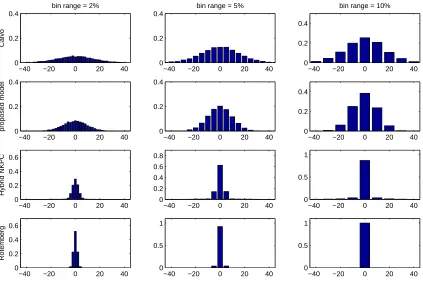
Klenow and Malin (2010) find that price changes are large on average, but also there are many small price changes as well. Alvarez et al. (2016) document evidence on small and large price changes in the U.S. and France Consumer Price Index after correcting for measurement error. This section investigates whether the model of incomplete price adjustment has the ability to generate small and large price changes. We also explore how our model is different from other sticky price models such as the hybrid NKPC of Smets and Wouters (SW 2007), the NKPC with Rotemberg pricing, and the standard NKPC with Calvo pricing. The models are compared with respect to their implied distribution of price changes, i.e., their ability to generate small and large price changes.

Table 2, Figure 6, and Figure 7 display the distribution of price changes of the different models for 1988:1 to 2005:1. This sample period is considered for comparison of our results to Klenow and Kryvtsov (KK 2008) and Nakamura and Steinsson (NS 2008) who use this sample to examine the size of price changes in the U.S. We also show results for the period 1983:1-2008:4 for comparison.24

Figure 6 plots the model-implied distributions of price changes. As can be seen, Rotemberg NKPC model generates more small price changes compared to the other models, with most price changes very close to the mean, and to each other. This is a result of the assumption that firms face adjustment costs that restrict full adjustment to optimal prices. On the other hand, the standard NKPC model with Calvo pricing implies a distribution with the largest variance in price changes. This is because in this model a fraction of firms optimize prices in a staggered manner that can lead to large price changes. Our proposed model and the hybrid NKPC model are in between these two cases. Even though both the hybrid model and our model are designed to generate inflation persistence, there is a fundamental difference between the models with respect to the size of price changes. As shown in the figure, our proposed sticky inflation model produces more small price changes than the standard NKPC with Calvo pricing, and larger price changes than the hybrid NKPC or Rotemberg NKPC models.

Table 2 reports more features of the estimated models’ distribution along with the observed data as found in Klenow and Kryvtsov (KK 2008) and Nakamura and Steinsson (NS 2008). These papers use a large database of the U.S. Consumer Price Index collected by the Bureau of Labor Statistics (BLS), which contains the prices of thousands of individual goods and services. Klenow and Kryvtsov (2008) find that in the U.S. 44% of consumer regular price changes are smaller than 5 percent, 25% are smaller than 2.5 percent, and 12% are smaller than 1 percent, in absolute value. Our proposed model has the closest fit with the observed distribution of price changes. It estimates that 38% of price changes are smaller than 5 percent, 20% are smaller than 2.5%, and 8% are smaller than 1 percent, in absolute value. On one side, Rotemberg NKPC predicts that 100% of prices changes are smaller than 5 percent. On the other, the standard NKPC with Calvo pricing estimates that only 25% of price changes are smaller than 5%. The hybrid NKPC model results are closer to Rotemberg NKPC, predicting that 87% of the

24

Inflation fluctuations were more stable during the period studied by Klenow and Kryvtsov (2008) and Nakamura and Steinsson (2008) (which roughly coincides with Greenspan’s chairmanship at the Federal Reserve) than in the earlier period. We simulate all models with the estimated standard deviations of the shocks matching the observed standard deviation of inflation for the 1988:1-2005:1 period. We additionally report the distribution of price changes but based on theestimated_{standard deviations of the shocks for the 1983:1-2008:4 period}

for comparison.